
Combine text from two or more cells into one cell
You can combine data from multiple cells into a single cell using the Ampersand symbol (&) or the CONCAT function.

Combine data with the Ampersand symbol (&)
-
Select the cell where you want to put the combined data.
-
Type = and select the first cell you want to combine.
-
Type & and use quotation marks with a space enclosed.
-
Select the next cell you want to combine and press enter. An example formula might be =A2&» «&B2.
Combine data using the CONCAT function
-
Select the cell where you want to put the combined data.
-
Type =CONCAT(.
-
Select the cell you want to combine first.
Use commas to separate the cells you are combining and use quotation marks to add spaces, commas, or other text.
-
Close the formula with a parenthesis and press Enter. An example formula might be =CONCAT(A2, » Family»).
Need more help?

See also
TEXTJOIN function
CONCAT function
Merge and unmerge cells
CONCATENATE function
How to avoid broken formulas
Automatically number rows
Need more help?
Want more options?
Explore subscription benefits, browse training courses, learn how to secure your device, and more.
Communities help you ask and answer questions, give feedback, and hear from experts with rich knowledge.
Watch Video – Combine cells in Excel (using Formulas)
A lot of times, we need to work with text data in Excel. It could be Names, Address, Email ids, or other kinds of text strings. Often, there is a need to combine cells in Excel that contain the text data.
Your data could be in adjacent cells (rows/columns), or it could be far off in the same worksheet or even a different worksheet.
How to Combine Cells in Excel
In this tutorial, you’ll learn how to Combine Cells in Excel in different scenarios:
- How to Combine Cells without Space/Separator in Between.
- How to Combine Cells with Space/Separator in Between.
- How to Combine Cells with Line Breaks in Between.
- How to Combine Cells with Text and Numbers.
How to Combine Cells without Space/Separator
This is the easiest and probably the most used way to combine cells in Excel. For example, suppose you have a data set as shown below:
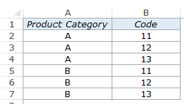
You can easily combine cells in columns A and B to get a string such as A11, A12, and so on..
Here is how you can do this:
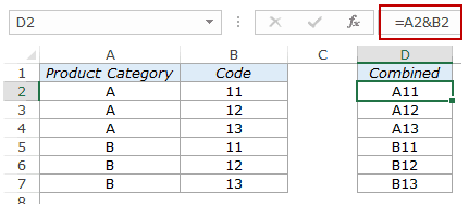
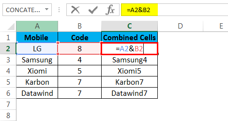
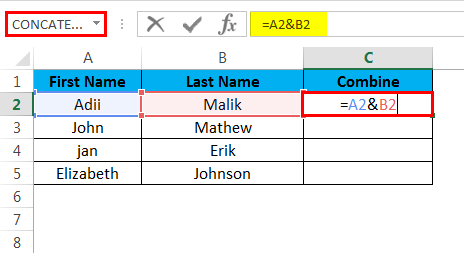
- Enter the following formula in a cell where you want the combined string:
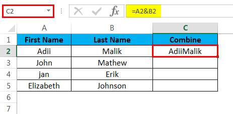
=A2&B2 - Copy-paste this in all the cells.
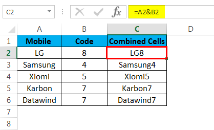
This will give you something as shown below:
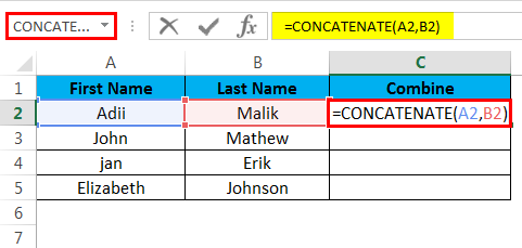
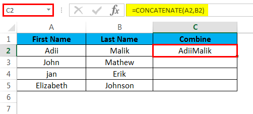
You can also do the same thing using the CONCATENATE function instead of using the ampersand (&). The below formula would give the same result:
=CONCATENATE(A2,B2)
How to Combine Cells with Space/Separator in Between
You can also combine cells and have a specified separator in between. It could be a space character, a comma, or any other separator.
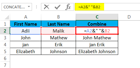
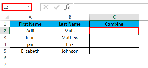
Suppose we have a dataset as shown below:
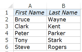
Here are the steps to combine the first and the last name with a space character in between:
- Enter the following formula in a cell:
=A2&" "&B2 - Copy-paste this in all the cells.
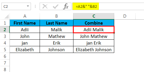
This would combine the first name and last name with a space character in between.

If you want any other separator (such as comma, or dot), you can use that in the formula.
How to Combine Cells with Line Breaks in Between
Apart from separators, you can also add line breaks while you combine cells in Excel.
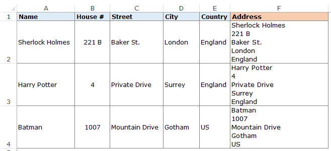
Suppose you have a dataset as shown below:

In the above example, different parts of the address are in different cells (Name, House #, Street, City, and Country).
You can use the CONCATENATE function or the & (ampersand) to combine these cells.
However, just by combining these cells would give you something as shown below:

This is not in a good address format. You can try using the text wrap, but that wouldn’t work either.
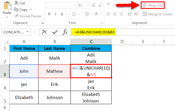
What is needed here is to have each element of the address on a separate line in the same cell. You can achieve that by using the CHAR(10) function along with the & sign.
CHAR(10) is a line feed in Windows, which means that it forces anything after it to go to a new line.
Use the below formula to get each cell’s content on a separate line within the same cell:
=A2&CHAR(10)&B2&CHAR(10)&C2&CHAR(10)&D2&CHAR(10)&E2
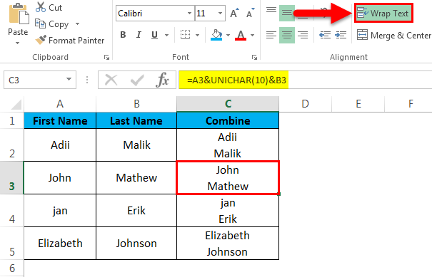
This formula uses the CHAR(10) function in between each cell reference and inserts a line break after each cell. Once you have the result, apply wrap text in the cells that have the results and you’ll get something as shown below:
How to Combine Cells with Text and Numbers
You can also combine cells that contain different types of data. For example, you can combine cells that contain text and numbers.
Let’s have a look at a simple example first.
Suppose you have a dataset as shown below:

The above data set has text data in one cell and a number is another cell. You can easily combine these two by using the below formula:
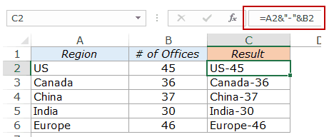
=A2&"-"&B2
Here I have used a dash as the separator.
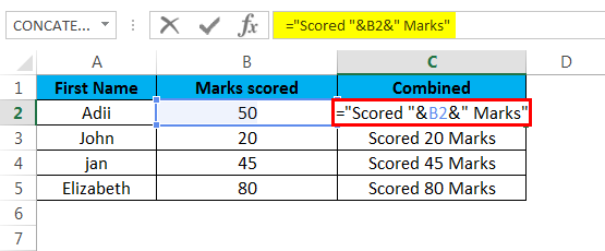
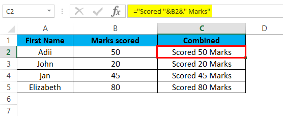
You can also add some text to it. So you can use the following formula to create a sentence:
=A2&" region has "&B2&" offices"
Here we have used a combination of cell reference and text to construct sentences.

Now let’s take this example forward and see what happens when you try and use numbers with some formatting applied to it.
Suppose you have a dataset as shown below, where we have sales values.

Now let’s combine the cells in Column A and B to construct a sentence.
Here the formula I’ll be using:
=A2&" region generated sales of "&B2
Here is how the results look like:

Do you see the problem here? Look closely at the format of the sales value in the result.

You can see that the formatting of the sales value goes away and the result has the plain numeric value. This happens when we combine cells with numbers that have formatting applied to it.
Here is how to fix this. Use the below formula:
=A2&" region generated sales of "&TEXT(B2,"$ ###,0.0")
In the above formula, instead of using B2, we have used the TEXT function. TEXT function makes the number show up in the specified format and as text. In the above case, the format is $ ###,0.0. This format tells Excel to show the number with a dollar sign, a thousand-separator, and one decimal point.
Similarly, you can use the Text function to show in any format allowed in Excel.
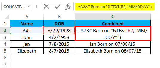
Here is another example. There are names and date of birth, and if you try and combine these cells, you get something as shown below:

You can see that Excel completely screws up the date format. The reason is that date and time are stored as numbers in Excel, and when you combine cells that have numbers, as shown above, it shows the number value but doesn’t use the original format.
Here is the formula that will fix this:
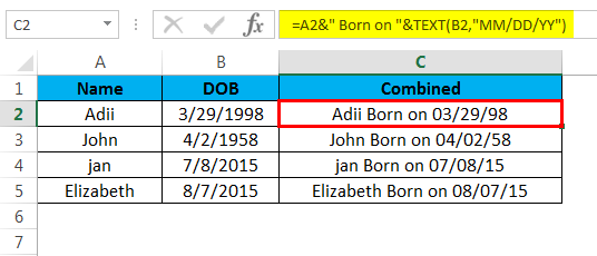
=A2&" was born on "&TEXT(B2,"dd mmm yyy")
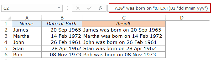
Again, here we have used the TEXT function and specified the format in which we want the Date of Birth to show up in the result.
Here is how this date format works:
- dd – Shows the day number of the date. (try using ddd and see what happens).
- mmm – shows the three-letter code for a month.
- yyy – shows the year number.
Cool… Isn’t it?
Let me know your thoughts in the comments section.
You May Also Like the Following Excel Tutorials:
- CONCATENATE Excel Range (with and without separator).
- How to Merge Cells in Excel the Right Way.
- How to Combine Multiple Workbooks into One Excel Workbook.
- How to Combine Data from Multiple Workbooks into One Excel Table (using Power Query).
- How to Merge Cells in Excel
- How to Combine Duplicate Rows and Sum the Values in Excel
- Combine Date and Time in Excel
Combine cells in Excel (Table of Contents)
- Combine cells in Excel
- Examples of Combine cells in Excel
- How to Use Combine cells in Excel?
Introduction to Combine Cells in Excel
Combine cells in excel is used to combine the 2 or more cell values in a single cell. For this, choose the cells which we need to combine. Go to the cell where we want to see the outcome. Now press the equal sign and select both the cells separated by the ampersand (“&”) sign. For example, if we want to combine cell A1 and A2, then the combine cell formula will look like ”=A1&A2”. We can use any text in the cell quoting it in inverted commas and then selecting a cell separated by an ampersand.
This function is mainly used to combine values from more than one cell to display data in a more useful form, as in the case of the below example.
Concatenate function is different from using the function of the merged cell as the function of the merged cell will combine only cells and not the data of the cells. If we merge cells, then we only physically merge the cells and not the data as in the below case, where only the cells are merged and not the data.

Examples of Combine cells in Excel
Below are the different examples to combine cells in Excel:
You can download this Combine cells Excel Template here – Combine cells Excel Template
- Combine cells in excel without spaces
If we want to combine cells without any spaces, we can simply use “&” to combine cells below.
This is the result of combining cells without any spaces, which is shown below.
- Combine cells in excel with space
We can add space after the content of the first cell by simply adding the space in double Quotes.
This is the result of combined cells with space which are shown below
- Combine cells in excel with a line break
A line break can be added by specifying the character value of a line break that is 10.
This is the result of combined cells with a line break, which are shown below.
- Combine cells in excel with static Text.
This is the result of combined cells with static Text, which is shown below
- Combining date and text
A date cannot be combined with a text in a cell; this can be only done by using the Text function of Excel.
This is the result of combining date and text, which is shown below
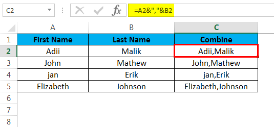
- Combining data with a comma.
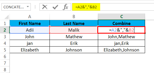
This is the result of combining data with a comma which is shown below
Explanation
When it comes to combining the cells than the concatenate function is the easiest way to combine the data into one cell. This function can save from working overnight by quickly combining the data from the cells.
Concatenate function can be used by the formula or by simply using the “&” sign. The data that can be combined from the cells can be in any form; it may be
- Text
- Date
- Special characters
- Symbols
By using the concatenate function, the data can be easily combined into one cell, as shown in the above examples. The only difference is that the concatenate function comes with a limitation of 255 characters. However, there is no such restriction when it comes to using the symbol “&” for combing the data.
How to Use Combine cells in Excel
Combining cells can be done in any way; this can be done via the formula of concatenating or using the symbol of “&.”
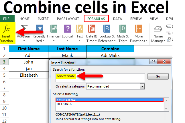
Method 1st by using the function of concatenating.
- Step 1st
First, select the cell where you want the combined data to be displayed.
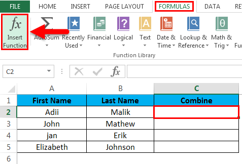
- Step 2nd
Go to the ribbon and select the option of formulas and then select the option of insert function.
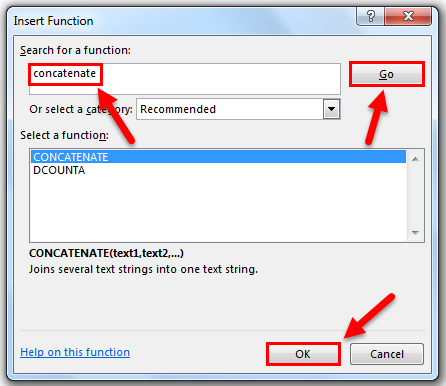
- Step 3rd
Simply type the formula name and click on ok to insert the formula of concatenate.
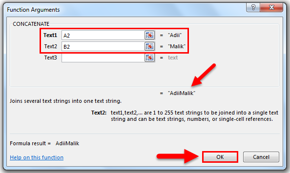
- Step 4th
Give the reference of the cells from where the data is to be combined and click on Ok.
- Step 5th
This is to show how Concatenate function is used in the cell where you want the combined data.
Below is the result of the function and combined data.
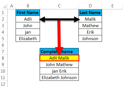
Method 2nd by using the “&”.
“&” can be simply used to combine the data if in case the concatenate function is not used.
- Step 1st
Begin typing with the “=” sign and then select the first part of the text. Now insert “&” and then select the next part of the text and click enter.
- Step 2nd
Below will be the output after enter is pressed.
Things to Remember
- If we are using the concatenate function of Excel, then this is required that there is at least one text argument that is given to the function.
- This should be remembered that Excel has its own limits; this means that a maximum of 255 strings can be combined by using the concatenate function, or they should not be not more than 8,192 in characters.
- Even if we are combing the cells that have numbers, date or any format, the result will always be text.
- Combining cells via concatenating will not work if we are giving array reference to the formula of concatenating. This means that the cells references should be entered individually instead of giving an array to the function.
This means that to combine the cells from A1 to A5; we must write the formulas as
= concatenate (a1, a2, a3,a4,a5) and not as =concatenate(A1: A5)
- If any of the cells that are ought to be combined has an error, then the result will be an error. For example, if cell A1 has an error and we have given reference to this cell in any of the concatenate formula, then the result will be an error. So this is important to note that no cell that is ought to be combined has the error.
- If in case a cell has a date and we want to combine this cell with any other cell, then, in this case, we have to use the “text” function of Excel. A cell that has the date in it cannot be combined by simply using the concatenate; this is because the end result of concatenating is a text.
- Combing the cells via merged cells options will only combine the cells and not the data that is in the cells. This is because the merged cells option only physically combines the cells and is not meant to combine the data of the cells.
- A static text that is to be used while combing the data should be enclosed in Quotation marks; else, the formula will be an error. For example, we must write “= concatenate (“text”, A1)” instead of writing “=concatenate(text, A1).
Recommended Articles
This has been a guide to Combine cells in Excel. Here we discuss the Combine cells in Excel and how to use the Combine cells in Excel along with practical examples and a downloadable excel template. You can also go through our other suggested articles –
- SUM Cells in Excel
- Format Cells in Excel
- How to Add Cells in Excel
- VBA Cells
Combining Excel Cells
Combining cells in excel implies joining the content of two or more cells into a single cell. This allows viewing united values rather than split values. To combine cells, one can use either the ampersand operator (&) or the CONCATENATE function of Excel.
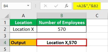
For example, a bank manager wants to view the branch location and the number of employees working there in a single cell. The formula “=A2&”,”&B2” (exclude the beginning and ending double quotation marks) combines cells A2 and B2 containing “location X” and “570” respectively.
Therefore, the output is “location X,570.” The comma of this output serves as a separator (delimiter) between the two cell values. This is shown in the following image.
The purpose of combining excel cells is to arrange the data in the desired format. Moreover, it improves the presentation of data, thereby making the dataset suitable for further processing.
It must be noted that combining excel cells is different from merging cellsMerging a cell in excel refers to combining two or more adjacent cells either vertically, horizontally or both ways. Merging excel cells is specifically required when a heading or title has to be centered over an area of a worksheet.read more. The latter retains the data of the upper-leftmost cell only, while there is no data loss in case of the former. This article discusses the different techniques of combining cells containing diverse data values in Excel.
Table of contents
- Combining Excel Cells
- How to Combine Cells in Excel?
- Example #1–Combine a Text String and Number with the Ampersand Operator
- Example #2–Combine two Text Strings with the Ampersand and CONCATENATE
- Example #3–Combine two Text Strings and add a Line Break with the Ampersand and CHAR
- Example #4–Prefix and Suffix Text Strings to a Number with the Ampersand
- Example #5–Prefix Text Strings to the Current Date with the Ampersand
- Example #6–Combine Cell Values in VBA with the Ampersand
- Frequently Asked Questions
- Recommended Articles
- How to Combine Cells in Excel?
How to Combine Cells in Excel?
Let us consider a few examples to understand the process of combining cells in Excel.
You can download this Combine Cells Excel Template here – Combine Cells Excel Template
Example #1–Combine a Text String and Number with the Ampersand Operator
The succeeding image shows the product name and code in columns A and B respectively. We want to combine the text string (column A) and the numeric value (column B) of each row in a single cell (in column D). Use the ampersand operator.
The steps to combine two excel values using the ampersand operator are listed as follows:
Step 1: Enter the formula “=A4&B4” in cell C4, as shown in the succeeding image.
Note: Notice that in the formula bar of the following image, there is an apostrophe at the beginning of the formula. This apostrophe indicates that this formula is treated as text by Excel. Once the apostrophe is removed, the formula is processed by Excel. Hence, ignore the leading apostrophe of the formula.

Step 2: Press the “Enter” key. The output for the first row is “A8,” as shown in the succeeding image. To obtain the outputs for all the rows, drag the formula to the remaining cells of the column.
For simplicity, we have retained the formulas in column C and given the outputs in column D. Hence, in the first output, the letter “A” and the number 8 have been combined to form “A8.”

Example #2–Combine two Text Strings with the Ampersand and CONCATENATE
The succeeding image shows the first and last names in columns A and B respectively. We want to obtain the full names separated by a space within a single column. Use the ampersand operator and the CONCATENATE function to combine the excel cells of each row.
The steps for combining two cell values using the given techniques are listed as follows:
Step 1: Enter the following formulas in cells C16 and E16 respectively.
- “=A16&” “&B16”
- “=CONCATENATE(A16,” “,B16)”
Step 2: Press the “Enter” key after entering each of the preceding formulas. Next, drag the formula to the remaining cells of the column. The outputs are shown in the succeeding image.
For simplicity, we have retained the formulas using the ampersand and the CONCATENATE in columns C and E respectively. The outputs have been given in columns D and F. Hence, in the first output (D16 and F16), the names “Tanuj” and “Rajput” have been combined to form the full name “Tanuj Rajput.”
Note: In both the formulas, we have enclosed a single space between cells A16 and B16. So, the output also has this space between the first and the last names. However, just to make this space visible, additional spaces have been inserted in the outputs. Ignore these extra spaces and remember that the output will have as many spaces as that of the formula.
Hence, had the formula contained three spaces within the double quotation marks [like “=CONCATENATE(A16,” “,B16)”], the output also would have had three spaces between the first and the last names [like “Tanuj Rajput”].

Example #3–Combine two Text Strings and add a Line Break with the Ampersand and CHAR
The succeeding image shows the first and the last names in columns F and G respectively. We want to combine the two names of each row in a single cell (column I). Further, add a line break between the combined names. Use the ampersand operator and the CHAR function.
The steps to combine the names and insert a line break in excel are listed as follows:
Step 1: Enter the following formula in cell H4.
“=F4&CHAR(10)&G4”
The ampersand combines the first name and the last name. The “CHAR(10)” inserts a line break after the first name and before the last name.
Note 1: “CHAR(10)” returns a line feed, which implies that the data value following it goes to the next line.
Note 2: Ignore the leading apostrophe of the formula, which is displayed in the formula bar. For more details related to this apostrophe, refer to the note (under step 1) of the first example of this article.

Step 2: Press the “Enter” key. Next, select the output cell and click “wrap text”Wrap text in Excel belongs to the “Formatting” class of excel function that does not make any changes to the value of the cell but just change the way a sentence is displayed in the cell. This means that a sentence that is formatted as warp text is always the same as that sentence that is not formatted as a wrap text.read more from the “alignment” group of the Home tab. The final output is shown in cell I4 of the following image.
Hence, in the first output, the names “Tanuj” and “Rajput” have been combined (with a line break in between) to form “Tanuj Rajput.”
To obtain the outputs for the entire column, drag the formula of the preceding step (step 1) to the remaining cells. Next, select the output column and click “wrap text.” For simplicity, we have retained the formulas in column H and given the outputs in column I.
Note: Enabling the “wrap text” option makes the line break of the output visible. If “wrap text” is not applied, the first and the last names are joined together in one line (within a single cell) even though CHAR(10) has been used. Hence, to see the impact of CHAR(10), it is essential to apply “wrap text.”

Example #4–Prefix and Suffix Text Strings to a Number with the Ampersand
The succeeding image shows the number of days in column A. To this number, we want to prefix the string “due in” and suffix the string “days.” Use the ampersand operator.
The steps for the given task are listed as follows:
Step 1: Enter the following formula in cell B34.
=”Due in “&A34&” days”
Note: Notice that the formula contains spaces following the prefix and preceding the suffix. This ensures that spaces are inserted at their respective places in the output.
Step 2: Press the “Enter” key. The output is shown in cell C34 of the succeeding image. Drag the formula entered in the preceding step to the remaining range.
For simplicity, we have retained the formulas in column B and given the outputs in column C.
Hence, the given prefix and suffix have been added to all the numeric values of column A. The outputs of column C represent the terms of a payment schedule.

Example #5–Prefix Text Strings to the Current Date with the Ampersand
We want to prefix the text string “today is” to today’s date. The output should contain the date in the following formats:
- As a serial number of Excel
- As a text string in the format mm-dd-yyyy
For both the preceding pointers, use the ampersand operator and the TODAY function. Use the TEXT function as well for the second pointer.
Note that the date of creation of this article was December 1, 2018. So, all the following calculations take into account the given date.
The steps for the given task are listed as follows:
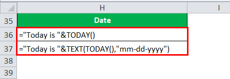
Step 1: Enter the following formulas in cells H36 and H37 respectively.
- “=”Today is “&TODAY()”
- “=”Today is “&TEXT(TODAY(),”mm-dd-yyyy”)”
These formulas are shown in the succeeding image.
Note 1: The TODAY function returns the current date. It updates automatically each time the workbook is opened. It does not take any arguments.
Note 2: The TEXTTEXT function in excel is a string function used to change a given input to the text provided in a specified number format. It is used when we large data sets from multiple users and the formats are different.read more function converts a numeric value to text in the format specified by the user. The syntax is “TEXT(value,format_text).” The “value” is the number to be converted to text. The “format_text” is the format to be applied to the number.
Note 3: Notice that spaces are inserted at the relevant places in both formulas. This inserts spaces in the output.
Step 2: Press the “Enter” key after entering the two preceding formulas. The outputs are displayed in the following image.
Hence, in the first output (cell H36), the TODAY function has returned a serial number (43435). This number corresponds to the date December 1, 2018.
In the second output (cell H37), the date returned by the TODAY function is converted to text (in mm-dd-yyyy format) by the TEXT function. Had we not used the TEXT function, the date would have been displayed as a number.
Therefore, the prefix “today is” has been added to the two date formats with the help of the ampersand operator.

Example #6–Combine Cell Values in VBA with the Ampersand
We want to combine the values of cells A4 and B4 in a single excel cell, C4. Write the VBA code for the same.
The code for combining the cell values (without any data loss) is given as follows:
Sub Mergecells()

  Range(“C4”).Value = Range(“A4”).Value & Range(“B4”).Value

End Sub
Frequently Asked Questions
1. Define the combining of cells in Excel.
The combining of cells is simply the joining of the values of two or more cells. One can use the CONCATENATE function or the ampersand operator (&) to combine cell values. By combining cells, no data is lost, unlike in the case of merging cells.
It is possible to insert a delimiter or a separator (like space, comma, etc.) at the relevant places in the combined output. One can also add a line break for a neat display of the combined output.
Note: For more details on how to combine cell values in Excel, refer to the examples of this article.
2. How to combine two cell values in Excel with a comma, space, semicolon, and hyphen as the delimiters?
The delimiter required in the combined output should be enclosed within double quotation marks in the formula entered initially. To combine values of cells A1 and B1, the Excel formulas containing the given delimiters are stated as follows:
a. Comma: “=CONCATENATE(A1,”,”,B1)” or “=A1&”,”&B1”
b. Space: “=CONCATENATE(A1,” “,B1)” or “=A1&” “&B1”
c. Semicolon: “=CONCATENATE(A1,”;”,B1)” or “=A1&”;”&B1”
d. Hyphen: “=CONCATENATE(A1,”-“,B1)” or “=A1&”-“&B1”
Note 1: A delimiter is a character or symbol that separates two values.
Note 2: While entering the preceding formulas in Excel, ensure that the beginning and ending double quotation marks are excluded.
3. State the Excel formulas (using CONCATENATE and “&”) for combining data in the following cases:
• Three cell values with the space as the delimiter
• Three cell values with the space as the delimiter and a date (in dddd/mm/yyyy format) in the center of the combined output
To combine the values of cells A1, B1, and C1 with spaces in between, use either of the following formulas in Excel:
a. “=CONCATENATE(A1,” “,B1,” “,C1)”
b. “=A1&” “&B1&” “&C1”
To combine the values of cells A1, B1, and C1 where B1 contains a date (12/01/2021) and the space is the delimiter, use either of the following formulas in Excel:
a. “=CONCATENATE(A1,” “,TEXT(B1,”dddd/mm/yyyy”),” “,C1)”
b. “=A1&” “&TEXT(B1,”dddd/mm/yyyy”)&” “&C1”
Note: Exclude the beginning and the ending double quotation marks while entering the preceding formulas in Excel.
Recommended Articles
This has been a guide to combining cells in Excel. Here we discuss how to combine cells in Excel using the ampersand operator (&) and CONCATENATE along with examples and a downloadable template. You may also look at these useful articles of Excel –
- Combine Text From Two Or More Cells into One CellTo combine text from two or more cells into one cell, select the cell to begin with, then type «=» and select the desired cell to combine, then type «&» and use quotation marks with a space enclosed, and finally select the next required cell to connect and press the enter key.read more
- Concatenate Excel ColumnsConcatenating columns in Excel is similar to concatenating data in Excel. Users must give the cell or column reference when concatenating columns, and the result is then displayed in a single cell.read more
- Concatenate Strings in ExcelConcatenation of Strings is accomplished using Excel’s two concatenate methods, the & operator and the concatenate inbuilt function. read more
- Count Colored Cells In ExcelTo count coloured cells in excel, there is no inbuilt function in excel, but there are three different methods to do this task: By using Auto Filter Option, By using VBA Code, By using FIND Method.
read more - Excel TranslateThe Excel Translate function translates any statement or word into another language. It can be found in the language section of the review tab.read more
Merged cells are one of the most popular options used by beginner spreadsheet users.
But they have a lot of drawbacks that make them a not so great option.
In this post, I’ll show you everything you need to know about merged cells including 8 ways to merge cells.
I’ll also tell you why you shouldn’t use them and a better alternative that will produce the same visual result.
What is a Merged Cell
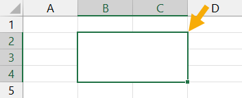
A merged cell in Excel combines two or more cells into one large cell. You can only merge contiguous cells that form a rectangular shape.
The above example shows a single merged cell resulting from merging 6 cells in the range B2:C4.
Why You Might Merge a Cell
Merging cells is a common technique used when a title or label is needed for a group of cells, rows or columns.
When you merge cells, only the value or formula in the top left cell of the range is preserved and displayed in the resulting merged cell. Any other values or formulas are discarded.
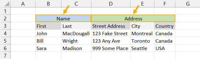
The above example shows two merged cells in B2:C2 and D2:F2 which indicates the category of information in the columns below. For example the First and Last name columns are organized with a Name merged cell.
Why is the Merge Command Disabled?
On occasion, you might find the Merge & Center command in Excel is greyed out and not available to use.
There are two reasons why the Merge & Center command can become unavailable.
- You are trying to merge cells inside an Excel table.
- You are trying to merge cells in a protected sheet.
Cells inside an Excel table can not be merged and there is no solution to enable this.
If most of the other commands in the ribbon are greyed out too, then it’s likely the sheet is protected. In order to access the Merge option, you will need to unprotect the worksheet.
This can be done by going to the Review tab and clicking the Unprotect Sheet command.
If the sheet has been protected with a password, then you will need to enter it in order to unprotect the sheet.
Now you should be able to merge cells inside the sheet.
Merged Cells Only Retain the Top Left Values
Warning before you start merging cells!
If the cells contain data or formulas, then you will lose anything not in the upper left cell.
A warning dialog box will appear telling you Merging cells only keeps the upper-left value and discards other values.
The above example shows the result of merging cells B2:C4 which contains text data. Only the data from cell B2 remains in the resulting merged cells.
If no data is present in the selected cells, then no warning will appear when trying to merge cells.
8 Ways to Merge a Cell
Merging cells is an easy task to perform and there are a variety of places this command can be found.
Merge Cells with the Merge & Center Command in the Home Tab
The easiest way to merge cells is using the command found in the Home tab.
- Select the cells you want to merge together.
- Go to the Home tab.
- Click on the Merge & Center command found in the Alignment section.
Merge Cells with the Alt Hotkey Shortcut
There is an easy way to access the Home tab Merge and Center command using the Alt key.
Press Alt H M C in sequence on your keyboard to use the Merge & Center command.
Merge Cells with the Format Cells Dialog Box
Merging cells is also available from the Format Cells dialog box. This is the menu which contains all formatting options including merging cells.
You can open the Format Cells dialog box a few different ways.
- Go to the Home tab and click on the small launch icon in the lower right corner of the Alignment section.
- Use the Ctrl + 1 keyboard shortcut.
- Right click on the selected cells and choose Format Cells.
Go to the Alignment tab in the Format Cells menu then check the Merge cells option and press the OK button.
Merge Cells with the Quick Access Toolbar
If you use the Merge & Center command a lot, then it might make sense to add it to the Quick Access Toolbar so it’s always readily available to use.
Go to the Home tab and right click on the Merge & Center command then choose Add to Quick Access Toolbar from the options.
This will add the command to your QAT which is always available to use.
A nice bonus that comes with the quick access command is it gets its own hotkey shortcut based on its position in the QAT. When you press the Alt key, Excel will show you what key to press next in order to access the command.
In the above example, the Merge and Center command is the third command in the QAT so the hotkey shortcut is Alt 3.
Merge Cells with Copy and Paste
If you have a merged cell in your sheet already then you can copy and paste it to create more merged cells. This will produce merged cells with the exact same dimensions.
Copy a merged cell using Ctrl + C then paste it into a new location using Ctrl + V. Just make sure the paste area doesn’t overlap an existing merged cell.
Merge Cells with VBA
Sub MergeCells()
    Range("B2:C4").Merge
End Sub
The basic command for merging cells in VBA is quite simple. The above code will merge cells B2:C4.
Merge Cells with Office Scripts
function main(workbook: ExcelScript.Workbook) {
	let selectedSheet = workbook.getActiveWorksheet();
	selectedSheet.getRange("B2:C4").merge(false);
	selectedSheet.getRange("B2:C4").getFormat().setHorizontalAlignment(ExcelScript.HorizontalAlignment.center);
}
The above office script will merge and center the range B2:C4.
Merge Cells inside a PivotTable
We can’t make this change for the selected cells because it will affect a PivotTable. Use the field list to change the report. If you are trying to insert or delete cells, move the PivotTable and try again.
If you try to use the Merge and Center command inside a Pivot Table, you will be greeted with the above error message.
You can’t use the Merge & Center command inside a PivotTable, but there is a way to merge cells in the PivotTable options menu.
In order to avail of this option, you will first need to make sure your Pivot Table is in the tabular display mode.
- Select a cell inside your PivotTable.
- Go to the Design tab.
- Click on Report Layout.
- Choose Show in Tabular Form.
Your pivot table will now be in the tabular form where each field you add to the Rows area will be in its own column with data in a displayed in a single row.
Now you can enable the option to show merge cells inside the pivot table.
- Select a cell inside your PivotTable.
- Go to the PivotTable Analyze tab.
- Click on Options.
This will open up the PivotTable Options menu.
Enable the Merge and center cells with labels setting in the PivotTable Options menu.
- Click on the Layout & Format tab.
- Check the Merge and center cells with labels option.
- Press the OK button.
Now as you expand and collapse fields in your pivot table, fields will merge when they have a common label.
10 Ways to Unmerge a Cell
Unmerging a cell is also quick and easy. Most methods involve the same steps as used to merge the cell, but there are a few extra methods worth knowing.
Unmerge Cells with the Home Tab Command
This is the same process as merging cells from the Home tab command.
- Select the merged cells to unmerge.
- Go to the Home tab.
- Click on the Merge & Center command.
Unmerge Cells with the Format Cells Menu
You can unmerge cells from the Format Cells dialog box as well.
Press Ctrl + 1 to open the Format Cells menu then go to the Alignment tab then uncheck the Merge cells option and press the OK button.
Unmerge Cells with the Alt Hot Key Shortcut
You can use the same Alt hot key combination to unmerge a merged cell. Select the merged cell you want to unmerge then press Alt H M C in sequence to unmerge the cells.
Unmerge Cells with Copy and Paste
You can copy the format from a regular single cell to unmerge merged cells.
Find a single cell and use Ctrl + C to copy it, then select the merged cells and press Ctrl + V to paste the cell.
You can use the Paste Special options to avoid overwriting any data when pasting. Press Ctrl + Alt + V then select the Formats option.
Unmerge Cells with the Quick Access Toolbar
This is a great option if you have already added the Merge & Center command to the quick access toolbar previously.
All you need to do is select the merged cells and click on the command or use the Alt hot key shortcut.
Unmerge Cells with the Clear Formats Command
Merged cells are a type of format, so it’s possible to unmerge cells by clearing the format from the cell.
- Select the merged cell to unmerge.
- Go to the Home tab.
- Click on the right part of the Clear button found in the Editing section.
- Select Clear Formats from the options.
Unmerge Cells with VBA
Sub UnMergeCells()
    Range("B2:C4").UnMerge
End Sub
Above is the basic command for unmerging cells in VBA. This will unmerge cells B2:C4.
Unmerge Cells with Office Scripts
Most methods of merging a cell can be performed again to unmerge cells like a toggle switch to merge or unmerge.
However the code in office scripts doesn’t work like this and instead, you will need to remove formatting to unmerge.
function main(workbook: ExcelScript.Workbook) {
	let selectedSheet = workbook.getActiveWorksheet();
	selectedSheet.getRange("B2:C4").clear(ExcelScript.ClearApplyTo.formats);
}
The above code will clear the format in cells B2:C4 and unmerge any merged cells it contains.
Unmerge Cells with the Accessibility Pane
Merged cells create problems for screen readers which is an accessibility issue. Because of this, they are flagged in the Accessibility window pane.
If you know the location of the merged cells, you can select them and go to the Review tab then click on the lower part of the Check Accessibility button and choose Unmerge Cells.
If you don’t know where all the merged cells are, you can open up the accessibility pane and it will show you where there are and you will be able to unmerge them one by one.
Go to the Review tab and click on the top part of the Check Accessibility command to launch the accessibility window pane.
This will show a Merged Cells section which you can expand to see all merged cells in the workbook. Click on the address and Excel will take you to that location.
Click on the downward chevron icon to the right of the address and the Unmerge option can be selected.
Unmerge Cells inside a PivotTable
To unmerge cells inside a pivot table, you just need to disable the setting in the pivot table options menu.
Now you can enable the option to show merge cells inside the pivot table.
- Select a cell inside your PivotTable.
- Go to the PivotTable Analyze tab.
- Click on Options.
- Click on the Layout & Format tab.
- Uncheck the Merge and center cells with labels option.
- Press the OK button.
Merge Multiple Ranges in One Step
In Excel, you can select multiple non-continuous ranges in a sheet by holding the Ctrl key. A nice consequence of this is you can convert these multiple ranges into merged cells in one step.
Hold the Ctrl key while selecting multiple ranges with the mouse. When you’re finished selecting the ranges you can release the Ctrl key and then go to the Home tab and click on the Merge & Center command.
Each range will become its own merged cell.
Combine Data Before Merging Cells
Before you merge any cells which contain data, it’s advised to combine the data since only the data in the top left cell is preserved when merging cells.
There are a variety of ways to do this, but using the TEXTJOIN function is among the easiest and most flexible as it will allow you to separate each cell’s data using a delimiter if needed.
= TEXTJOIN ( ", ", TRUE, B2:C4 )The above formula will join all the text in range B2:C4 going from left to right and then top to bottom. Text in each cell is separated with a comma and space.
Once you have the formula result, you can copy and paste it as a value so that the data is retained when you merge the cells.
How to Get Data from Merged Cells in Excel
A common misconception is that each cell of in the merged range contains the data entered inside.
In fact, only the top left cell will contain any data.
In the above example, the formula references the top left value in the merged range. The result returned is what is seen in the merged range.
In this example, the formula references a cell that is not the top left most cell in the merged range. The result is 0 because this cell is empty and contains no value.
In order to extract data from a merged range, you will always need to reference the top left most cell of the range. Fortunately, Excel automatically does this for you when you select the merged cell in a formula.
How to Find Merged Cells in a Workbook
If you create a bunch of merged cells, you might need to find them all later. Thankfully it’s not a painful process.
This can be done using the Find & Select command.
Go to the Home tab and click on the Find & Select button found in the Editing section, then choose the Find option. This will open the Find and Replace menu
You can also use the Ctrl + F keyboard shortcut.
You don’t need to enter any text to find, you can use this menu to find cells formatted as merged cells.
- Click on the Format button to open the Find Format menu.
- Go to the Alignment tab.
- Check the Merge cells option.
- Press the OK button in the Find Format menu.
- Press the Find All or Find Next button in the Find and Replace menu.
Unmerge All Merged Cells
Fortunately, unmerging all merged cells in a sheet is very easy.
- Select the entire sheet. You can do this two ways.
- Click on the select all button where the column headings meet the row headings.
- Press Ctrl + A on your keyboard.
- Go to the Home tab.
- Press the Merge & Center command.
This will unmerge all the merged cells and leave all the other cells unaffected.
Why You Shouldn’t Merge Cells
There are a lot of reasons why you shouldn’t merge cells.
- You can’t sort data with merged cells.
- You can’t filter data with merged cells.
- You can’t copy and paste values into merged cells.
- It will create accessibility problems for screen readers by changing the order in which text should be read.
This isn’t an exhaustive list, there are likely many more you will come across should you choose to merge cells.
Alternative to Merging a Cell
Good news!
There is a much better alternative than merging cells.
This alternative has none of the negative features that come with merging cells but will still allow you to achieve the same visual look of a merged cell.
It will allow you to display text centered across a range of cells without merging the cells.
Unfortunately, this technique will only work horizontally with one row of cells. There is no option to do something similar with a vertical range of cells.
Select the horizontal range of cells that you would like to center your text across. The first cell should contain the text which is to be centered while the remaining cells should be empty.
This example shows text in cell B2 and the range B2:C2 is selected as the range to center across.
Go to the Home tab and click on the small launch icon in the lower right corner of the Alignment section. This will open up the Format Cells dialog box with the Alignment tab active.
You can also press Ctrl + 1 to open the Format Cells dialog box and navigate to the Alignment tab.
Select Center Across Selection from the Horizontal dropdown options in the Text alignment section.
The text will now appear as though it occupies all cells but it will only exist in the first cell of the centering selection and each cell is still separate.
Pros
- The text appears centered across the selected range similar to a merged cell.
- No negative effects from merged cells.
- Can be used inside an Excel table.
Cons
- Can not center across a vertical range of cells.
Conclusions
There are lots of ways to merge cells in Excel. You can also easily unmerge cells too if you need to.
There are many things to consider when merging cells in Excel.
As you have seen, there are lots of pitfalls to merged cells that you should consider before implementing them in your workbooks.
Do you have a favorite merge method or warning about the dangers of merged cells that are not listed in the post? Let me know about it in the comments.
About the Author
John is a Microsoft MVP and qualified actuary with over 15 years of experience. He has worked in a variety of industries, including insurance, ad tech, and most recently Power Platform consulting. He is a keen problem solver and has a passion for using technology to make businesses more efficient.