Combine cells in excel to one cell

Combine text from two or more cells into one cell

You can combine data from multiple cells into a single cell using the Ampersand symbol (&) or the CONCAT function.

Combine data with the Ampersand symbol (&)

1. Select the cell where you want to put the combined data.

2. Type = and select the first cell you want to combine.

3. Type & and use quotation marks with a space enclosed.

4. Select the next cell you want to combine and press enter. An example formula might be =A2&» «&B2.

Combine data using the CONCAT function

1. Select the cell where you want to put the combined data.

2. Type =CONCAT(.

3. Select the cell you want to combine first.

   Use commas to separate the cells you are combining and use quotation marks to add spaces, commas, or other text.

4. Close the formula with a parenthesis and press Enter. An example formula might be =CONCAT(A2, » Family»).

Need more help?

See also

TEXTJOIN function

CONCAT function

Merge and unmerge cells

CONCATENATE function

How to avoid broken formulas

Automatically number rows

Merge and unmerge cells

You can’t split an individual cell, but you can make it appear as if a cell has been split by merging the cells above it.

Merge cells

1. Select the cells to merge.

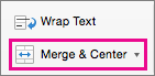
2. Select Merge & Center.

   Important: When you merge multiple cells, the contents of only one cell (the upper-left cell for left-to-right languages, or the upper-right cell for right-to-left languages) appear in the merged cell. The contents of the other cells that you merge are deleted.

Unmerge cells

1. Select the Merge & Center down arrow.

2. Select Unmerge Cells.

Important: 

• You cannot split an unmerged cell. If you are looking for information about how to split the contents of an unmerged cell across multiple cells, see Distribute the contents of a cell into adjacent columns.

• After merging cells, you can split a merged cell into separate cells again. If you don’t remember where you have merged cells, you can use the Find command to quickly locate merged cells.

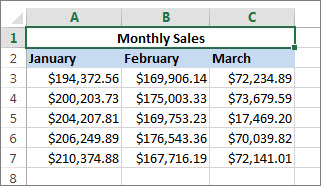
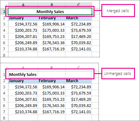
Merging combines two or more cells to create a new, larger cell. This is a great way to create a label that spans several columns.

In the example here, cells A1, B1, and C1 were merged to create the label “Monthly Sales” to describe the information in rows 2 through 7.

Merge cells

Merge two or more cells by following these steps:

1. Select two or more adjacent cells you want to merge.

   Important: Ensure that the data you want to retain is in the upper-left cell, and keep in mind that all data in the other merged cells will be deleted. To retain any data from those other cells, simply copy it to another place in the worksheet—before you merge.

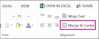
2. On the Home tab, select Merge & Center.
   

Tips: 

• If Merge & Center is disabled, ensure that you’re not editing a cell—and the cells you want to merge aren’t formatted as an Excel table. Cells formatted as a table typically display alternating shaded rows, and perhaps filter arrows on the column headings.

• To merge cells without centering, click the arrow next to Merge and Center, and then click Merge Across or Merge Cells.

Unmerge cells

If you need to reverse a cell merge, click onto the merged cell and then choose Unmerge Cells item in the Merge & Center menu (see the figure above).

Split text from one cell into multiple cells

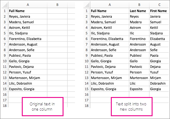
You can take the text in one or more cells, and distribute it to multiple cells. This is the opposite of concatenation, in which you combine text from two or more cells into one cell.

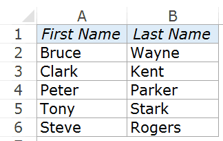
For example, you can split a column containing full names into separate First Name and Last Name columns:

Follow the steps below to split text into multiple columns:

1. Select the cell or column that contains the text you want to split.

2. Note: Select as many rows as you want, but no more than one column. Also, ensure that are sufficient empty columns to the right—so that none of your data is deleted. Simply add empty columns, if necessary.

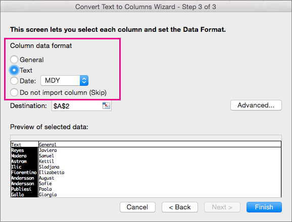
3. Click Data >Text to Columns, which displays the Convert Text to Columns Wizard.

4. Click Delimited > Next.

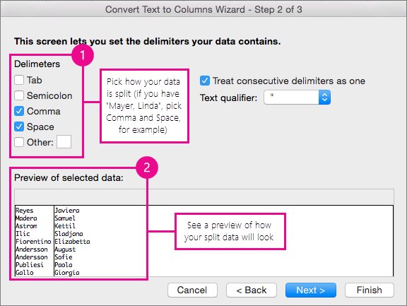
5. Check the Space box, and clear the rest of the boxes. Or, check both the Comma and Space boxes if that is how your text is split (such as «Reyes, Javiers», with a comma and space between the names). A preview of the data appears in the panel at the bottom of the popup window.

   

6. Click Next and then choose the format for your new columns. If you don’t want the default format, choose a format such as Text, then click the second column of data in the Data preview window, and click the same format again. Repeat this for all of the columns in the preview window.
   

7. Click the button to the right of the Destination box to collapse the popup window.

8. Anywhere in your workbook, select the cells that you want to contain the split data. For example, if you are dividing a full name into a first name column and a last name column, select the appropriate number of cells in two adjacent columns.

   

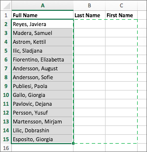
9. Click the button to expand the popup window again, and then click the Finish button.

   

Merging combines two or more cells to create a new, larger cell. This is a great way to create a label that spans several columns. For example, here cells A1, B1, and C1 were merged to create the label “Monthly Sales” to describe the information in rows 2 through 7.

Merge cells

1. Click the first cell and press Shift while you click the last cell in the range you want to merge.

   Important: Make sure only one of the cells in the range has data.

2. Click Home > Merge & Center.

   

   If Merge & Center is dimmed, make sure you’re not editing a cell or the cells you want to merge aren’t inside a table.

   Tip: To merge cells without centering the data, click the merged cell and then click the left, center or right alignment options next to Merge & Center.

   If you change your mind, you can always undo the merge by clicking the merged cell and clicking Merge & Center.

Unmerge cells

To unmerge cells immediately after merging them, press Ctrl + Z. Otherwise do this:

• Click the merged cell and click Home > Merge & Center.

  

  The data in the merged cell moves to the left cell when the cells split.

  

Need more help?

You can always ask an expert in the Excel Tech Community or get support in the Answers community.

See Also

Overview of formulas in Excel

How to avoid broken formulas

Find and correct errors in formulas

Excel keyboard shortcuts and function keys

Excel functions (alphabetical)

Excel functions (by category)

Merged cells are one of the most popular options used by beginner spreadsheet users.

But they have a lot of drawbacks that make them a not so great option.

In this post, I’ll show you everything you need to know about merged cells including 8 ways to merge cells.

I’ll also tell you why you shouldn’t use them and a better alternative that will produce the same visual result.

What is a Merged Cell

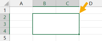
A merged cell in Excel combines two or more cells into one large cell. You can only merge contiguous cells that form a rectangular shape.

The above example shows a single merged cell resulting from merging 6 cells in the range B2:C4.

Why You Might Merge a Cell

Merging cells is a common technique used when a title or label is needed for a group of cells, rows or columns.

When you merge cells, only the value or formula in the top left cell of the range is preserved and displayed in the resulting merged cell. Any other values or formulas are discarded.

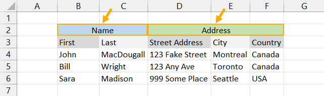
The above example shows two merged cells in B2:C2 and D2:F2 which indicates the category of information in the columns below. For example the First and Last name columns are organized with a Name merged cell.

Why is the Merge Command Disabled?

On occasion, you might find the Merge & Center command in Excel is greyed out and not available to use.

There are two reasons why the Merge & Center command can become unavailable.

• You are trying to merge cells inside an Excel table.
• You are trying to merge cells in a protected sheet.

Cells inside an Excel table can not be merged and there is no solution to enable this.

If most of the other commands in the ribbon are greyed out too, then it’s likely the sheet is protected. In order to access the Merge option, you will need to unprotect the worksheet.

This can be done by going to the Review tab and clicking the Unprotect Sheet command.

If the sheet has been protected with a password, then you will need to enter it in order to unprotect the sheet.

Now you should be able to merge cells inside the sheet.

Merged Cells Only Retain the Top Left Values

Warning before you start merging cells!

If the cells contain data or formulas, then you will lose anything not in the upper left cell.

A warning dialog box will appear telling you Merging cells only keeps the upper-left value and discards other values.

The above example shows the result of merging cells B2:C4 which contains text data. Only the data from cell B2 remains in the resulting merged cells.

If no data is present in the selected cells, then no warning will appear when trying to merge cells.

8 Ways to Merge a Cell

Merging cells is an easy task to perform and there are a variety of places this command can be found.

Merge Cells with the Merge & Center Command in the Home Tab

The easiest way to merge cells is using the command found in the Home tab.

1. Select the cells you want to merge together.
2. Go to the Home tab.
3. Click on the Merge & Center command found in the Alignment section.

Merge Cells with the Alt Hotkey Shortcut

There is an easy way to access the Home tab Merge and Center command using the Alt key.

Press Alt H M C in sequence on your keyboard to use the Merge & Center command.

Merge Cells with the Format Cells Dialog Box

Merging cells is also available from the Format Cells dialog box. This is the menu which contains all formatting options including merging cells.

You can open the Format Cells dialog box a few different ways.

• Go to the Home tab and click on the small launch icon in the lower right corner of the Alignment section.
• Use the Ctrl + 1 keyboard shortcut.
• Right click on the selected cells and choose Format Cells.

Go to the Alignment tab in the Format Cells menu then check the Merge cells option and press the OK button.

Merge Cells with the Quick Access Toolbar

If you use the Merge & Center command a lot, then it might make sense to add it to the Quick Access Toolbar so it’s always readily available to use.

Go to the Home tab and right click on the Merge & Center command then choose Add to Quick Access Toolbar from the options.

This will add the command to your QAT which is always available to use.

A nice bonus that comes with the quick access command is it gets its own hotkey shortcut based on its position in the QAT. When you press the Alt key, Excel will show you what key to press next in order to access the command.

In the above example, the Merge and Center command is the third command in the QAT so the hotkey shortcut is Alt 3.

Merge Cells with Copy and Paste

If you have a merged cell in your sheet already then you can copy and paste it to create more merged cells. This will produce merged cells with the exact same dimensions.

Copy a merged cell using Ctrl + C then paste it into a new location using Ctrl + V. Just make sure the paste area doesn’t overlap an existing merged cell.

Merge Cells with VBA

Sub MergeCells()
    Range("B2:C4").Merge
End Sub

The basic command for merging cells in VBA is quite simple. The above code will merge cells B2:C4.

Merge Cells with Office Scripts

function main(workbook: ExcelScript.Workbook) {
	let selectedSheet = workbook.getActiveWorksheet();
	selectedSheet.getRange("B2:C4").merge(false);
	selectedSheet.getRange("B2:C4").getFormat().setHorizontalAlignment(ExcelScript.HorizontalAlignment.center);
}

The above office script will merge and center the range B2:C4.

Merge Cells inside a PivotTable

We can’t make this change for the selected cells because it will affect a PivotTable. Use the field list to change the report. If you are trying to insert or delete cells, move the PivotTable and try again.

If you try to use the Merge and Center command inside a Pivot Table, you will be greeted with the above error message.

You can’t use the Merge & Center command inside a PivotTable, but there is a way to merge cells in the PivotTable options menu.

In order to avail of this option, you will first need to make sure your Pivot Table is in the tabular display mode.

1. Select a cell inside your PivotTable.
2. Go to the Design tab.
3. Click on Report Layout.
4. Choose Show in Tabular Form.

Your pivot table will now be in the tabular form where each field you add to the Rows area will be in its own column with data in a displayed in a single row.

Now you can enable the option to show merge cells inside the pivot table.

1. Select a cell inside your PivotTable.
2. Go to the PivotTable Analyze tab.
3. Click on Options.

This will open up the PivotTable Options menu.

Enable the Merge and center cells with labels setting in the PivotTable Options menu.

1. Click on the Layout & Format tab.
2. Check the Merge and center cells with labels option.
3. Press the OK button.

Now as you expand and collapse fields in your pivot table, fields will merge when they have a common label.

10 Ways to Unmerge a Cell

Unmerging a cell is also quick and easy. Most methods involve the same steps as used to merge the cell, but there are a few extra methods worth knowing.

Unmerge Cells with the Home Tab Command

This is the same process as merging cells from the Home tab command.

1. Select the merged cells to unmerge.
2. Go to the Home tab.
3. Click on the Merge & Center command.

Unmerge Cells with the Format Cells Menu

You can unmerge cells from the Format Cells dialog box as well.

Press Ctrl + 1 to open the Format Cells menu then go to the Alignment tab then uncheck the Merge cells option and press the OK button.

Unmerge Cells with the Alt Hot Key Shortcut

You can use the same Alt hot key combination to unmerge a merged cell. Select the merged cell you want to unmerge then press Alt H M C in sequence to unmerge the cells.

Unmerge Cells with Copy and Paste

You can copy the format from a regular single cell to unmerge merged cells.

Find a single cell and use Ctrl + C to copy it, then select the merged cells and press Ctrl + V to paste the cell.

You can use the Paste Special options to avoid overwriting any data when pasting. Press Ctrl + Alt + V then select the Formats option.

Unmerge Cells with the Quick Access Toolbar

This is a great option if you have already added the Merge & Center command to the quick access toolbar previously.

All you need to do is select the merged cells and click on the command or use the Alt hot key shortcut.

Unmerge Cells with the Clear Formats Command

Merged cells are a type of format, so it’s possible to unmerge cells by clearing the format from the cell.

1. Select the merged cell to unmerge.
2. Go to the Home tab.
3. Click on the right part of the Clear button found in the Editing section.
4. Select Clear Formats from the options.

Unmerge Cells with VBA

Sub UnMergeCells()
    Range("B2:C4").UnMerge
End Sub

Above is the basic command for unmerging cells in VBA. This will unmerge cells B2:C4.

Unmerge Cells with Office Scripts

Most methods of merging a cell can be performed again to unmerge cells like a toggle switch to merge or unmerge.

However the code in office scripts doesn’t work like this and instead, you will need to remove formatting to unmerge.

function main(workbook: ExcelScript.Workbook) {
	let selectedSheet = workbook.getActiveWorksheet();
	selectedSheet.getRange("B2:C4").clear(ExcelScript.ClearApplyTo.formats);
}

The above code will clear the format in cells B2:C4 and unmerge any merged cells it contains.

Unmerge Cells with the Accessibility Pane

Merged cells create problems for screen readers which is an accessibility issue. Because of this, they are flagged in the Accessibility window pane.

If you know the location of the merged cells, you can select them and go to the Review tab then click on the lower part of the Check Accessibility button and choose Unmerge Cells.

If you don’t know where all the merged cells are, you can open up the accessibility pane and it will show you where there are and you will be able to unmerge them one by one.

Go to the Review tab and click on the top part of the Check Accessibility command to launch the accessibility window pane.

This will show a Merged Cells section which you can expand to see all merged cells in the workbook. Click on the address and Excel will take you to that location.

Click on the downward chevron icon to the right of the address and the Unmerge option can be selected.

Unmerge Cells inside a PivotTable

To unmerge cells inside a pivot table, you just need to disable the setting in the pivot table options menu.

Now you can enable the option to show merge cells inside the pivot table.

1. Select a cell inside your PivotTable.
2. Go to the PivotTable Analyze tab.
3. Click on Options.
4. Click on the Layout & Format tab.
5. Uncheck the Merge and center cells with labels option.
6. Press the OK button.

Merge Multiple Ranges in One Step

In Excel, you can select multiple non-continuous ranges in a sheet by holding the Ctrl key. A nice consequence of this is you can convert these multiple ranges into merged cells in one step.

Hold the Ctrl key while selecting multiple ranges with the mouse. When you’re finished selecting the ranges you can release the Ctrl key and then go to the Home tab and click on the Merge & Center command.

Each range will become its own merged cell.

Combine Data Before Merging Cells

Before you merge any cells which contain data, it’s advised to combine the data since only the data in the top left cell is preserved when merging cells.

There are a variety of ways to do this, but using the TEXTJOIN function is among the easiest and most flexible as it will allow you to separate each cell’s data using a delimiter if needed.

= TEXTJOIN ( ", ", TRUE, B2:C4 )

The above formula will join all the text in range B2:C4 going from left to right and then top to bottom. Text in each cell is separated with a comma and space.

Once you have the formula result, you can copy and paste it as a value so that the data is retained when you merge the cells.

How to Get Data from Merged Cells in Excel

A common misconception is that each cell of in the merged range contains the data entered inside.

In fact, only the top left cell will contain any data.

In the above example, the formula references the top left value in the merged range. The result returned is what is seen in the merged range.

In this example, the formula references a cell that is not the top left most cell in the merged range. The result is 0 because this cell is empty and contains no value.

In order to extract data from a merged range, you will always need to reference the top left most cell of the range. Fortunately, Excel automatically does this for you when you select the merged cell in a formula.

How to Find Merged Cells in a Workbook

If you create a bunch of merged cells, you might need to find them all later. Thankfully it’s not a painful process.

This can be done using the Find & Select command.

Go to the Home tab and click on the Find & Select button found in the Editing section, then choose the Find option. This will open the Find and Replace menu

You can also use the Ctrl + F keyboard shortcut.

You don’t need to enter any text to find, you can use this menu to find cells formatted as merged cells.

1. Click on the Format button to open the Find Format menu.
2. Go to the Alignment tab.
3. Check the Merge cells option.
4. Press the OK button in the Find Format menu.
5. Press the Find All or Find Next button in the Find and Replace menu.

Unmerge All Merged Cells

Fortunately, unmerging all merged cells in a sheet is very easy.

1. Select the entire sheet. You can do this two ways.
   • Click on the select all button where the column headings meet the row headings.
   • Press Ctrl + A on your keyboard.
2. Go to the Home tab.
3. Press the Merge & Center command.

This will unmerge all the merged cells and leave all the other cells unaffected.

Why You Shouldn’t Merge Cells

There are a lot of reasons why you shouldn’t merge cells.

• You can’t sort data with merged cells.
• You can’t filter data with merged cells.
• You can’t copy and paste values into merged cells.
• It will create accessibility problems for screen readers by changing the order in which text should be read.

This isn’t an exhaustive list, there are likely many more you will come across should you choose to merge cells.

Alternative to Merging a Cell

Good news!

There is a much better alternative than merging cells.

This alternative has none of the negative features that come with merging cells but will still allow you to achieve the same visual look of a merged cell.

It will allow you to display text centered across a range of cells without merging the cells.

Unfortunately, this technique will only work horizontally with one row of cells. There is no option to do something similar with a vertical range of cells.

Select the horizontal range of cells that you would like to center your text across. The first cell should contain the text which is to be centered while the remaining cells should be empty.

This example shows text in cell B2 and the range B2:C2 is selected as the range to center across.

Go to the Home tab and click on the small launch icon in the lower right corner of the Alignment section. This will open up the Format Cells dialog box with the Alignment tab active.

You can also press Ctrl + 1 to open the Format Cells dialog box and navigate to the Alignment tab.

Select Center Across Selection from the Horizontal dropdown options in the Text alignment section.

The text will now appear as though it occupies all cells but it will only exist in the first cell of the centering selection and each cell is still separate.

Pros

• The text appears centered across the selected range similar to a merged cell.
• No negative effects from merged cells.
• Can be used inside an Excel table.

Cons

• Can not center across a vertical range of cells.

Conclusions

There are lots of ways to merge cells in Excel. You can also easily unmerge cells too if you need to.

There are many things to consider when merging cells in Excel.

As you have seen, there are lots of pitfalls to merged cells that you should consider before implementing them in your workbooks.

Do you have a favorite merge method or warning about the dangers of merged cells that are not listed in the post? Let me know about it in the comments.

Watch Video – Combine cells in Excel (using Formulas)

A lot of times, we need to work with text data in Excel. It could be Names, Address, Email ids, or other kinds of text strings. Often, there is a need to combine cells in Excel that contain the text data.

Your data could be in adjacent cells (rows/columns), or it could be far off in the same worksheet or even a different worksheet.

How to Combine Cells in Excel

In this tutorial, you’ll learn how to Combine Cells in Excel in different scenarios:

• How to Combine Cells without Space/Separator in Between.
• How to Combine Cells with Space/Separator in Between.
• How to Combine Cells with Line Breaks in Between.
• How to Combine Cells with Text and Numbers.

How to Combine Cells without Space/Separator

This is the easiest and probably the most used way to combine cells in Excel. For example, suppose you have a data set as shown below:

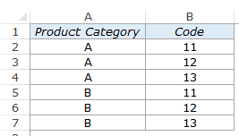
You can easily combine cells in columns A and B to get a string such as A11, A12, and so on..

Here is how you can do this:

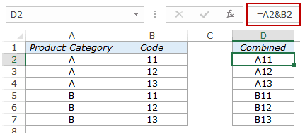
• Enter the following formula in a cell where you want the combined string:

  =A2&B2

• Copy-paste this in all the cells.

This will give you something as shown below:

You can also do the same thing using the CONCATENATE function instead of using the ampersand (&). The below formula would give the same result:

=CONCATENATE(A2,B2)

How to Combine Cells with Space/Separator in Between

You can also combine cells and have a specified separator in between. It could be a space character, a comma, or any other separator.

Suppose we have a dataset as shown below:

Here are the steps to combine the first and the last name with a space character in between:

• Enter the following formula in a cell:

  =A2&" "&B2

• Copy-paste this in all the cells.

This would combine the first name and last name with a space character in between.

If you want any other separator (such as comma, or dot), you can use that in the formula.

How to Combine Cells with Line Breaks in Between

Apart from separators, you can also add line breaks while you combine cells in Excel.

Suppose you have a dataset as shown below:

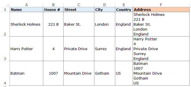
In the above example, different parts of the address are in different cells (Name, House #, Street, City, and Country).

You can use the CONCATENATE function or the & (ampersand) to combine these cells.

However, just by combining these cells would give you something as shown below:

This is not in a good address format. You can try using the text wrap, but that wouldn’t work either.

What is needed here is to have each element of the address on a separate line in the same cell. You can achieve that by using the CHAR(10) function along with the & sign.

CHAR(10) is a line feed in Windows, which means that it forces anything after it to go to a new line.

Use the below formula to get each cell’s content on a separate line within the same cell:

=A2&CHAR(10)&B2&CHAR(10)&C2&CHAR(10)&D2&CHAR(10)&E2

This formula uses the CHAR(10) function in between each cell reference and inserts a line break after each cell. Once you have the result, apply wrap text in the cells that have the results and you’ll get something as shown below:

How to Combine Cells with Text and Numbers

You can also combine cells that contain different types of data. For example, you can combine cells that contain text and numbers.

Let’s have a look at a simple example first.

Suppose you have a dataset as shown below:

The above data set has text data in one cell and a number is another cell. You can easily combine these two by using the below formula:

=A2&"-"&B2

Here I have used a dash as the separator.

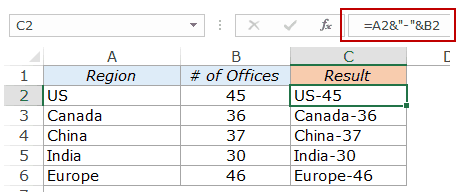
You can also add some text to it. So you can use the following formula to create a sentence:

=A2&" region has "&B2&" offices"

Here we have used a combination of cell reference and text to construct sentences.

Now let’s take this example forward and see what happens when you try and use numbers with some formatting applied to it.

Suppose you have a dataset as shown below, where we have sales values.

Now let’s combine the cells in Column A and B to construct a sentence.

Here the formula I’ll be using:

=A2&" region generated sales of "&B2

Here is how the results look like:

Do you see the problem here? Look closely at the format of the sales value in the result.

You can see that the formatting of the sales value goes away and the result has the plain numeric value. This happens when we combine cells with numbers that have formatting applied to it.

Here is how to fix this. Use the below formula:

=A2&" region generated sales of "&TEXT(B2,"$ ###,0.0")

In the above formula, instead of using B2, we have used the TEXT function. TEXT function makes the number show up in the specified format and as text. In the above case, the format is $ ###,0.0. This format tells Excel to show the number with a dollar sign, a thousand-separator, and one decimal point.

Similarly, you can use the Text function to show in any format allowed in Excel.

Here is another example. There are names and date of birth, and if you try and combine these cells, you get something as shown below:

You can see that Excel completely screws up the date format. The reason is that date and time are stored as numbers in Excel, and when you combine cells that have numbers, as shown above, it shows the number value but doesn’t use the original format.

Here is the formula that will fix this:

=A2&" was born on "&TEXT(B2,"dd mmm yyy")

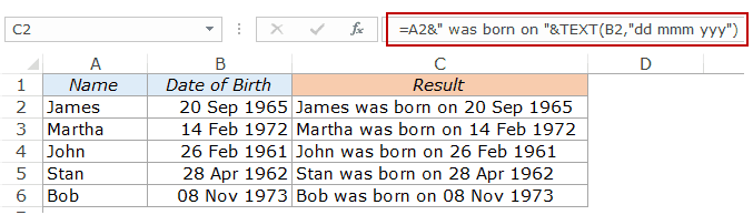
Again, here we have used the TEXT function and specified the format in which we want the Date of Birth to show up in the result.

Here is how this date format works:

• dd – Shows the day number of the date. (try using ddd and see what happens).
• mmm – shows the three-letter code for a month.
• yyy – shows the year number.

Cool… Isn’t it?

Let me know your thoughts in the comments section.

You May Also Like the Following Excel Tutorials:

• CONCATENATE Excel Range (with and without separator).
• How to Merge Cells in Excel the Right Way.
• How to Combine Multiple Workbooks into One Excel Workbook.
• How to Combine Data from Multiple Workbooks into One Excel Table (using Power Query).
• How to Merge Cells in Excel
• How to Combine Duplicate Rows and Sum the Values in Excel
• Combine Date and Time in Excel

Combining values with CONCATENATE is the best way, but with this function, it’s not possible to refer to an entire range.

You need to select all the cells of a range one by one, and if you try to refer to an entire range, it will return the text from the first cell.

In this situation, you do need a method where you can refer to an entire range of cells to combine them in a single cell.

So today in this post, I’d like to share with you 5 different ways to combine text from a range into a single cell.

[CONCATENATE + TRANSPOSE] to Combine Values

The best way to combine text from different cells into one cell is by using the transpose function with concatenating function.

Look at the below range of cells where you have a text but every word is in a different cell and you want to get it all in one cell.

Below are the steps you need to follow to combine values from this range of cells into one cell.

1. In the B8 (edit the cell using F2), insert the following formula, and do not press enter.
   • =CONCATENATE(TRANSPOSE(A1:A5)&” “)
2. Now, select the entire inside portion of the concatenate function and press F9. It will convert it into an array.
3. After that, remove the curly brackets from the start and the end of the array.
4. In the end, hit enter.

That’s all.

How this formula works

In this formula, you have used TRANSPOSE and space in the CONCATENATE. When you convert that reference into hard values it returns an array.

In this array, you have the text from each cell and a space between them and when you hit enter, it combines all of them.

Combine Text using the Fill Justify Option

Fill justify is one of the unused but most powerful tools in Excel. And, whenever you need to combine text from different cells you can use it.

The best thing is, that you need a single click to merge text. Have look at the below data and follow the steps.

1. First of all, make sure to increase the width of the column where you have text.
2. After that, select all the cells.
3. In the end, go to Home Tab ➜ Editing ➜ Fill ➜ Justify.

This will merge text from all the cells into the first cell of the selection.

TEXTJOIN Function for CONCATENATE Values

If you are using Excel 2016 (Office 365), there is a function called “TextJoin”. It can make it easy for you to combine text from different cells into a single cell.

Syntax:

TEXTJOIN(delimiter, ignore_empty, text1, [text2], …)

1. delimiter a text string to use as a delimiter.
2. ignore_empty true to ignore blank cell, false to not.
3. text1 text to combine.
4. [text2] text to combine optional.

how to use it

To combine the below list of values you can use the formula:

=TEXTJOIN(" ",TRUE,A1:A5)

Here you have used space as a delimiter, TRUE to ignore blank cells and the entire range in a single argument. In the end, hit enter and you’ll get all the text in a single cell.

Combine Text with Power Query

Power Query is a fantastic tool and I love it. Make sure to check out this (Excel Power Query Tutorial). You can also use it to combine text from a list in a single cell. Below are the steps.

1. Select the range of cells and click on “From table” in data tab.
   
2. If will edit your data into Power Query editor.
   
3. Now from here, select the column and go to “Transform Tab”.
4. From “Transform” tab, go to Table and click on “Transpose”.
   
5. For this, select all the columns (select first column, press and hold shift key, click on the last column) and press right click and then select “Merge”.
   
6. After that, from Merge window, select space as a separator and name the column.
   
7. In the end, click OK and click on “Close and Load”.

Now you have a new worksheet in your workbook with all the text in a single cell. The best thing about using Power Query is you don’t need to do this setup again and again.

When you update the old list with a new value you need to refresh your query and it will add that new value to the cell.

VBA Code to Combine Values

If you want to use a macro code to combine text from different cells then I have something for you. With this code, you can combine text in no time. All you need to do is, select the range of cells where you have the text and run this code.

 Sub combineText()
 Dim rng As Range
 Dim i As String
 For Each rng In Selection
 i = i & rng & " "
 Next rng
 Range("B1").Value = Trim(i)
 End Sub 

Make sure to specify your desired location in the code where you want to combine the text.

In the end,

There may be different situations for you where you need to concatenate a range of cells into a single cell. And that’s why we have these different methods.

All methods are easy and quick, you need to select the right method as per your need. I must say that give a try to all the methods once and tell me:

Which one is your favorite and worked for you?

Please share your views with me in the comment section. I’d love to hear from you, and please, don’t forget to share this post with your friends, I am sure they will appreciate it.