
Auto number a column by AutoFill function Type 1 into a cell that you want to start the numbering, then drag the autofill handle at the right-down corner of the cell to the cells you want to number, and click the fill options to expand the option, and check Fill Series, then the cells are numbered.
Contents
- 1 How do I number multiple columns in Excel?
- 2 How do you label Excel columns with numbers?
- 3 How do you create a number sequence in Excel without dragging?
- 4 How do I change a number to a percent in Excel?
- 5 How do I show columns and row numbers in Excel?
- 6 How do I add a numbered column in numbers?
- 7 How do I make a numbered list in numbers?
- 8 How do I apply a formula to an entire column in numbers?
- 9 How do I change the order of columns in Excel?
- 10 How do you auto fill columns in Excel?
- 11 How do you make a number into a percent?
- 12 How do you change a number back to a percentage?
- 13 How do you change a number into percentage?
- 14 How do you show columns in Excel?
- 15 Why can’t I see Row numbers in Excel?
- 16 How are columns labeled in an Excel worksheet?
- 17 How do I add numbers in columns in pages?
- 18 What is a numbered list?
- 19 How do I create a list style in pages?
- 20 How do you format a list?
Fill a column with a series of numbers
- Select the first cell in the range that you want to fill.
- Type the starting value for the series.
- Type a value in the next cell to establish a pattern.
- Select the cells that contain the starting values.
- Drag the fill handle.
How do you label Excel columns with numbers?
To change the column headings to letters, select the File tab in the toolbar at the top of the screen and then click on Options at the bottom of the menu. When the Excel Options window appears, click on the Formulas option on the left. Then uncheck the option called “R1C1 reference style” and click on the OK button.
How do you create a number sequence in Excel without dragging?
The regular way of doing this is: Enter 1 in cell A1. Enter 2 in cell A2. Select both the cells and drag it down using the fill handle.
Quickly Fill Numbers in Cells without Dragging
- Enter 1 in cell A1.
- Go to Home –> Editing –> Fill –> Series.
- In the Series dialogue box, make the following selections:
- Click OK.
How do I change a number to a percent in Excel?
How to Apply the Percent Number Format in Excel 2010
- Select the cells containing the numbers you want to format.
- On the Home tab, click the Number dialog box launcher in the bottom-right corner of the Number group.
- In the Category list, select Percentage.
- Specify the number of decimal places.
- Click OK.
How do I show columns and row numbers in Excel?
On the Ribbon, click the Page Layout tab. In the Sheet Options group, under Headings, select the Print check box. , and then under Print, select the Row and column headings check box .
How do I add a numbered column in numbers?
Click the table. in the top-right corner of the table to add a column, or drag it to add or delete multiple columns. You can delete a row or column only if all of its cells are empty.
How do I make a numbered list in numbers?
Select the list items with the numbering or lettering you want to change. In the Format sidebar, click the Text tab, then click the Style button near the top of the sidebar. Click the disclosure arrow next to Bullets & Lists, then click the pop-up menu below Bullets & Lists and choose Numbers.
How do I apply a formula to an entire column in numbers?
Select that cell. You will see a small circle in the bottom-right corner of the cell. Click and drag that down and all cells below will auto-fill with the number 50 (or a formula if you have that in a cell). Works in a fill-right direction too.
How do I change the order of columns in Excel?
To quickly move columns in Excel without overwriting existing data, press and hold the shift key on your keyboard.
- First, select a column.
- Hover over the border of the selection.
- Press and hold the Shift key on your keyboard.
- Click and hold the left mouse button.
- Move the column to the new position.
How do you auto fill columns in Excel?
Click and hold the left mouse button, and drag the plus sign over the cells you want to fill. And the series is filled in for you automatically using the AutoFill feature. Or, say you have information in Excel that isn’t formatted the way you need it to be, such as this list of names.
How do you make a number into a percent?
To turn a percent into an integer or decimal number, simply divide by 100. That is the same as moving the decimal point two places to the left.
How do you change a number back to a percentage?
Step 1) Get the percentage of the original number. If the percentage is an increase then add it to 100, if it is a decrease then subtract it from 100. Step 2) Divide the percentage by 100 to convert it to a decimal. Step 3) Divide the final number by the decimal to get back to the original number.
How do you change a number into percentage?
Percentage Change | Increase and Decrease
- First: work out the difference (increase) between the two numbers you are comparing.
- Increase = New Number – Original Number.
- Then: divide the increase by the original number and multiply the answer by 100.
- % increase = Increase ÷ Original Number × 100.
How do you show columns in Excel?
How to show hidden columns that you select
- Select the columns to the left and right of the column you want to unhide. For example, to show hidden column B, select columns A and C.
- Go to the Home tab > Cells group, and click Format > Hide & Unhide > Unhide columns.
Why can’t I see Row numbers in Excel?
Step 1 – Click on “View” Tab on Excel Ribbon. Step 3 – Uncheck “Headings” checkbox to hide Excel worksheet Row and Column headings. Check “Headings” checkbox to show missing hidden Excel worksheet Row and Column headings, as explained in below image.
How are columns labeled in an Excel worksheet?
How are columns and rows labeled? In all spreadsheet programs including Microsoft Excel, rows are labeled using numbers (e.g., 1 to 1,048,576). All columns are labeled with letters starting with the letter A and then incrementing by a letter after the final letter Z.
How do I add numbers in columns in pages?
Inserting columns in Pages
- 1) Open your document or create a new one in Pages.
- 2) Click the Format button on the top right to open the formatting sidebar.
- 3) Click the Layout button and you should see the Columns settings right below it.
- 4) Use the arrows or pop in a number for the number of columns you want to insert.
What is a numbered list?
Numbered-list meaning. Filters. A list whose items are numbered, with various styles including Arabic numerals and Roman numerals. noun. 5.
How do I create a list style in pages?
In the Format sidebar, click the Style button near the top. If the text is in a text box, table, or shape, first click the Text tab at the top of the sidebar, then click the Style button. Click the pop-up menu next to Bullets & Lists, then choose a list style.
How do you format a list?
Format for Lists
- Use a colon to introduce the list items only if a complete sentence precedes the list.
- Use both opening and closing parentheses on the list item numbers or letters: (a) item, (b) item, etc.
- Use either regular Arabic numbers or lowercase letters within the parentheses, but use them consistently.
Bottom Line: Learn 4 different techniques for creating a list of numbers in Excel. These include both static and dynamic lists that change when items are added or deleted from the list.
Skill Level: Beginner
Watch the Tutorial
Download the Excel File
You can download the worksheet that I use in the video here:
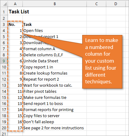
If you have a list of items in Excel and you’d like to insert a column that numbers the items, there are several ways to accomplish this. Let’s look at four of those ways.
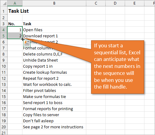
1. Create a Static List Using Auto-Fill
The first way to number a list is really easy. Start by filling in the first two numbers of your list, select those two numbers, and then hover over the bottom right corner of your selection until your cursor turns into a plus symbol. This is the fill handle.
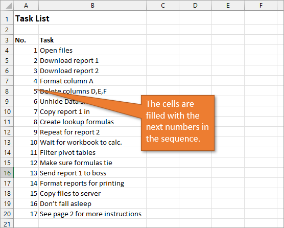
When you double-click on that fill handle (or drag it down to the end of your list), Excel will fill in the blanks with the next numbers in the sequence.
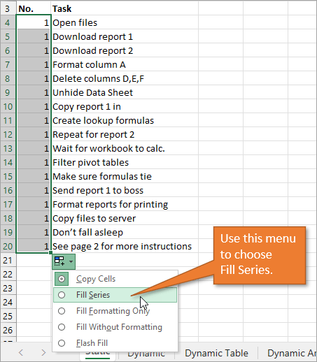
An alternate way to create this same numbered list is to type a 1 in the first cell and then double-click the fill handle. Because Excel doesn’t have a second number to identify a sequence or pattern, it will fill down the columns with 1s. But you will notice that a menu is available at the end of your column, and from that menu, you can select the option to Fill Series. This will change the 1s to a sequential list of numbers.
The numbered column we’ve created in both instances is static. This means it doesn’t change when you make additions or deletions to the corresponding list of items. For example, if I insert a new row in order to add another task, there is a break in the numbered column as well, and I would have to repeat the same steps to correct the list.
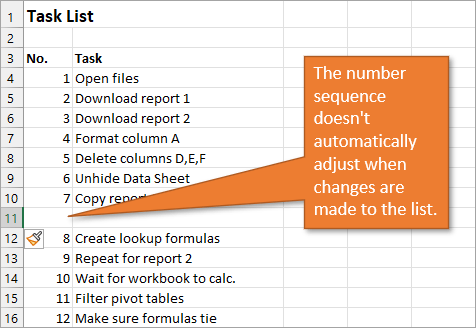
So, unless we want the numbers to always remain as they are, a better option would be to create a dynamic list.
2. Create a Dynamic List Using a Formula
We can use formulas to create a dynamic list where the numbers update when we add or delete rows from the list.
To use a formula for creating a dynamic number list, we can use the ROW function. The ROW function returns the row number of a cell. If we don’t specify a cell for ROW, it just returns the current row number of whatever is selected.
In our example, the first cell in our list doesn’t start on Row 1. It starts on Row 4. But we don’t want our list to start at 4; we want it to start at 1. To subtract the extra 3, our formula will include a minus sign and then the ROW function again, but this time pointed to the cell above our formula (which is in Row 3).
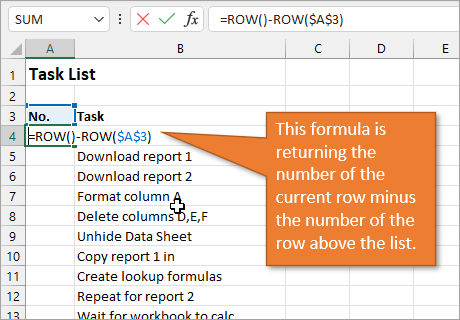
We use the absolute values (dollar signs) in our cell selection because we don’t want that number to change as we copy the formula down the list. In other words, we always want to subtract 3 from the row number to give us our list number.
When we copy down the formula, we have a numbered list that will adjust when we add or delete rows. However, when adding a row, we will have to copy the formula into the newly inserted cell.
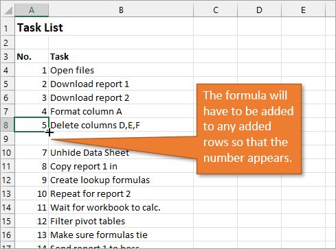
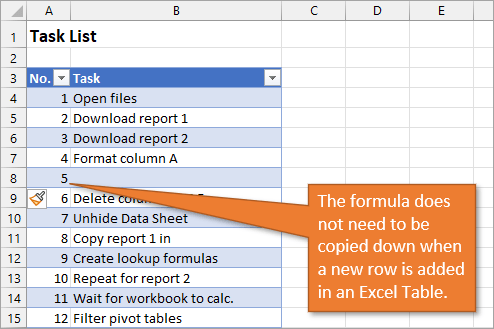
This additional step of copying the formula into new rows can be avoided if we use Excel Tables.
3. Create a Dynamic List Using a Formula in an Excel Table
If we write the same formula but we use an Excel table, the only difference we will make in the formula is that we reference the column header instead of the absolute cell value.
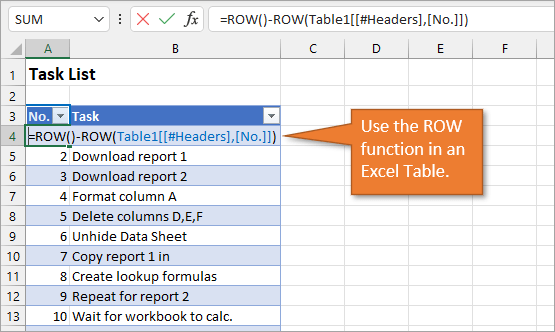
Because we are using an Excel Table, the formula automatically fills down to the other rows. When we add a row to the table, the formula will automatically populate in the new cell.
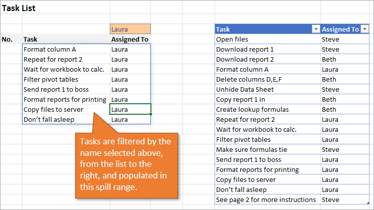
4. Create a Dynamic List Using Dynamic Array Formulas
Below, I have a table that is populated using Dynamic Array Formulas. The FILTER formula spills a range of results based on whatever name is selected in the orange cell.
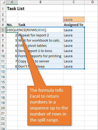
The Dynamic Array formula we will use is SEQUENCE. This will return a sequence for the number of rows we identify in the formula. To tell Excel how many rows there are, we will use the ROW function as the argument for sequence. The argument for ROW is just the spill range. The way to notate the spill range is to simply place a hashtag after the name of the first cell in the range. So our formula looks like this:
=SEQUENCE(ROWS(B5#))
Once we complete our formula and hit Enter, the list will be numbered.
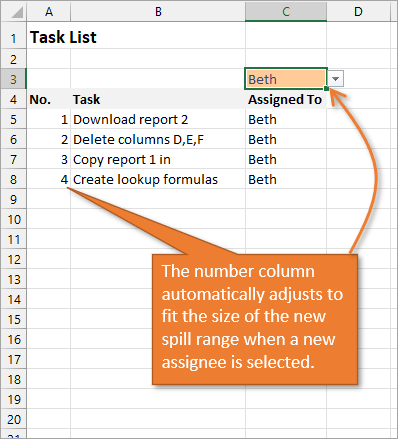
With this formula in place, if the size of the range changes when a new name is selected, the numbered column for the list will automatically adjust as well.
Bonus Tip: Formatting Your Numbered List
If you want to add periods or other punctuation to your numbered list:
- Select the entire list and right-click to choose Format Cells. Or use the keyboard shortcut Ctrl + 1.
- Choose the Custom option on the Number tab.
- Then in the Type field, type in the number 0 with whatever punctuation you would like to surround your number.
Here, I’ve just added a period.
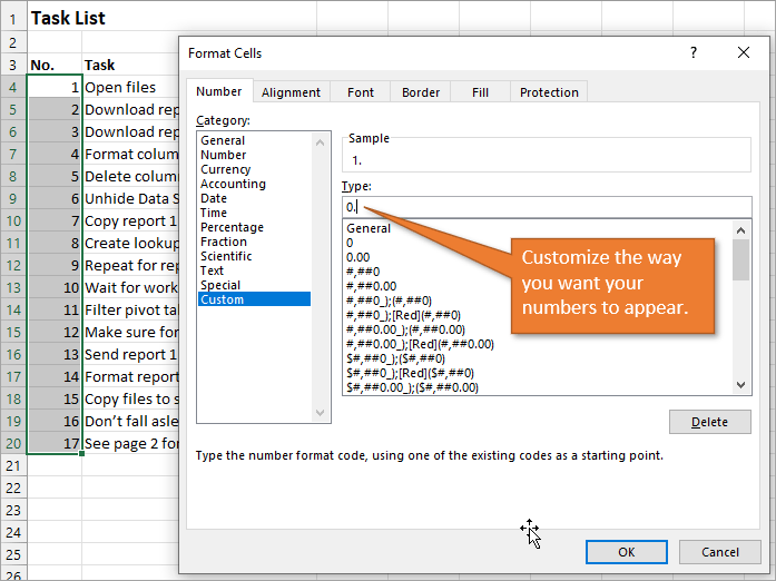
When you hit OK, you will have formatted the entire selection.
Related Posts
Here are a few similar posts that may interest you.
- Excel Tables Tutorial Video – Beginners Guide for Windows & Mac
- New Excel Features: Dynamic Array Formulas & Spill Ranges
- How to Prevent Excel from Freezing or Taking A Long Time when Deleting Rows
Conclusion
I hope these four ways to create ordered lists are helpful for you. If you have questions or feedback, I would love to hear them in the comments. Have a great week!
Have you ever opened an Excel workbook and found that the column headings show numbers instead of letters? The formula look strange too, showing references like RC[-1] instead of D2.

This is R1C1 reference style — a handy feature, and I use it sometimes when programming or setting up a workbook.
Numbers on the column headings make it easier to set up formulas that need a column number, such as VLOOKUP. I don’t have to get fingerprints on my screen, as I count across to column R, where the lookup value is.
Video: Change Excel Column Headings from Numbers to Letters
To see why this happens, and how to switch the column headings back to letters, watch this short video tutorial. The written instructions are below the video.
Your browser can’t show this frame. Here is a link to the page
Why It Happens
Maybe you’ve never heard of R1C1 reference style, and certainly didn’t change any settings. If you didn’t turn that option on, why did the numbers suddenly appear? Probably because someone sent you a workbook, and that’s the first Excel file that you opened today.
The first workbook that you open, when opening Excel, sets the reference style. For example, perhaps I built a workbook for you, and saved it while I was using R1C1 reference style.
I sent you the workbook overnight, and it was the first thing you opened this morning. Surprise! There are numbers in the column headings.
Turn R1C1 Reference Style On or Off
If you close Excel, then open a workbook that you created yourself, with letters in the column headings, that will change the reference style back to A1, which has letters in the column headings.
Or, to manually change the reference style, you can change the option setting.
In Excel 2010:
- At the left end of the Ribbon, click the File tab, then click Options.
- Click the Formulas category.
- In the Working with Formulas section, add or remove the check mark from ‘R1C1 reference style’
- Click OK to close the Options window.

In Excel 2007:
-
- At the left end of the Ribbon, click the Office Button, then click Excel Options.
- Click the Formulas category.
- In the Working with Formulas section, add or remove the check mark from ‘R1C1 reference style’
- Click OK to close the Options window.
In Excel 2003 and earlier versions:
- On the Tools menu, click Options and select the General tab.
- Add or remove the check mark from ‘R1C1 reference style’
- Click OK to close the Options dialog box.

Use a Macro to Switch Headings
If you frequently change the headings from numbers to letters, or letters to numbers, you can create a macro to do the work for you.
There are instructions in this blog post: Excel VBA: Switch Column Headings to Numbers
________________________
Adding numbers in a column or on a row is one of the most basic Excel Functions. Here are 3 easy ways to do it.
- Use simple addition ( the plus sign +)
- Use the SUM() function
- Use the AUTOSUM button
Simple addition
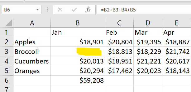
In the example below we have a list of cells containing the amount of money in sales for 12 months for 4 products. Assuming that we want to add all the amounts in January, let’s do a simple addition of the 4 numbers highlighted.
How to create a simple addition
A simple addition looks like this: Total = B2 + B3+ B4+ B5
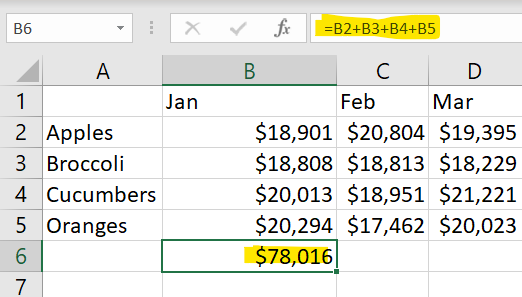
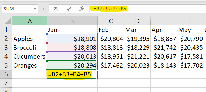
The Excel Formula is built as you type or as you select each cell to be added.
How to build up the addition formula
Here are the steps:
- type =
- select B2
- type +
- select B3
- type +
- select B4
- type +
- select B5
- Type Enter
Alternatively, you can type the entire formula using your keyboard
=B2+B3+B4+B5 (type Enter to calculate the formula)
Notice how the cells in the formula are highlighting as you type. To identify the cells, Excel uses a different color for each one.
When you press Enter, the formula is calculating the result and Excel is displaying it in the B6 cell (or wherever you typed the formula):
What happens when you add empty cells
If one or more of the cells are empty, Excel will consider them zero.
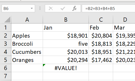
What happens if you add cells that are not numbers
If one or more of the cells are not a number, the formula will result in an error
As any Excel formulas, the result will always show the current value of the addition of these cells.
Any time you change one of the values in the added cells, the result will change immediately to show the correct sum of these cells.
How to build the formula using the mouse
Here is how you do the addition using the mouse to point at the cells as you add.
- Click on the cell where you want the result of the calculation to appear (B6)
- Type = (press the “equals” (=) key to start writing your formula)
- Click on the first cell to be added (B2)
- Type + (that’s the plus sign)
- Click on the second cell to be added (B3)
- Type + again, and the next cell to be added.
- Repeat until all cells to be added have been clicked.
- Press Enter.
This will create the same addition formula as above without the manual typing.
Only use this approach for a limited number of cells due to the difficulty of keeping track of all the cells to be added.
Use the next method (the SUM() function) for a larger set of numbers.
Use the SUM() function to add up numbers in a column
The SUM() function is a more efficient way to add up cells.
You can use the SUM function to add up individual cells, or to add up a range of cells simply by specifying the first and last cell in a range of cells to be added up.
The SUM() function will add up the values in all the cells between the start cell and the end cell in the shortest path possible.
It becomes very useful when adding hundreds, or thousands of cells. Excel has over 1,000,000 rows so imaging typing that many cells into an addition. It is much easier to type a formula like SUM (A1:A1000000)
How to use the SUM() function
If you look at the earlier example, you could use SUM() as shown in the screenshot to achieve the same result.
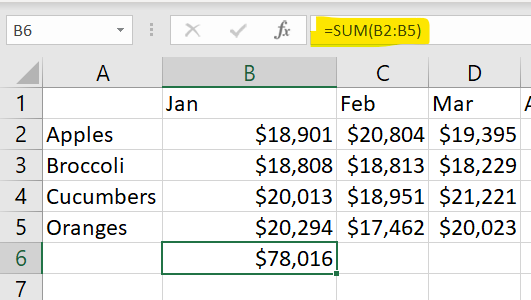
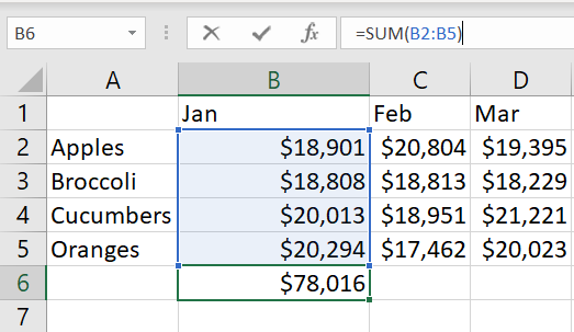
Notice how the cells included in the formula are highlighted just like in the addition case above.
However, in this case, a range is highlighted from the first cell to the last cell specified. This is a useful way to check whether your formula is using the correct range for the SUM.

This formula adds up all the cells from B2 to B5 inclusive. This method can be used just as easily to add up several thousands of cells in a row or column, as well as a set of rows or a set of columns.
Add numbers in a column (B2 to B5)
In the example below, the SUM function is adding numbers in a column. As you type the formula, observe the blue mark showing you the range that is added.
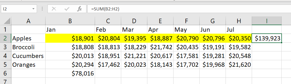
Add numbers in a row (B2 to H2)
In the screenshot below, the same function can be used to sum up the values in a row.
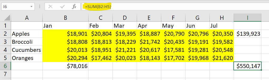
Several rows and columns (all rows and columns B2 to H5)
In the next example, Excel is adding all the values in an array.
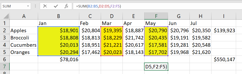
Multiple ranges
You can use SUM to add numbers in multiple ranges (only the months of January, March and May). Press CTRL while selecting all the ranges needed with the mouse.

While you type, notice the Range is highlighted so that you are aware of what is being added in the formula.
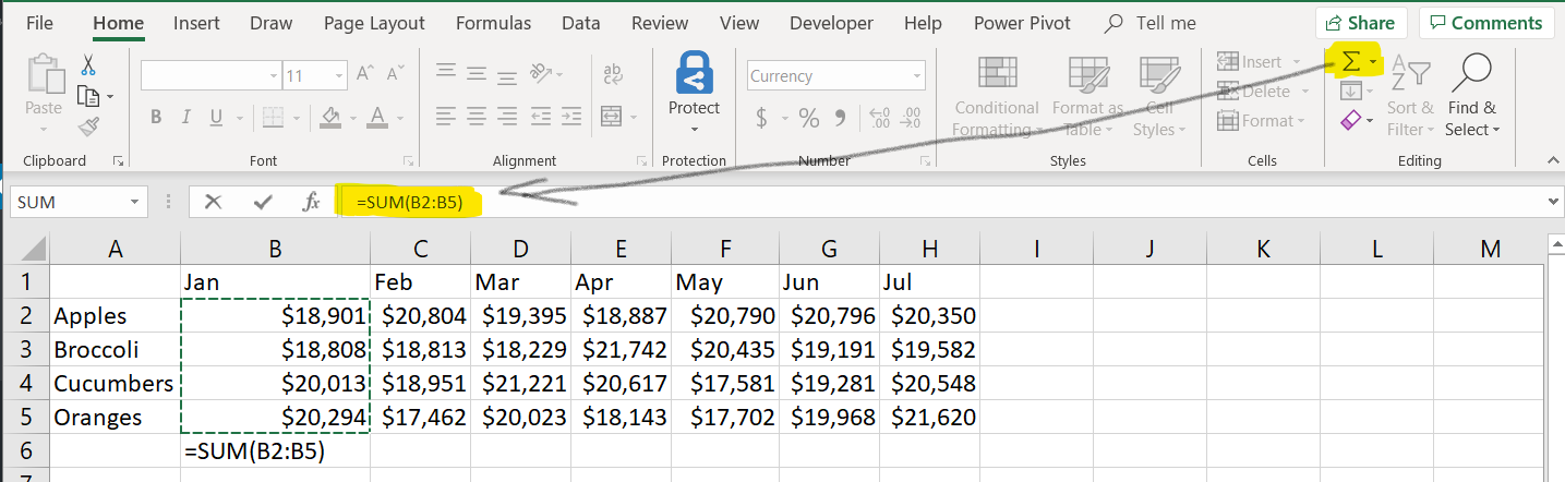
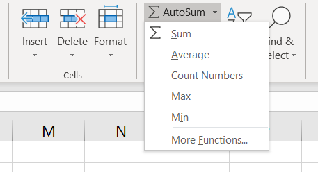
The AUTOSUM button
The last and most efficient method to sum up numbers in a row or column is to use the AUTOSUM button.
This button will use Excel artificial intelligence to evaluate your data set. If your selection is on the first empty cell under a column when you press the AUTOSUM button, Excel will assume that you want to add all the numbers in that column and place the result in the empty cell. This is what 99% of users do. This method saves even more time in typing additions or SUM formulas but just pressing one button.
Where can I find the AUTOSUM button
Autosum is in the Home tab, in the Editing subsection

Modify the resulting formula as you like to reduce or increase the range of numbers.
There are other function under the Autosum dropdown that you can use. You can calculate the average of your numbers, count them, pick the minimum or the maximum and even explore other numerical functions.
These are the three ways Excel can add numbers on a column or row.
By default, the reference style for the cells in Excel are in A1 format, where columns are labeled with letters and rows with numbers.
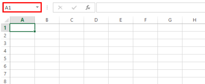 Figure 1. Name box displaying the cell address “A1”
In the image above, the top left cell has a cell reference of A1, as shown in the name box just above it. A1 means column A and row 1. The cell to its right is B1, then C1, and so on up to column XFD.
When we enter the formula =CELL(“address”,A1) into cell A1 and copy the formula down to G7, we will be able to display the cell address of cells A1:G7.
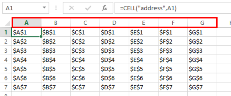 Figure 2. Column labels are letters in A1 style
Show column number
In order to show column number on the label instead of letters, we change the cell reference style to R1C1 by following these steps:
- Click File tab > Options
- In the Excel Options dialog box, select Formulas and check R1C1 reference style
- Click OK
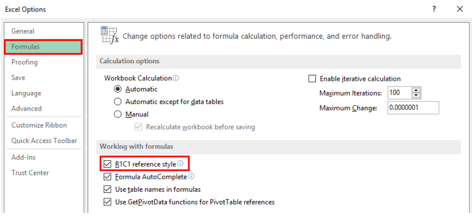 Figure 3. Check R1C1 reference style
The column labels will automatically change from letters to numbers.
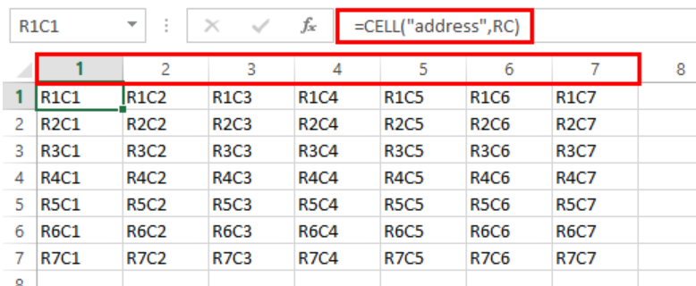 Figure 4. Columns are numbers in R1C1 style
The cell address will also change from A1 to R1C1. The R1C1 reference style is easier to understand because it gives both the row number and column number of a cell. R refers to row while C refers to column. R1C1 means row 1 and column 1, while R7C7 refers to the cell in row 7 column 7.
Note that R1C1 format does not change the formulas in our cells. Only the format of referencing cells is changed.
How to number columns
Most of us are not used to the R1C1 reference style. If we only want to number columns but keep the column labels as letters, we can simply insert numbers on the first row of our worksheet.
- Uncheck the R1C1 reference style check box in Excel Options > Formulas to revert back to A1 style
- In cell A1, enter the value “1”
- In cell B1, enter the value “2”
- Select cells A1 and B1
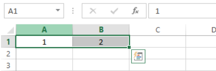 Figure 5. Select the cells and click the fill handle
- Click the Fill Handle, which appears as a plus “+” sign when we hover the cursor over the bottom right corner of cell B2
- Drag the fill handle to the right up to column G.
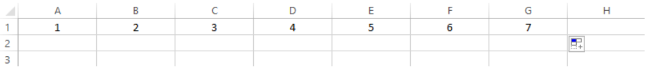 Figure 6. Output: How to number columns
We have successfully inserted column numbers at the top row of our worksheet.
Instant Connection to an Excel Expert
Most of the time, the problem you will need to solve will be more complex than a simple application of a formula or function. If you want to save hours of research and frustration, try our live Excelchat service! Our Excel Experts are available 24/7 to answer any Excel question you may have. We guarantee a connection within 30 seconds and a customized solution within 20 minutes.