
If you have a worksheet with data in columns that you need to rotate to rearrange it in rows, use the Transpose feature. With it, you can quickly switch data from columns to rows, or vice versa.
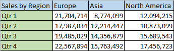
For example, if your data looks like this, with Sales Regions in the column headings and and Quarters along the left side:
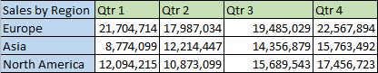
The Transpose feature will rearrange the table such that the Quarters are showing in the column headings and the Sales Regions can be seen on the left, like this:
Note: If your data is in an Excel table, the Transpose feature won’t be available. You can convert the table to a range first, or you can use the TRANSPOSE function to rotate the rows and columns.
Here’s how to do it:
-
Select the range of data you want to rearrange, including any row or column labels, and press Ctrl+C.
Note: Ensure that you copy the data to do this, since using the Cut command or Ctrl+X won’t work.
-
Choose a new location in the worksheet where you want to paste the transposed table, ensuring that there is plenty of room to paste your data. The new table that you paste there will entirely overwrite any data / formatting that’s already there.
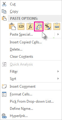
Right-click over the top-left cell of where you want to paste the transposed table, then choose Transpose
 .
.
-
After rotating the data successfully, you can delete the original table and the data in the new table will remain intact.
 .
.
Tips for transposing your data
-
If your data includes formulas, Excel automatically updates them to match the new placement. Verify these formulas use absolute references—if they don’t, you can switch between relative, absolute, and mixed references before you rotate the data.
-
If you want to rotate your data frequently to view it from different angles, consider creating a PivotTable so that you can quickly pivot your data by dragging fields from the Rows area to the Columns area (or vice versa) in the PivotTable Field List.
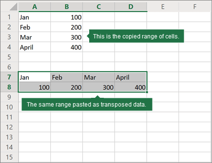
You can paste data as transposed data within your workbook. Transpose reorients the content of copied cells when pasting. Data in rows is pasted into columns and vice versa.
Here’s how you can transpose cell content:
-
Copy the cell range.
-
Select the empty cells where you want to paste the transposed data.
-
On the Home tab, click the Paste icon, and select Paste Transpose.
Excel 2021 Excel 2019 Excel 2016 Excel 2013 Office for business Excel 2010 More…Less
Summary
When you use the Microsoft Excel products listed at the bottom of this article, you can use a worksheet formula to covert data that spans multiple rows and columns to a database format (columnar).
More Information
The following example converts every four rows of data in a column to four columns of data in a single row (similar to a database field and record layout). This is a similar scenario as that which you experience when you open a worksheet or text file that contains data in a mailing label format.
Example
-
In a new worksheet, type the following data:
A1: Smith, John
A2: 111 Pine St.
A3: San Diego, CA
A4: (555) 128-549
A5: Jones, Sue
A6: 222 Oak Ln.
A7: New York, NY
A8: (555) 238-1845
A9: Anderson, Tom
A10: 333 Cherry Ave.
A11: Chicago, IL
A12: (555) 581-4914 -
Type the following formula in cell C1:
=OFFSET($A$1,(ROW()-1)*4+INT((COLUMN()-3)),MOD(COLUMN()-3,1))
-
Fill this formula across to column F, and then down to row 3.
-
Adjust the column sizes as necessary. Note that the data is now displayed in cells C1 through F3 as follows:
Smith, John
111 Pine St.
San Diego, CA
(555) 128-549
Jones, Sue
222 Oak Ln.
New York, NY
(555) 238-1845
Anderson, Tom
333 Cherry Ave.
Chicago, IL
(555) 581-4914
The formula can be interpreted as
OFFSET($A$1,(ROW()-f_row)*rows_in_set+INT((COLUMN()-f_col)/col_in_set), MOD(COLUMN()-f_col,col_in_set))
where:
-
f_row = row number of this offset formula
-
f_col = column number of this offset formula
-
rows_in_set = number of rows that make one record of data
-
col_in_set = number of columns of data
Need more help?
Excel Columns to Rows (Table of Contents)
- Columns to Rows in Excel
- How to Convert Columns to Rows in Excel using Transpose?
Columns to Rows in Excel
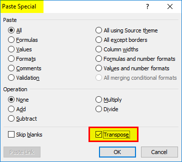
In Excel, to convert any Columns to Rows, first select the column which you want to switch and copy the selected cells or columns. To proceed further, go to the cell where you want to paste the data. Then from the Paste option, which is under the Home menu tab, select the Transpose option. This will convert the selected Columns into Rows. You can also use the shortcut keys Alt + H + V + T, which will directly take us to the TRANSPOSE function.
Paste Special Option.
The shortcut key for paste special:
Once you have copied the range of cells that need to be transposed, click on Alt + E + S in a cell where you want to paste special a dialog box popup window with the transpose option.
How to Convert Columns to Rows in Excel using Transpose?
Converting data from column to row in excel is very simple and easy. Let’s understand the working of converting columns to rows by using some examples.
You can download this Convert Columns to Rows Excel Template here – Convert Columns to Rows Excel Template
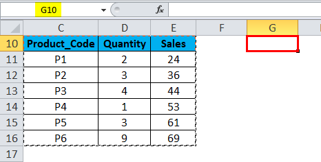
Example #1
The below-mentioned Pharma sales table contains the medicine product code in column C (C10 to C16), quantity sold in column D (D10 to D16) & total sales value in column E (E10 to E16).
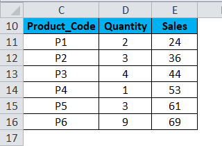
Here we need to convert its orientation from columns to rows with the help of a paste special option in excel.
- Select the whole table range, i.e. all the cells with the dataset in a spreadsheet.
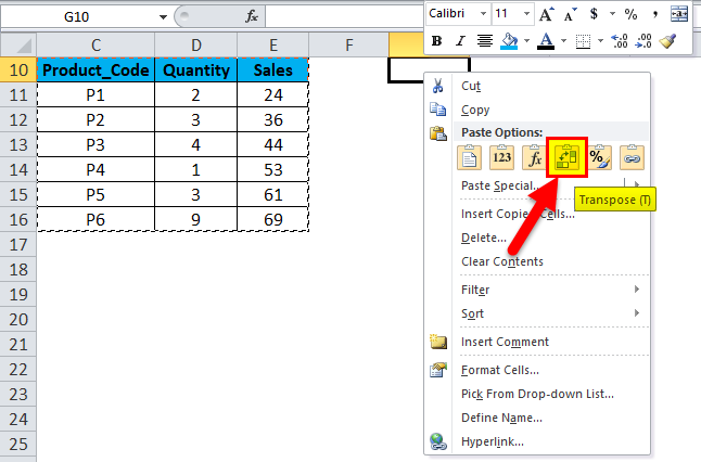
- Copy the selected cells by pressing Ctrl + C.
- Select the cell where you want to paste this data set, i.e. G10.
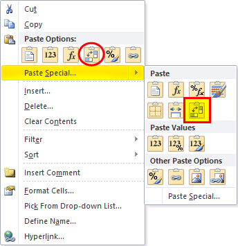
- When you enable right-click on the mouse, the paste option appears. You must then select the 4th option, i.e. Transpose (As mentioned in the below screenshot)
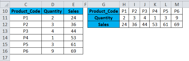
- On selecting the transpose option, your dataset gets copied in that cell range starting from cell G10 to M112.
- Apart from the above procedure, you can also use a shortcut key to convert columns to rows in excel.
- Copy the selected cells by pressing Ctrl + C.
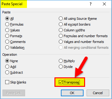
- Select the cell where you need to copy this data set, i.e. G10.
- Click on Alt + E + S, paste special dialog box popup window appears, in that select or click on the box of Transpose option, it will result or convert column data to rows data in excel.
Data that is copied is called source data, and when this source data is copied to other ranges, i.e. pasted data, which is referred to as transposed data.
Note: In the other direction where you are going to copy raw or source data, you have to ensure to select the same number of cells as the original set of cells so that there is no overlapping with the original dataset. In the above-mentioned example, there are 7-row cells that are arranged vertically. So when we copy this dataset to the horizontal direction, it should contain 7 column cells towards the other direction so that the overlapping does not occur with the original dataset.
Example #2
Sometimes, when you have huge number of columns, column data at the end is not visible, and it does not fit to screen. In this scenario, you can change its orientation from the current horizontal range to the vertical range with the help of the paste special option in excel.
- The table contains months and their serial number (From columns C to W).
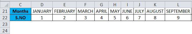
- Select the whole table range, i.e. all the cells with the dataset in a spreadsheet.
- Copy the selected cells by pressing Ctrl + C.
- Select the cell where you need to copy this data set, i.e. C24.
- When you right-click on the mouse, the paste options appear, in that you have to select 4th option, i.e. Transpose (Below mentioned screenshot)
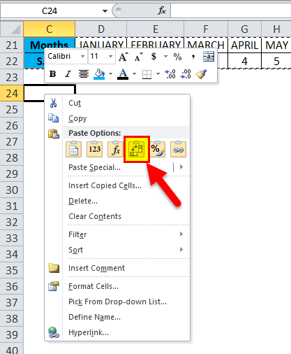
- On selecting the transpose option, your dataset gets copied in that cell range starting from cell C24.
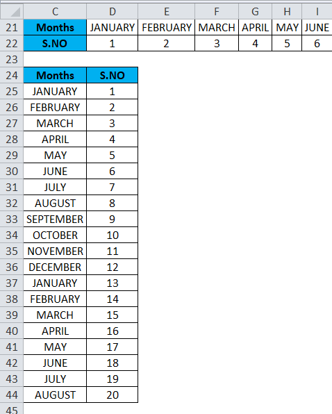
In the transposed data, all the data values are visible and clear as compared to the source data.
Disadvantages of using Paste special option:
- Sometimes copy-paste option creates duplicates.
- If you have used the Paste special option in excel to convert columns to rows, the transposed cells (or arrays) are not linked to each other with source data, and it does not get updated when you try to change data values in source data.
Example #3
Transpose function: It converts columns to rows and rows to columns in excel.
The syntax or formula for the Transpose function is:
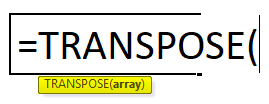
- Array: It is a range of cells that you need to convert or change their orientation.
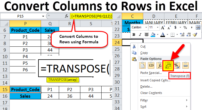
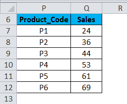
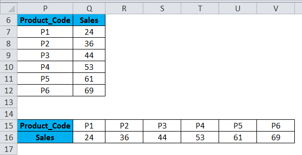
In the below example, the Pharma sales table contains medicine product code in column P (P7 to P12), and sales data in column Q (Q7 to Q12).
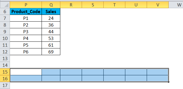
Check out the number of rows & columns in the source data which you want to transpose.
i.e. Initially, count the number of rows and columns in your original source data (7 rows & 2 columns) which is vertically positioned. Now select the same number of blank cells, but in the other direction (Horizontal), i.e. (2 rows & 7 columns)
- Prior to entering the formula, select the empty cells, i.e. from P15 to V16.
- With the empty cells selected, Type the transpose formula in cell P15. i.e. = TRANSPOSE (P6:Q12).
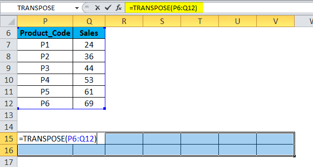
- Since the formula needs to be applied for the whole range, press Ctrl + Shift + Enter to make it an array formula.
Now you can check the dataset; here, columns are converted to rows with datasets.
Advantages of the TRANSPOSE function:
- The main benefit or advantage of using the TRANSPOSE function is that transposed data or the rotated table retains the connection with the source table data, and whenever you change the source data, the transposed data also changes accordingly.
Things to Remember about Convert Columns to Rows in Excel
- Paste special option can also be used for other tasks, i.e. Add, Subtract, Multiply, and Divide between datasets.
- #VALUE error occurs while selecting the cells, i.e. If the number of columns and rows selected in transposed data are not equal to the rows and columns of the source data.
Recommended Articles
This has been a guide to Columns to Rows in Excel. Here we have discussed how to convert columns to rows in excel using transpose along with practical examples and a downloadable excel template. Transpose can help everyone to convert multiple Columns to Rows in excel easily and quickly. You can also go through our other suggested articles –
- COLUMNS Formula in Excel
- Add Rows in Excel Shortcut
- Column Header in Excel
- VBA Columns
In Excel one can easily convert data columns to rows or multiple data rows to columns which is technically named transpose.
What is Transpose?
In Excel switching or rotating columns to rows or rows to columns is called Transposing the data.
And this actually shifts the dimensions of data and along with it definitely the address of different data bits will also change. Therefore, if you are into transposing your data, do it with caution as if you shift the data the dependent cells might miscalculate the figures.
Love reading about Excel? Subscribe my youtube channel dedicated to Excel.
[vc_btn title=”Subscribe” style=”custom” custom_background=”#ff0000″ custom_text=”#ffffff” size=”lg” align=”right” i_icon_fontawesome=”fa fa-youtube-play” add_icon=”true” link=”url:https%3A%2F%2Fgoo.gl%2Fx16inH||target:%20_blank|”]
Many already know how to do this. But for those who don’t this one minute Excel tutorial is for them. By the way, yes! you can use pivot tables to shift rows as columns. To learn how to make pivot tables read this readers’ favourite tutorial. And most probably you will figure out the way how rows are shifted as columns using pivot tables.
We have several ways to switch or rotate Excel data columns to rows or vice versa to accomplish this task. Following are the transpose methods we are discussing today in which few involve converting columns to rows using Excel formulas:
- Use Paste Special
- Use TRANSPOSE function
- Use INDIRECT function
- Use INDEX function
- Use Paste Special + Common Sense
Method 1: Convert columns to rows using Paste Special
Copying and Pasting is one great thing happened to PC. With Paste Special it really went miles ahead. In Excel you can copy a data and then using paste special functionality you can twist, rotate, manipulate, process and do other things with the data very easily including Transpose i.e. flipping columns to rows or rows to columns. To do this following steps will help:
Step 1: Select the data that you want to transpose and copy it using the copy button or with Ctrl+C shortcut.
Step 2: Go to the cell where you want the data to paste. And go to Home tab > clip board group > click the drop down button just under paste button > select:
- under paste sub-group click transpose button that comes with this icon; OR
- Select paste special. This will open the paste special dialogue from which check the transpose checkbox and click OK button
Your data will be transposed instantly. Told ya! it is easy!
Method 2: TRANSPOSE Function to switch columns to rows or vice versa
Yes there is a function that can do the somersault called TRANSPOSE. The use of this function is a little tricky and requires knowing more than pressing TAB so follow the steps closely.
IMPORTANT: Determine the rows and columns of your data. For example you have 2 columns and 7 rows. Once you transpose the data it will be 2 rows and 7 columns.
Step 1: Determine the rows and columns of data. In our case it is 7 rows and 2 columns
Step 2: Select a vacant region in the worksheet which is 2 rows deep and 7 columns wide.
Step 3: Press F2 key to enter edit mode while the region still selected.
Step 4: Write TRANSPOSE function following the equal sign and enter the data range that you want to transpose
Step 5: Hit CTRL+SHIFT+ENTER. Yes! Not just Enter key but Ctrl+Shift+Enter as this is an array formula
TANGO! Your data is transposed!
Benefit of TRANSPOSE Function
The best thing with using TRANSPOSE function is that if you change the values in the source range then transposed range will also change accordingly. So basically it is a live-transposed-range of the source-range.
But as this is an array function this is very much dependent on the source and if you try to change anything this tends to break. Therefore, even if it is good for many reasons, it is hard go by in many situations. So follow along to learn some more easier to go tricks to get the data transposed in Excel.
Method 3: TRANSPOSE Using INDIRECT function
INDIRECT function was introduced in one of my favourite article some time back in which we learned how to build a reference to worksheet based on cell value. I must confess that I used to think INDIRECT has very little use but this little function can prove tremendous help.
Today we will look at another use of INDIRECT function i.e. to transpose the data. However, if you use this function the treatment for column to row shift is a little different from row to column shift. So I will explain both one by one.
Transpose – Column to Row using INDIRECT
Suppose our data is based on 2 columns A and B and 7 rows from 1 to 7.
The data of column A has address like A1, A2, A3,…. A7. In this A is constant whereas due to additional rows we have increasing numbers from 1 to 7. If you understand up to this, you will understand what we are about to learn.
Lets say you want to put the transposed data starting at cell C10. I will put this formula in cell C10 and press Enter key:
=INDIRECT(“A”&COLUMN()-2)
And this formula in C11 and press Enter:
=INDIRECT(“B”&COLUMN()-2)
Now select these two cells and drag the fill handle across to column I. So there you have the data transposed. But lets understand what formula is actually doing.
Understanding INDIRECT approach to TRANSPOSE
As told earlier Indirect formula helps in converting text strings to cell references. COLUMN function actually gives us the number of column in which the formula is entered. For example if you put =COLUMN in any cell of column A it will give the value of 1 as it is first column. Similarly if you put the COLUMN function in any cell of column I, it will return 9 as it is 9th column.
So with the column function we were able to incremental numbers as we drag the formula across columns. But as we inserted the formula in third column and the not first column so it would have returned 3 in which case the first address to be fetched would have been A3. But we want the values from first cell of column A therefore we had to insert “-2”. This way we got 1, 2, 3 and not 3, 4, 5
So the formula: =INDIRECT(“A”&COLUMN()-2)
In the above formula “A” is provided as text string which is joined (concatenated) using “&” with the values generated through COLUMN function. And thus successfully built the cell references.
Now if you change the values in source range the transposed range will also change. But it is much more flexible as it won’t break if you change one item in transposed range manually.
Transpose – Rows to Columns using INDIRECT
Using the same technique learnt above, we can transpose the data from rows to columns. But in this case you will use ROWS() function instead of COLUMNS to work correctly.
As you are converting rows to columns therefore you will be going down the rows and thus you require number increments as rows are jumped. So simply adjust the formula as per your needs and use ROW instead of COLUMN and it will do the rest for you.
No you can’t simply replace the COLUMN function with ROW function as mentioned above to convert the rows back to columns. Instead you will have to use the combination of INDIRECT, ADDRESS and ROW function.
In my case to transpose first row to column I used the formula: =INDIRECT(ADDRESS(10,ROW()-11))
Whereas to convert the second row to column I used this formula: =INDIRECT(ADDRESS(11,ROW()-11))

Method 4: TRANSPOSE using INDEX functions
Using the technique learnt to transpose columns to rows above. You can use INDEX function if building reference is difficult for you and you still have your head spinning.
INDEX function is one great addition to Excel functions and formulas repository. Lets have a look at the syntax of INDEX very briefly so that we understand how can we use it to transpose the data.
INDEX(array, row_num, [column_num])
array: the range, in our case it is the range we want to transpose
row_num: the row number. In this function we have mention row number to help it fetch the value
[column_num]: this is the optional argument. If not mentioned the column number doesn’t change and it will be the same in which function is applied. But today we need this option badly!
Transposing Rows to Columns using INDEX function
Suppose our data is arranged from cell A1 to G2. Two rows and seven columns in other words. So if we transpose the data we will have 2 columns and 7 rows.
To transpose the data arranged in a row to column go to the cell from where you want the data to start. I selected cell C6 and D6 and put theses formula:
Cell C6: =INDEX($A$1:$G$2,1,ROW()-5)
Cell D6: =INDEX($A$1:$G$2,2,ROW()-5)
Select both cells and drag the fill handle down to next six rows i.e. row 12. And you will get the data transposed from rows to columns.
Understanding the formula
Lets take some time to understand the mechanics of this formula. The formula we applied in cell C6 is as follows:
=INDEX($A$1:$G$2,1,ROW()-5)
array: [$A$1:$G$2] – this is the range that we want to transpose. The reference is made absolute so that as we drag the formula this array stays static and does not change.
row_num: [1] – this represent the first row of the data and we mentioned it so that INDEX function recognize that we want it to fetch the values only from row 1 of selected array i.e. $A$1:$G$2.
column_num: [ROW()-5] – Our data A, B, C, … G is in one row but across 7 columns. That means the address of:
- value A is first row-first column
- value B is first row-second column
- value C is first row-third column; and so on…
So as we drag the formula down, we want the formula to get the values from 1st, 2nd, 3rd, 4th, 5th, 6th and 7th column. To do this we have to tell the column number. Now one way is to mention column number manually every time we put the INDEX function in next cell so that it fetches the right value.
But to automate the process of feeding column numbers to the function, I used ROW() function as the argument of column number (column_num). And as I drag the fill handle down, the ROW function will churn out row numbers inside the formula.
ROW function gives the row number. Now as I have put the INDEX function cell C6 the ROW function will tell that ROW number is 6. But we want it to be 1 as I want to fetch the values from the first column of the selected array. That is the reason we have “-5” following ROW() inside the formula. So it reduces the numbers generated by ROW function by 5 and this it will give 1, 2, 3, … 7.
Transposing Columns to Rows using INDEX function
Once you understand how INDEX function has fetched the values in above situation. Its easy to understand how to tackle the data which is arranged in columnar form and we want it to shift in rows.
For this we will make two changes:
for row_num: now we will use COLUMN() function generate numbers so that as we drag the formula towards right the row number will get updated because we are jumping across columns and thus COLUMN function will fetch the column number. Adjust the value generated by column number by adding or subtracting constants so that you get the desired result.
for column_num: mention 1 or 2 depending on the column within the selected array from which you want the values fetched.
Example
For example my data is based in 2 columns 7 rows and is housed in column C and D starting at Row 6.
I want the data transposed in rows 13 and 14 in column F. Therefore I put these formula:
cell F13:
=INDEX($C$6:$D$12,COLUMN()-5,1)
cell F14:
=INDEX($C$6:$D$12,COLUMN()-5,2)
Select both cells and drag to the right until column L
Method 5: Paste Special + Common Sense = Paste Ultimate!
We saw TRANSPOSE function went ahead of Paste Special as it was not only able push columns as rows (transpose) but were also live as transposed range was able to update as source change. We fixed some of the TRANSPOSE nuisances through INDIRECT approach. But writing formula and then dragging the range takes time.
But can we get TRANSPOSE like result using paste special? The answer is yes!
Paste Link
To get the live feed of source range we can use Paste Special’s inhouse capability called Paste link. Paste link pastes the cell references and not the values in cell and if source data changes, the linked cell will also change.
However, for unknown reasons, if you try to transpose and paste link at the same time Excel does not allow that i.e. you can either transpose or paste link. In other words, if you click Paste Link button with transpose option checked, the moment you select transpose option the paste link button gets disabled.
To get around this misery we took help of our Agent-X named common sense. Follow along!
Step 1: Copy the range and go to any vacant space in the same worksheet.
Step 2: Hit Alt+Ctrl+V to invoke paste special dialogue box and hit the button paste link. This will paste NOT the cell values but the cell references of the range you copied.
Step 3: Select the range you just pasted and hit Ctrl+H. This will bring up the REPLACE dialogue.
Step 4: In ‘Find what’ field mention equal sign i.e. “=” (without quotes) and in replace with field mention “HS=” and hit Replace ALL button. This will actually convert the formula into text as you have just replaced the equal sign with HS=
Step 5: Copy the range again and now go to the place where you want to put the transposed range. Hit Alt+Ctrl+V to bring the paste special dialogue box. Select the Transpose option and click OK. This will effectively transpose the data.
Step 6: To revert the formulas back in place so that you get the correct values in place from the source range. Hit Ctrl+H again. This time in Find what field put HS= and in replace with mention =. Hit Replace ALL button.
Now you have the live-transposed-range of the source WITHOUT using TRANSPOSE function or similar alternatives. How cheeky was that! 😉
So how do you do the transpose? If you have new ideas or any better versions of the ideas discussed do let me know in the comment section
How to Convert Rows to Columns in Excel?
There are two different methods for converting rows to columns in Excel, which are as follows:
- Method #1 – Transposing Rows to Columns Using Paste Special.
- Method #2 – Transposing Rows to Columns Using TRANSPOSE Formula.
Table of contents
- How to Convert Rows to Columns in Excel?
- #1 Using Paste Special
- Example
- #2 Using TRANSPOSE Formula
- Example
- Advantages
- Disadvantages
- Things to Remember
- Recommended Articles
- #1 Using Paste Special
#1 Using Paste Special
It is an efficient method; it is easy to implement and saves time. Also, this method would be ideal if you want your original formatting to be copied.
You can download this Convert Rows to Columns Excel Template here – Convert Rows to Columns Excel Template
Example
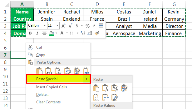
For example, if you have below data of key industry players from various regions, it also shows their job roles as shown in figure1.
| Name | Jennifer | Racheal | Milos | Costas | Daniel | Kevin |
| Country | Spain | England | France | Brazil | Ireland | Germany |
| Job Role | CTO | CEO | Analyst | Analyst | Media | Director |
| Domain | Electronics | Chemical | Mechanical | Aerospace | Marketing | Finance |
In example 1, the players’ names are written in column form. Still, the list becomes too long, and the data entered also seems unorganized. Hence, we would change the rows to columns using paste special methodsPaste special in Excel allows you to paste partial aspects of the data copied. There are several ways to paste special in Excel, including right-clicking on the target cell and selecting paste special, or using a shortcut such as CTRL+ALT+V or ALT+E+S.read more.
The steps to convert rows to columns in Excel using the Paste Special method are as follows:
- Select the whole data which needs to be transformed or transposed. Then, Copy the selected data by simply pressing Ctrl + C keys.

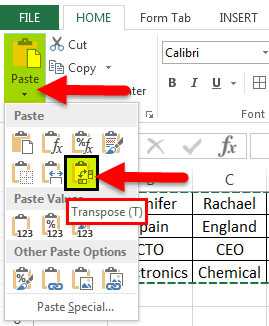
- Select a blank cell and ensure it is outside the original data range. Paste the data by pressing the “Ctrl +V” keys starting at the first blank space or cell. Then, select the down arrow from the toolbar under the “Paste” option and select “Paste Transpose.” But the easy way is to right-click the blank you chose first to paste the data. Then, select “Paste Special” from it.

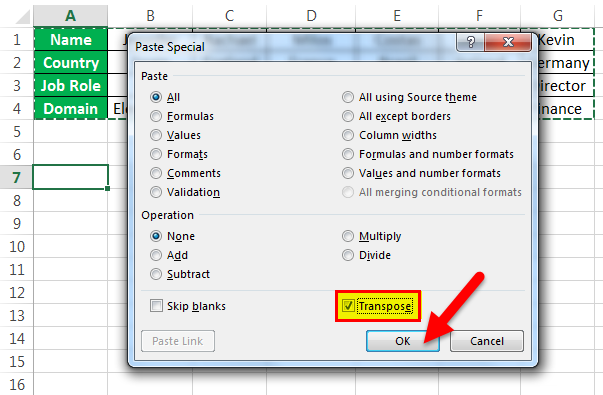
- Then, a “Paste Special” dialog box will appear from which select the “Transpose” option. And click “OK.”

- In the above figure, copy the data which needs to be transposed and then click on the down arrow of the Paste option and form the options select Transpose. (Paste-Transpose)

It shows how the transpose function is performed to convert rows to columns.


#2 Using TRANSPOSE Formula
When a user wants to keep the same connections of the rotating table with the original table, it can use a transposing method using a formula. This method is also quicker in converting rows to columns in Excel. But, it does not keep the source formatting and links it to a transposed table.
Example
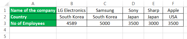
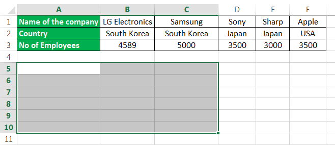
Consider the example below, as shown in figure 6, where it shows the company’s names, location, and the number of employees.
The steps to transpose rows to columns in excel using formula are as follows:
- First, count the number of rows and columns in your original excel table. And then, select the same number of blank cells but ensure you have to transpose the rows to columns to choose the blank cells in the opposite direction. Like in example 2, the number of rows is 3, and the number of columns is 6. So, you will select 6 blank rows and 3 blank columns.
- In the first empty cell, enter the TRANSPOSE formula in excelThe TRANSPOSE function in excel helps rotate (switch) the values from rows to columns and vice versa. Being a part of the Excel lookup and reference functions, its purpose is to organize the data in the desired format. To execute the formula, the exact size of the range to be transposed is selected and the CSE key (“Control+Shift+Enter”) is pressed.
read more ‘=TRANSPOSE($A$1:$F$3)’.
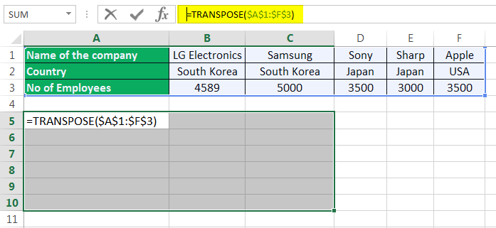
- Since this formula needs to be applied for other blank cells so press ‘Ctrl+Shift+Enter.’
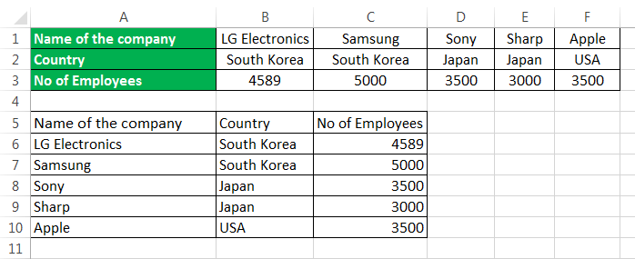
The rows are converted to columns.
Advantages
- The Paste Special method is useful when the user needs the original formatting to be continued.
- In the transpose method, by using the TRANSPOSE function, the converted table will change its data automatically, which means that whenever the user changes the data in the original table, it will automatically change the data in the transposed table, as it is linked to it.
- Converting the rows to columns in Excel sometimes helps the user to make the audience understand their data easily and so that the audience interprets it without much effort.
Disadvantages
- If the number of rows and columns increases, then the transpose method using the Paste Special options cannot perform efficiently. In this case, the “TRANSPOSE” function will be disabled when there are many rows to be converted to columns.
- The “Transpose Paste Special” option does not link the original data to the transposed data. Therefore, if you need to change the data, you must repeat all the steps.
- In the transpose method, the source formatting is not kept the same for the transposed data by using the formula.
- After converting the rows to columns in Excel using a formula, the user cannot edit the data in the transposed table as it is linked to the source data.
Things to Remember
- We can transpose rows to columns using Paste Special methods. We can link the data to the original data by selecting “Paste Link” from the “Paste Special” dialog box.
- We can also use Excel’s INDIRECT formula and ADDRESS functions in ExcelThe address function finds the cell’s address and returns an absolute value. It requires two mandatory arguments: the row number and the column number. For example, if we use =Address(1,2), the result will be $B$1.read more to convert rows to columns and vice-versa.
Recommended Articles
This article is a guide to Convert Rows to Columns in Excel. Here, we discuss switching rows to columns in Excel using the Paste Special and TRANSPOSE formula, practical examples, and a downloadable Excel template. You may learn more about Excel from the following articles: –
- Group Columns in ExcelIn Excel, grouping one or more columns together in a worksheet is referred to as group column and I t allows you to contract or expand the column.read more
- Compare Two Columns in ExcelTwo columns in excel are compared when their entries are studied for similarities and differences.read more
- Use Columns Formula in Excel
- Column Sort in Excel