
I’m using Office 2013 on Windows 7. Few times, I have not been able to insert rows / columns in a some of the Excel spreadsheets. I tried the following before searching on the internet.
- Use right-click on the column border to select «Insert» option — the
option is not grayed out — but it does no action — no rows/columns inserted - Click on the «Insert» icon (which is under the «Cells» group of the
«Home» tab) — select the «Insert sheet rows / Insert sheet columns»
option from the sub-menu — nothing happens - Tried using a keyboard shortcut
Ctrl+Shift++ to add rows / columns
after selecting a particular column or row — no rows/columns
inserted.
When I googled, I found lot of search results pointing to the error What does ‘To prevent possible loss of data, Excel cannot shift nonblank cells off of the worksheet» mean? But I’m not getting any such error message when I attempt the insertion of row / column.
There are no patterns of files for which this row/column insert operation fails. Sometimes, it happens to a file on a network server or sometimes to the files on my PC.
The present workaround is to restart Excel and most times it allows row/column insertion on the same file. Has anyone come across similar issues? Any fixes found so far?
asked Nov 10, 2014 at 18:52
![]()
6
I am using Office 2013 Pro Plus and I have also lost my «Insert» option and even «Cut» option along with that.
To overcome that, go to following file path:
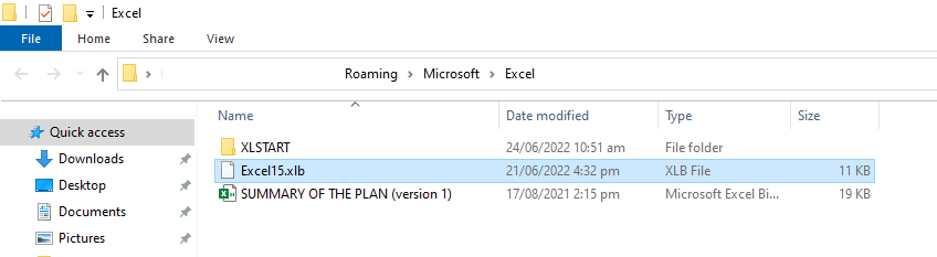
C:Users(user ID)AppDataRoamingMicrosoftExcelExcel15.xlb
rename Excel15.xlb file to Excel15.db.
P.S : Keep Excel off while change.
![]()
techraf
4,83211 gold badges24 silver badges40 bronze badges
answered Aug 31, 2015 at 7:45
![]()
RahulRahul
511 bronze badge
4
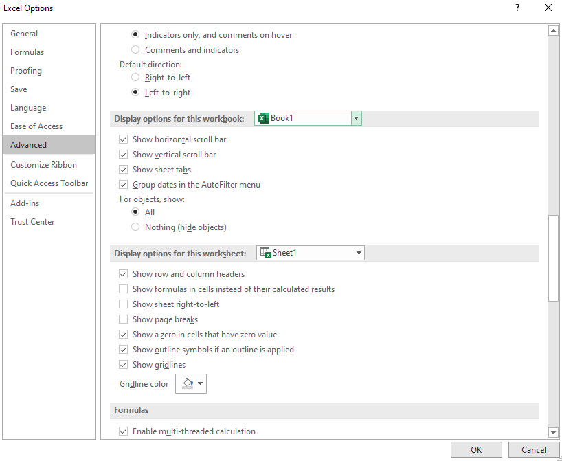
The «Cannot shift objects off worksheet» message occurs when you attempt to insert rows or columns in a worksheet, and the option Nothing (hide objects) is selected under the For objects, show section in the Excel Options dialog box. This is a known bug in Microsoft Office Excel 2007. Although this option is not selected by default, it’s possible to set it accidentally by pressing a particular keyboard shortcut (CTRL+6).
To work around the bug, you must change the setting from Nothing (hide objects) to All. The fastest way to do this is by pressing CTRL+6.
Alternatively, you can change the setting in the Excel Options dialog box. To do so, click the Microsoft Office Button , and then click Excel Options. On the Advanced tab, scroll to Display options for this workbook settings. Under For objects, show, select All instead of Nothing (hide objects).
answered Feb 5, 2015 at 7:04
![]()
2
MS Excel -2013 — Adding a Column or Row — Problem
- File-> Options
- Click on ‘Customize Ribbon’
- Click ‘New Tab’, Rename if you want, Say ‘X’. Click ‘Insert Sheet
Columns’. This action will add this to ‘New Tab’ created. - Click ‘Insert Sheet Rows’. This action will add this to ‘New Tab’
created. - Click ‘Close’.
- Select any Column.
- You will see a new tab, ‘X’.
- Click on ‘Insert Sheet Columns’, from the new tab ‘X’.
This will Add a Ribbon on the top to help you in inserting a row or column, alternate to Right click to add a row or column. Not fixing the issue. Just a workaround.
![]()
answered Aug 20, 2015 at 6:09
![]()
2
Contents
- Why Can’t I Create New Cells in Excel on Windows 10?
- Any of the following factors can prevent the creation of new cells in Microsoft Excel:
- How to Fix “Cannot Add New Cells in Excel”
- Here are the solutions to the problem:
- Fix 1: Remove Cell Protection
- Fix 2: Unmerge the Rows/Columns
- Fix 3: Unfreeze the Panes
- Fix 4: Copy Your Data to a New Sheet
- Fix 5: Choose a Shorter File Path
- Fix 6: Change the File Format
- Fix 7: Format the Table as a Range
- Fix 8: Set the File Source as Trusted
- Fix 9: Clear the Formatting in Unused Rows/Columns
- Fix 10: Customize the Used Range Using VBA
- Fix 11: Use Office Online
![Microsoft Excel cannot add new cells [Fixed]](https://www.auslogics.com/en/articles/wp-content/uploads/2020/07/fix-excel-cant-add-new-cells.jpg)
While working on an Excel spreadsheet, you may run into the problem of not being able to add new cells. This issue is very common and can be easily resolved. Keep reading to find out how.
Why Can’t I Create New Cells in Excel on Windows 10?
In most cases, the supposed ‘problem’ serves the purpose of preventing the loss of data on your sheet. However, exceptions do exist, such as in the case of corrupt files or due to the file format you are using.
Any of the following factors can prevent the creation of new cells in Microsoft Excel:
- Cell protection: In Excel, there are different types of cell protection for your data. If you have one active, it could be the reason why you cannot create a new cell.
- Merged rows/columns: When you merge entire rows or columns to make a single cell, you won’t be able to insert a new row/column.
- Formatting applied to an entire row/column: You may have unintentionally formatted an entire row/column. This could be the cause of the problem you are facing.
- Freeze Panes: The Freeze Panes option helps facilitate data entry and management. However, it can prevent you from adding new cells.
- Entries in the last rows/columns: If you are trying to replace entries in the last row/column of the sheet, Excel will restrict the addition of new cells so as to avoid data loss.
- A data range formatted as a table: You may experience the problem in question when you try to add cells in a selected area that includes a table and a blank space.
- File format limitations: Different file formats are available in different versions of Excel. Each file format has its unique purpose and limitations. You may thus encounter a problem when trying to add new cells if you are using a file format with limited functionality.
- Files from untrusted sources: For your protection, Excel often prevents the execution of files from untrusted sources. It may well be that the error you are currently facing stems from the file itself.
Now that we have seen the various reasons why you can’t add a column or line in Microsoft Excel, let us now go ahead and dive into how to get the issue resolved.
How to Fix “Cannot Add New Cells in Excel”
Here are the solutions to the problem:
- Remove cell protection
- Unmerge the rows/columns
- Unfreeze the panes
- Copy your data to a new sheet
- Choose a shorter file path
- Change the file format
- Format the table as a range
- Set the file source as trusted
- Clear the formatting in unused rows/columns
- Customize the used range using VBA
- Use Office Online
By the time you have tried the solutions listed above, you are sure to get on with your work without further trouble. So let’s get started:
Fix 1: Remove Cell Protection
The cell protection functionality in Excel preserves the current state of your sheet or workbook by locking the cells so that your data can’t be wiped or edited. Therefore, if you have cell protection active, the creation of new cells will not be allowed in order to preserve your existing data. So all you have to do is deactivate the functionality. Follow these easy steps to get it done:
- Select all the cells on your worksheet by pressing Ctrl + A on your keyboard.
- On the Home tab, click the Format drop-down.
- Select Format Cells under Protection at the bottom of the menu.
- In the window that opens, click on the Protection tab and unmark the option that says ‘Locked.’
- Click OK.
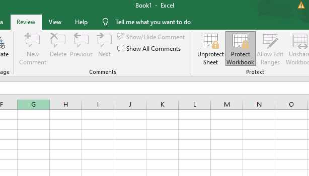
- Now, go to the Review tab and click on Protect workbook or Protect Sheet.
- Enter your password to remove protection from the sheet or workbook.
- Press Ctrl + S to save your file. Close the window and then open it again. You can now try inserting a new row/column. See if it works.
Fix 2: Unmerge the Rows/Columns
As already mentioned, you may have merged an entire row or column rather than just a few cells. In this case, Excel is programmed to restrict the addition of new cells so as to keep your data from getting lost. Merging all the cells in a row prevents the addition of another column, and merging all the cells in a column prevents the addition of new rows. Unmerging the columns/rows can resolve the issue. Here’s what you should do:
- Look through your worksheet and locate the merged rows/columns.
- If it is a column that is merged, click the column header (for example A, B, C, etc.).
- Now, on the Home tab, click on Merge and Center to unmerge the highlighted column.
- Repeat Steps 2 and 3 for any other merged column(s).
- If there is any merged row, click on the row header (for example 1, 2, 3, etc.) and then click Merge and Center displayed in the Home tab.
- Press Ctrl + S on your keyboard to save your file. Close the workbook and then open it again. You can now check whether the issue in question has been resolved.
Fix 3: Unfreeze the Panes
The Freeze Panes feature makes referencing easier by keeping a selected area of your worksheet visible as you scroll to other areas of the worksheet. However, the functionality can prevent the addition of new rows or columns to the sheet. Follow these steps to unfreeze the frozen panes:
- Go to the View tab.
- Click the Freeze Panes drop-down.
- Select Unfreeze Panes from the menu.
- Save your file by pressing Ctrl + S and then close it.
- Reopen the file and see if the problem has been fixed.
Fix 4: Copy Your Data to a New Sheet
It could well be that the file you are working with is corrupt. Thus, try copying your data to a new file. Here’s how:
- Open the sheet you are having problems with.
- Press Ctrl + A to select your data and then press Ctrl + C to copy it.
- Go to the File tab.
- Click on New and select Blank Workbook.
- Click Create.
- Click the Paste drop-down arrow in the Home tab.
- Click ‘Paste Special…’
- Click on ‘Values’ and then click OK.
- Save the new file and then close it. Reopen the file and check whether the problem you are facing has been resolved.
Fix 5: Choose a Shorter File Path
The address of your file in your OS is referred to as the file’s path. When it is too long, it could prevent the creation of new cells. Save the file in a location where the file path will be shorter. Follow these steps:
- Open the file you are having trouble with.
- Click on the File tab and select Save as.
- In the dialogue box that opens, select Desktop as the location for the file to be saved and then click the Save button.
- Close the workbook.
- Open the newly saved file and check whether the problem you were facing will occur again.
Fix 6: Change the File Format
The file format you are using may be the cause of the error. Using a different format may help resolve the issue. For instance, you can switch from XLSM to CSV, XLS, or XLSX. Let’s take a look at how to do that:
- Open the file you are having trouble with.
- Go to the File tab and click on Save as.
- In the Save as dialogue box that opens, expand the ‘Save as type:’ drop-down and choose a different file format. For instance, you can choose XLS if CSV is the current format.
- Click the Save button.
- Close the workbook.
- Reopen the newly saved file and see if the issue has been resolved.
Fix 7: Format the Table as a Range
Although Excel supports the creation of tables, in some cases, tables can cause the problem of not being able to add or delete rows/columns in a worksheet. When that happens, try converting the table to a range. Follow these easy steps to do so:
- Click on any area in the table you created.
- Go to Design, which is under Table Tools, and click on Convert to Range.
- Press Ctrl + S on your keyboard to save the file.
- Close the file and reopen it.
- Check whether you can now successfully create a new cell.
Fix 8: Set the File Source as Trusted
Excel is programmed not to support the execution of files from untrusted sources. This built-in functionality is meant to enhance your security and display an error message when you try to create new rows/columns in a sheet. The solution available to you is to set the location of the file as trusted. Here’s how:
- Open the file you are having problems with.
- Go to the File tab and click on Options.
- Click on Trust Center. It is the last item in the left-hand pane of the Excel Options page.
- Click on ‘Trust Center Settings…’ displayed on the right-hand side of the page.
- In the left-hand pane of the new page that opens, click on Trusted Locations.
- Now click the “Add new location…” button displayed on the right-hand side of the page. You will now be presented with the Microsoft Office Trusted Location window.
- Click the ‘Browse…’ button and then navigate to the location where your Excel file is saved.
- Click OK.
- Click OK and then click OK once again.
- Close Excel and then reopen the file you were having problems with. See if you can now add new cells to the sheet.
Fix 9: Clear the Formatting in Unused Rows/Columns
Does it seem that you have no content in the last row/column of your worksheet? That may not be the case. If you have highlighted the entire row/column by clicking the header and then applied some formatting (for example, introduced color or cell borders), Excel will assume that there’s content in the row/column and will therefore prevent you from creating new cells so as to prevent the loss of data. You can fix this by clearing the formatting in the entire row/column.
To insert a new column, here’s what you have to do:
- Open the problematic file.
- Go to the column on the right-hand side of the last column that contains data in your sheet. Click the header to highlight the entire column and then press Shift + Ctrl + Right Arrow on your keyboard. This will highlight all the columns that do not contain data on your sheet but may have formatting.
- In the Home tab, under Font, click the drop-down arrow to reveal the Borders menu.
- Select ‘No Border.’
- While still under Font in the Home tab, click the drop-down arrow for Theme Colors and then select ‘No fill.’
- Press the Delete key on your keyboard to wipe any data that you may have mistakenly entered in the unused cells.
- Now, under the Editing category in the Home tab, click the Clear drop-down arrow and select Clear Formats.
- Click the Clear drop-down arrow again and select Clear All.
- Click Ctrl + S on your keyboard to save the file.
- Close Excel and then reopen the file.
To insert a new row, here’s what you have to do:
- Open the sheet you are having problems with.
- Go to the row next to the last row that contains data. Click the header to highlight it and then press Shift + Ctrl + Down Arrow to highlight all the unused rows right to the end of the sheet.
- In the Home tab, under Font, click the drop-down arrow to reveal the Borders menu.
- Select ‘No Border.’
- While still under Font in the Home tab, click the drop-down arrow for Theme Colors and then select ‘No fill.’
- Press the Delete key on your keyboard to wipe any data that you may have mistakenly entered in the unused cells.
- Now, under the Editing category in the Home tab, click the Clear drop-down arrow and select Clear Formats.
- Click the Clear drop-down arrow again and select Clear All.
- Click Ctrl + S on your keyboard to save the file.
- Close Excel and then reopen the file. See if you can now insert a new row.
There’s a suggestion that one should not use the Ctrl + V shortcut to paste data into an Excel sheet as that might cause a number of problems, including not being able to add new rows/columns. Instead, use this method:
- Click the Paste drop-down arrow in the Home tab.
- Click ‘Paste Special…’
- Click on ‘Values’ and then click OK.
Fix 10: Customize the Used Range Using VBA
Don’t lose heart if you have come this far and you are still unable to create new rows/columns on your Excel worksheet. VBA (Visual Basic for Applications) is Excel’s (and other Microsoft Office programs’) programming language. We can use it to solve the issue you are currently facing. Simply follow these easy steps:
- Open the problematic file.
- Right-click on the worksheet tab at the bottom of the screen (for example Sheet 1).
- Click on View Code from the context menu.
- In the page that opens, press Ctrl + G on your keyboard to display the ‘Immediate’ window.
- Now type ‘ActiveSheet.UsedRange’ (don’t include the inverted commas) and press Enter. This ensures that the used range of your worksheet will lie only within the area where your data is.
- Now, click on the File tab and select ‘Close and Return to Microsoft Excel.’
- Press Ctrl + S to save the file. Close Excel and then reopen the file. Check whether you can now add new columns or rows.
Fix 11: Use Office Online
If the problem persists after you’ve tried all the above fixes, there’s one more option left. It could be that there is an issue with your system. You can use Office Online to get rid of the setback you are facing. Follow these easy steps:
- Go to your browser and log in to OneDrive.
- Click the Upload button.
- Click on Files.
- Navigate to the location where your problematic Excel file is stored.
- Select the file.
- Click Open.
- Try adding new rows/columns to the sheet.
- If successful, you can then download the file to your system.
There you have it. By the time you’ve tried these fixes, you will have succeeded in fixing the ‘Microsoft Excel Cannot Add New Cells’ problem.
If you have any further suggestions, questions, or comments, please feel free to leave them in the comments section below. We’ll be glad to hear from you.
To ensure that you don’t run into unnecessary problems while trying to complete important tasks on your PC, we recommend you run regular scans with a trusted antivirus program. Get Auslogics Anti-Malware today and be rest assured that your system is in good hands.
Can’t figure out why the insert cell column option is greyed out on Excel?
Microsoft Excel is powerful spreadsheet software used for data analysis and documentation. It features pivot tables, calculation formulas, graphing tools, and more. Without a doubt, Excel is one of the most useful applications in the Microsoft Office suite.
However, like any software or tool, Microsoft Excel can suffer from occasional errors and problems.
Recently, users were encountering a weird issue on the app, which prevents them from inserting additional cell columns. Based on the reports, the insert cell column option is greyed out on Excel.
Based on what we know, there are a handful of reasons why this problem occurs. Most of the time, this problem is caused by a corrupted ‘.xlb’ file in your directory. On the other hand, it can also be due to improper configurations and incorrect usage.
In this guide, we’ll show you what to do if the insert cell column option is greyed out on Microsoft Excel.
1. Reset Microsoft Excel XLB File.
The most effective way to address this problem on Microsoft Excel is to reset the XLB file in your storage. This should reset Excel’s app data and eliminate errors that may have occurred during use.
Here’s what you need to do:
- First, press the Windows + R keys on your keyboard to launch the Run window.
- After that, type ‘%appdata%MicrosoftExcel’ and hit Enter to open the path.

- Lastly, look for the .XLB file inside the folder and move it somewhere else.
Restart your system afterward and check if the problem is solved.
2. Unprotect Your Excel File.
A protected workbook or worksheet will cause the insert cell column option to be greyed out since any modification on the Excel file is prohibited. To fix this, unprotect your file to allow modifications.
Follow the guide below to unlock your file:
- Launch Microsoft Excel on your computer and open the file.
- Next, click on the Review tab in the navigation bar.
- Finally, click on Unprotect Sheet and Unprotect Workbook.
Restart Excel and see if the insert cell column option is available.
3. Check for Selected Columns.
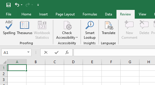
When you need to insert a new column, you must select an existing column and insert the new one below or above it. However, if you have selected a row in your spreadsheet, the insert cell option will be greyed out.
If the insert cell column option is greyed out on Excel, ensure that you have not selected a row in the spreadsheet.
4. Exit Cell Edit Mode.
If you want to insert a new column in Microsoft Excel, your cursor should not be in Cell Edit mode. If you are in cell editing mode, you should exit the mode by pressing the ESC button on your keyboard.
Once done, you’ll notice that the insert cell column option will be available.
5. Check Your Configurations.
The insert column option might not be enabled in your settings, explaining why the feature is greyed out in the toolbar.
Here’s what you need to do:
- First, open Microsoft Excel.
- After that, click on File > Options.
- Go to the Advanced tab afterward and look for the Display Options section.
- Lastly, select All and click OK to save the changes.
Go back to your file and see if the insert cell column option is available.
6. Disable Excel Add-ins.
Microsoft Excel Add-ins are third-party tools that provide extra functionality to your spreadsheet. They can perform various functions, which makes your overall experience better. However, you might be using an add-in that disables the insert cell option.
To rule this out, we suggest disabling any add-in you are using on Excel.
- Launch Microsoft Excel on your computer.
- Next, click on the File tab and choose Options.
- Access the Add–ins tab afterward and disable your add-ins.
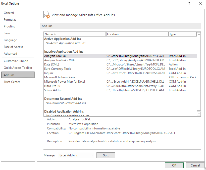
Restart Microsoft Excel and see if the problem is solved.
That ends our guide on what to do if the insert cell column option is greyed out on Microsoft Excel. If you have questions, please drop a comment below, and we’ll do our best to help.
If this guide helped you, please share it. 🙂
Join 50,000+ subscribers
Stay updated on the latest discounts, exclusive promos, and news articles from Saint.
Adding a column in Excel means inserting a new column to the existing dataset. Besides inserting, one may need to delete, hide, unhide, and move rows or columns. Such modifications help in structuring and organizing the dataset. As a result, it is essential to be aware of the techniques related to these alterations.
For example, while preparing a consolidated balance sheet, Mr. X realizes that the data related to the previous year is missing. To include this data, he wants to insert a new column. Here, the method of inserting a column comes into use.
Excel provides different ways of performing actions on a dataset. This article discusses the most appropriate and effective methods of working with data. It covers the following aspects: –
- Insert Excel columns (alternate methods and shortcuts)
- Delete columns and rows
- Hide and unhide rows or columns
- Move rows or columns
Apart from inserting columns in Excel, the remaining topics have been covered in brief.
Table of contents
- How to Add/Insert Columns in Excel?
- Example #1–Add Columns in Excel
- Example #2–Alternate Method to Insert Rows and Columns in Excel
- Example #3–Hide and Unhide Columns & Rows in Excel
- Example #4–Move Rows or Columns in Excel
- Shortcuts to Insert Columns in Excel
- Frequently Asked Questions
- Recommended Articles
How to Add/Insert Columns in Excel?
Below are some examples through which you may learn how to add and insert columns in Excel.
Example #1–Add Columns in Excel
The following table shows the first and the last names in columns A and B, respectively. We want to insert a new column (column B) between these names, which will display the middle name.

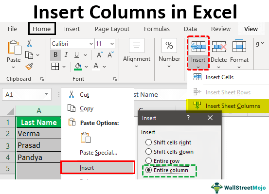
The steps to insert a new column (column B) between two existing columns (columns A and B) are listed as follows:
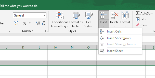
Step 1: Select any cell of column B. Alternatively, one can also select column B, as shown in the following image. Further, click the “Insert” drop-down from the “Home” tab of the Excel ribbonThe ribbon is an element of the UI (User Interface) which is seen as a strip that consists of buttons or tabs; it is available at the top of the excel sheet. This option was first introduced in the Microsoft Excel 2007.read more. Finally, select “Insert Sheet Columns.”
Note: To select a column, click its label or header on top.
Step 2: A new column (column B) is inserted between the columns containing the first and the last names. As a result, the data (last name) of the previous column B (shown in step 1) now shifts to column C.
Note: Excel inserts a column immediately preceding the column of the selected cell. Hence, one must always choose a cell accordingly. If a column is selected, Excel inserts a column preceding it.

Example #2–Alternate Method to Insert Rows and Columns in Excel
Working on the data of example #1, we need to insert a middle name column using the following methods:
a) Select and right-click a cell
b) Select and right-click a column
a) The steps for inserting a column after selecting and right-clicking a cell are listed as follows:
Step 1: Select any cell of column B. This is because a column preceding column B is to be inserted. Right-click the selection and choose “insert,” as shown in the following image.
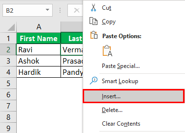
Step 2: The “Insert” dialog box appears. Select “Entire column” to insert a new column.
Note: For inserting a new row, select “Entire row.”
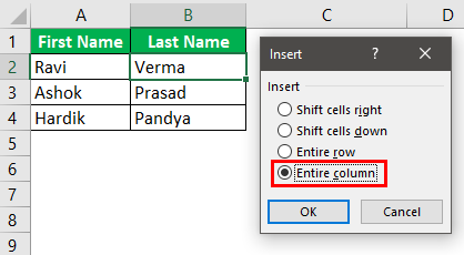
Step 3: A new column (column B) for typing middle names has been inserted.

b) The steps for inserting a column after selecting and right-clicking a column are listed as follows:
Step 1: Select the entire column B. That is because a column preceding column B is to be inserted. Right-click the selection and choose “Insert,” as shown in the following image.
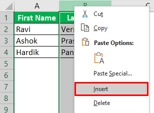
Step 2: A new column B is inserted. The same has been shown under step 3 of method a.
Note: Select the entire row preceding which a new row is inserted for inserting rows. Right-click the selection and choose “Insert.” The same is shown in the following image.

Example #3–Hide and Unhide Columns & Rows in Excel
Working on the data of example #1, we want to perform the following tasks:
a) Hide columns A and B or rows 3 and 4 by right-clicking
b) Hide column A by using the “format” drop-down
c) Unhide columns B and C by right-clicking
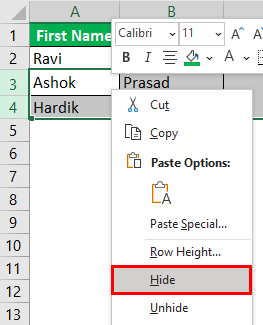
a) The steps to hide the columns A and B or rows 3 and 4 by right-clicking are listed as follows:
Step 1: Select columns A and B. Right-click the selection and choose “hide,” as shown in the next image.
Note 1: To select a row or column, click the row number (to the left) or the column label (on top).
Note 2: Multiple adjacent rows or columns can be selected by dragging across the row and column headings. Alternatively, hold the “Shift” key while selecting the rows or columns.
Note 3: We can select non-adjacent rows or columns by holding the “Ctrl” key while making the selections.
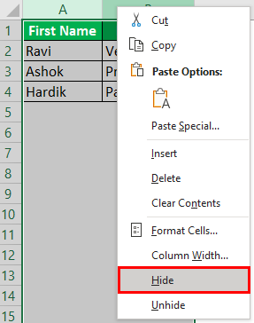
Step 2: Columns A and B will be hidden. Likewise, select rows 3 and 4. Right-click the selection and choose the “Hide” option from the context menu. The same is shown in the following image.
It will hide rows 3 and 4.
b) The steps to hide column A by using the “format” drop-down are listed as follows:
Step 1: Select any cell of column A. Click the “Format” drop-down under the “Home” tab of the Excel ribbon. Next, select “Hide Columns” under the “Hide & Unhide” option.
The same is shown in the following image.
Note: Alternatively, select the relevant column to be hidden. Click “Hide columns” under the “Hide & Unhide” option.
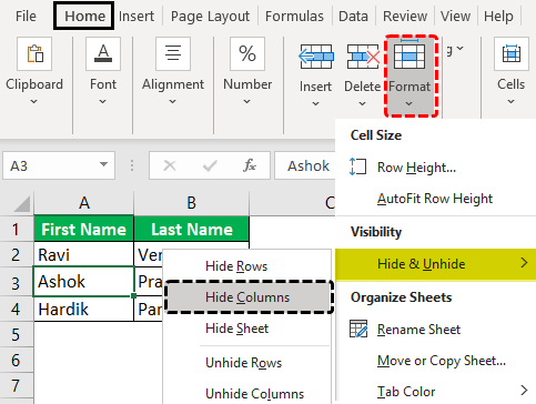
Step 2: We will hide the column of the selected cell, column A. Likewise, to hide rows, select the relevant row. Then, choose “Hide Rows” from the “Hide & Unhide” option of the “Format” drop-down.
c) The steps to unhide columns B and C by right-clicking are listed as follows:
Step 1: Select the unhidden columns (A and D) immediately before and after the hidden columns (B and C). Right-click the selection and choose “Unhide.”
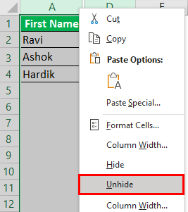
Step 2: The columns B and C will be unhidden. The dataset appears as shown in step 1 of task b.
Likewise, unhide rows by selecting the “Unhide rows” (immediately before and after the hidden rows) and clicking “Unhide” from the context menu.
Example #4–Move Rows or Columns in Excel
Working on the data of example #1, we want to move column B (last name) to precede column A (first name).
The steps to move column B are listed as follows:
Step 1: Select column B, which is to be moved. Cut it in either of the following ways:
- Press “Ctrl+X.”
- Click the scissors icon from the “Clipboard” group of the “Home” tab.
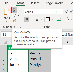
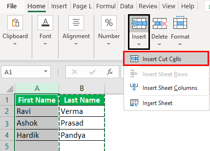
Step 2: Select column A, where the data of column B is to be pasted. Right-click the selection and choose “Insert Cut Cells.”
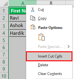
Alternatively, select “Insert Cut Cells” from the “Insert” drop-down of the “Home” tab. The same is shown in the following image.
Note: The “Insert Cut Cells” option will be visible once the selected cells have been cut.
Step 3: The data of column B is pasted into column A. Hence, the first column (column A) now contains the last names. The data of the initial column A (first name) automatically shifts to column B.
The same is shown in the following image.
Note: A row can be selected, cut, and pasted to the desired location. Select the “Insert Cut Cells” option from the “Insert” drop-down of the “Home” tab for pasting.

Shortcuts to Insert Columns in Excel
Let us go through the two shortcuts for inserting columns and rows.
a) Shortcut for inserting with the “Insert” drop-down of the “Home” tab
The excel shortcutAn Excel shortcut is a technique of performing a manual task in a quicker way.read more for inserting a row or column with the “Insert” drop-down works as follows:
- Select a cell preceding which a row or column is inserted.
- Click the “Insert” drop-down from the “Cells” group of the “Home” tab.
- Press “R” to insert a row or “C” to insert a column
A new row or column is inserted depending on the third pointer’s key.
Note: Under the “Insert” drop-down, the “R” of “insert sheet rows” and the “C” of “insert sheet columns” are underlined. Hence, these keys work as shortcuts for inserting rows and columns.
b) Shortcut for inserting with right-click
- The shortcut for inserting a row or column with right-click works as follows:
- Select a cell preceding which a row or column is inserted.
- Right-click the selection and press “I.” The “Insert” dialog box opens.
- Press “R” to insert a row or “C” to insert a column.
- Press the “Enter” key.
A new row or column is inserted depending on the third pointer’s key.
Note: If the “Insert” dialog box does not open in step 2, press the “Enter” key after pressing “I.” It opens the “Insert” dialog box.
Frequently Asked Questions
1. What does it mean to insert a column? How is it done in Excel?
Inserting a column refers to adding a new column to an existing dataset. This new column may contain additional data that can be important for the end-user.
Additionally, there is a possibility that a column has been omitted by mistake. In such cases, inserting a column will be helpful.
The steps to insert a column in Excel are listed as follows:
a. Select the column preceding which a new column is to be inserted.
b. Right-click the selection and choose “Insert” from the context menu.
It will insert the new column immediately before the selected column.
Note: To select a column, click its header (label) on top.
2. How to insert a column in Excel by using a shortcut?
Let us insert a new column E in Excel. The steps to insert a column (column E) by using a shortcut are listed as follows:
a. Select the existing column E.
b. Press the keys “Ctrl+Shift+plus sign(+)” together to insert a column.
It will insert the new column E. The data of the initial column E now shifts to column F.
Note 1: One must select a column carefully. That is because Excel inserts a column preceding the selected column.
Note 2: As an alternative to step a, one can select any cell of column E. After that, press “Ctrl+space” to select the entire column E.
3. How to insert multiple adjacent columns in Excel?
Let us insert columns D, E, and F in Excel. The steps to insert multiple columns (D, E, and F) are listed as follows:
a. Select as many columns in the existing dataset as the number of the new columns to be inserted. So, select the current columns D, E, and F.
b. Press the keys “Ctrl+Shift+plus sign(+)” together.
It will insert the blank columns D, E, and F. The initial columns D, E, and F data shift to columns G, H, and I.
Note 1: Alternative to step a: select adjacent cells of columns D, E, and F. These cells should be in one row. Further, press “Ctrl+space.” As a result, columns D, E, and F will be selected.
Note 2: To select multiple adjacent columns (in step a), drag across the column headings. Alternatively, hold the “Shift” key while selecting the columns.
Note 3: Alternative to step b: right-click the selection and choose “Insert.”
Recommended Articles
This article is a guide to Add Columns in Excel. We also discuss inserting, hiding, and moving rows and columns in Excel and practical examples. You may learn more about Excel from the following articles: –
- Compare Two Columns in Excel for Matches
- 3 Ways to Show Excel Negative Numbers
- Rows vs. Columns
- Move Columns in Excel

Excel Add Column (Table of Contents)
- Add Column in Excel
- How to Add Column in Excel?
- How to Modify a Column Width?
Add Column in Excel
Excel allows a user to add columns, whether left or right, of the column in the worksheet, which is called Add Column in Excel. Of course, there is more than one way to accomplish a task, as in all Microsoft programs. These instructions cover how rows and columns can be added and modified in an Excel worksheet using a keyboard shortcut and using the context menu with the right-click.
How to Add Column in Excel?
Adding a column in Excel is very easy and convenient whenever we want to add data to the table. There are different Methods to Insert or add Column which is as follows:
- Manually we can do this by just right-clicking on the selected column> then click on the insert button.
- Use Shift + Ctrl + + shortcut to add a new column in the Excel.
- Home tab >> click on Insert >> Select Insert Sheet Columns.
- We can add N number of columns in the Excel sheet; a user needs to select that many columns which number of columns he wants to insert.
Let’s understand How to Add Column in Excel with a few examples.
Example #1
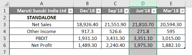
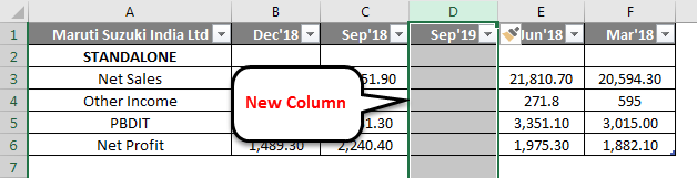
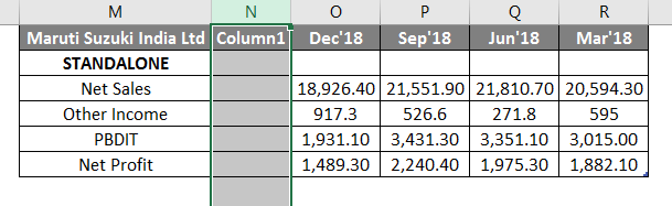
A user has a standalone book data of sales, income, PBDIT, and Profit details of each quarter of Maruti Suzuki India Pvt Ltd in sheet1.
You can download this Add a Column Excel Template here – Add a Column Excel Template
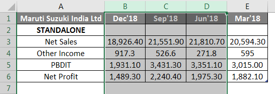
Step 1: Select the column where a user wants to add the column in the excel worksheet (The new column will be inserted to the left of the selected column, so select accordingly)
Step 2: A user has selected the D column where he wants to insert the new column.
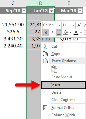
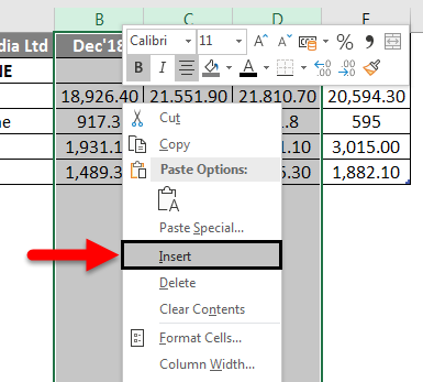
Step 3: Now Right-click and select Insert button or use shortcut Shift + Ctrl + +
Or

As we can see, as it was required to insert a new column between C and D column, in the above example, we have added a new column. So, as a result, it will move the D column data to the next column, which is E, and it will take the place of D.
Example #2
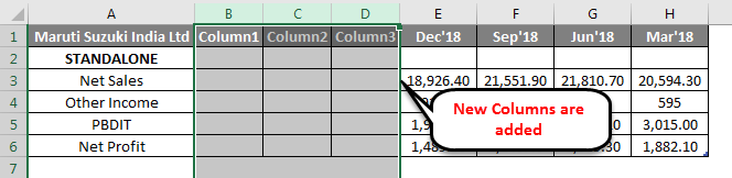
Let’s take the same data to analyze this example. A user wants to insert three columns left of the B column.
Step 1: Select B, C, and D columns where a user wants to insert new 3 columns in the worksheet (The new column is inserted to the left of the selected column, so select accordingly)
Step 2: A user has selected the B, C, and D columns where he wants to insert a new column
Step 3: Now Right-click and select Insert button or use shortcut Shift + Ctrl + +
Or
As we can see, as it was required to insert a new column left of the B, C, and D column, we added a new column in the above example. As a result, it will move B, C, and D column data to the next column, which are E, F, and G; it will take the place of the B, C, and D column.
Example #3
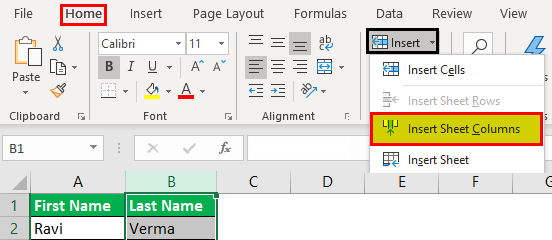
Step 1: Go to Worksheet >> Select the column’s heading where a user wants to insert a new column.
Step 2: Click on the Insert button.
Step 3: One drop-down will be open; click on the Insert Sheet Columns.
As the user wants to use the Insert toolbar to insert a new column, as in the above example, it added.
Example #4
The user can insert a new column in any version of Excel; in the above examples, we can see that we had selected one or more columns in the worksheet then >Right click on the selected column> then clicked on the Insert button.
To add a new column in the excel worksheet.
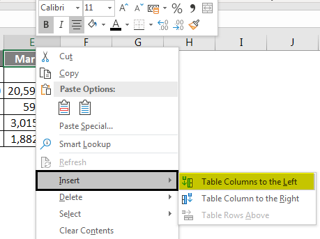
Click in a cell to the left or right of where you want to add a column. If the user wants to add a column to the left of the cell, then follow the below process:
- Click on Table Columns to the Left from the Insert option.
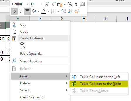
And if a user wants to insert the column to the right of the cell, then follow the below process:
- Click on Table Columns to the Right from the Insert option.
How to Modify a Column Width?
A user can modify the width of any column. Let’s take an example as some of the content in column A cannot be displayed. We can make all this content visible by changing the width of column A.
Step 1: Position the mouse over the column line in the column heading to the Black Cross. (As shown below)
Step 2: Click, hold and drag the mouse to increase or decrease the column width.
Step 3: Release the mouse. The column width will be changed.
A user can auto fit the width of the column. The AutoFit feature will allow you to set a column’s width to fit its content automatically.
Step1: Position the mouse over the column line in the column heading to the Black Cross.
Step2: Double-click the mouse. The column width will be changed automatically to fit the content.
Things to Remember About Add a Column in Excel
- The user needs to select that column where the user wants to insert the new column.
- By default, every row and column have the same height and width, but a user can modify the width of the column and the height of the row.
- The user can insert multiple columns at a time.
- You can also AutoFit the width for several columns at the same time. Simply select the columns you want to AutoFit, and then select the AutoFit Column Width command from the Format drop-down menu on the Home. This method can also be used for row height.
- All the rules will also be applied for rows, as applied to column insertion.
- Excel allows the user to wrap text and merging cells.
- For deleting also, we can go to Home Tab >> Delete >> Delete Sheet Columns; either we can select the column which we want to delete or >> Right Click >> click on Delete.
- After adding the insert column, all the data will be shifted to the right side after that column.
Recommended Articles
This is a guide to add a column in excel. Here we have discussed How to Add a column in excel by using different methods and How to modify a column in Excel along with practical examples and a downloadable excel template. You can also go through our other suggested articles –
- COLUMNS Formula in Excel
- Switching Columns in Excel
- Excel COLUMN to Number
- Freeze Columns in Excel