
Excel for Microsoft 365 Excel for Microsoft 365 for Mac Excel for the web Excel 2021 Excel 2021 for Mac Excel 2019 Excel 2019 for Mac Excel 2016 Excel 2016 for Mac Excel 2013 Excel 2010 Excel 2007 Excel for Mac 2011 Excel Starter 2010 More…Less
This article describes the formula syntax and usage of the COLUMNS
function in Microsoft Excel.
Description
Returns the number of columns in an array or reference.
Syntax
COLUMNS(array)
The COLUMNS function syntax has the following argument:
-
Array Required. An array or array formula, or a reference to a range of cells for which you want the number of columns.
Example
Copy the example data in the following table, and paste it in cell A1 of a new Excel worksheet. For formulas to show results, select them, press F2, and then press Enter. If you need to, you can adjust the column widths to see all the data.
|
Formula |
Description |
Result |
|
=COLUMNS(C1:E4) |
Number of columns in the reference C1:E4. |
3 |
|
=COLUMNS({1,2,3;4,5,6}) |
Number of columns in the array constant {1,2,3;4,5,6}. There are two 3-column rows, containing 1,2, and 3 in the first row and 4,5, and 6 in the second row. |
3 |
Need more help?
Want more options?
Explore subscription benefits, browse training courses, learn how to secure your device, and more.
Communities help you ask and answer questions, give feedback, and hear from experts with rich knowledge.
In Microsoft Excel, a column runs vertically in the grid layout of a worksheet. Vertical columns are numbered with alphabetic values such as A, B, C.Each column in the worksheet has its own column number which is used as part of a cell reference such as A1, A2, or M16.
Contents
- 1 What is column in Excel with example?
- 2 What does column () mean?
- 3 How do you use columns?
- 4 What is difference between column and columns in Excel?
- 5 Where are columns in Excel?
- 6 What is the column number in Excel?
- 7 What does column mean in writing?
- 8 What is column example?
- 9 How do I make columns in Excel?
- 10 What are columns in table?
- 11 What’s column and row?
- 12 How can you tell the difference between rows and Columns?
- 13 Whats a row and column?
- 14 How do you name a column in Excel?
- 15 How do I find a column number?
- 16 What does number of columns mean?
- 17 How do you add columns in sheets?
- 18 What is a column in a data table called?
What is column in Excel with example?
What is the COLUMN Function in Excel? The COLUMN function in Excel is a Lookup/Reference function. This function is useful for looking up and providing the column number of a given cell reference. For example, the formula =COLUMN(A10) returns 1, because column A is the first column.
The Microsoft Excel COLUMN function returns the column number of a cell reference. The COLUMN function is a built-in function in Excel that is categorized as a Lookup/Reference Function.
How do you use columns?
To add columns to a document:
- Select the text you want to format.
- Click the Page Layout tab.
- Click the Columns command. A drop-down menu will appear. Adding columns.
- Select the number of columns you want to insert. The text will then format into columns.
What is difference between column and columns in Excel?
Each row has a unique number that identifies it. A column is a vertical line of cells. Each column has a unique letter that identifies it.
Comparative Table.
| Basis | Excel Rows | Excel Columns |
|---|---|---|
| Range | Rows are ranging from 1 to 1,048,576 | Columns are ranging from A to XFD. |
Where are columns in Excel?
MS Excel is in tabular format consisting of rows and columns. Row runs horizontally while Column runs vertically. Each row is identified by row number, which runs vertically at the left side of the sheet. Each column is identified by column header, which runs horizontally at the top of the sheet.
What is the column number in Excel?
Excel Columns A-Z
| Column Letter | Column Number |
|---|---|
| A | 1 |
| B | 2 |
| C | 3 |
| D | 4 |
What does column mean in writing?
A column is a recurring piece or article in a newspaper, magazine or other publication, where a writer expresses their own opinion in few columns allotted to them by the newspaper organisation.
What is column example?
8. The definition of a column is a vertical arrangement of something, a regular article in a paper, magazine or website, or a structure that holds something up. An example of column is an Excel list of budget items. An example of column is a weekly recipe article.
How do I make columns in Excel?
To insert a single column: Right-click the whole column to the right of where you want to add the new column, and then select Insert Columns. To insert multiple columns: Select the same number of columns to the right of where you want to add new ones. Right-click the selection, and then select Insert Columns.
What are columns in table?
In a relational database, a column is a vertical group of cells within a table.In a table, each column is typically assigned a data type and other constraints which determine the type of value that can be stored in that column. For example, one column might email addresses, another might accept phone numbers.
What’s column and row?
A row is a series of data put out horizontally in a table or spreadsheet while a column is a vertical series of cells in a chart, table, or spreadsheet. Rows go across left to right. On the other hand, Columns are arranged from up to down.
How can you tell the difference between rows and Columns?
The row is an order in which people, objects or figures are placed alongside or in a straight line. A vertical division of facts, figures or any other details based on category, is called column. Rows go across, i.e. from left to right. On the contrary, Columns are arranged from up to down.
Whats a row and column?
Rows are a group of cells arranged horizontally to provide uniformity. Columns are a group of cells aligned vertically, and they run from top to bottom.
How do you name a column in Excel?
Single Sheet
- Click the letter of the column you want to rename to highlight the entire column.
- Click the “Name” box, located to the left of the formula bar, and press “Delete” to remove the current name.
- Enter a new name for the column and press “Enter.”
How do I find a column number?
Show column number
- Click File tab > Options.
- In the Excel Options dialog box, select Formulas and check R1C1 reference style.
- Click OK.
What does number of columns mean?
moreAn arrangement of figures, one above the other. This is a column of numbers: 12.
How do you add columns in sheets?
Step 1: Click anywhere in the column that’s next to where you want your new column. Step 2: Click Insert in the toolbar. Step 2: Select either Column left or Column right. Column left will insert a column to the left of the column you’re currently clicked into.
What is a column in a data table called?
A column can also be called an attribute. Each row would provide a data value for each column and would then be understood as a single structured data value.
The COLUMNS function is a built-in function in Microsoft Excel. It falls under the category of LOOKUP functions in Excel. The COLUMNS function returns the total number of columns in the given array or collection of references. The purpose of the COLUMNS formula in Excel is to know the number of columns in an array of references.
For example, the formula =COLUMNS(A1:E3) will return as 5 since the range A1:E3 has 5 columns, A, B, C, D, and E, respectively.
Table of Contents
- What Is COLUMNS Function In Excel?
- Syntax
- How To Use COLUMNS Formula In Excel?
- Examples
- Important Things To Note
- Frequently Asked Questions
- Columns Function in Excel Video
- Recommended Articles
- The COLUMNS function in excel is used to find the number of columns used in the worksheet.
- The formula of the columns function in excel is =COLUMN(array), where the array is the only mandatory argument.
- The array shows the range of cells for which the number of columns is derived.
- We can choose either a single cell or a range as the value in the array argument.
- It is important to know that the function will return only the number of columns even if the chosen array has multiple rows and columns.
Syntax
- array = This is a required parameter. An array / a formula resulting in an array / a reference to a range of Excel cells for which the number of columns is to be calculated.
The COLUMNS function has only one argument, and it is mandatory.
How To Use COLUMNS Formula In Excel?
You can download this COLUMNS Function Excel Template here – COLUMNS Function Excel Template
The said function is a worksheet (WS) function. As a WS function, columns can be inserted as a part of the formula in a worksheet cell.
Let us look at the examples given below to understand the use of the COLUMNS function in excel.
Examples
Example #1 – Total Columns In A Range
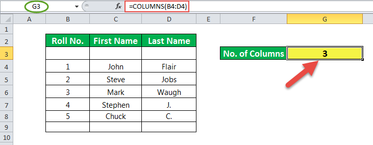
In the example of this column, cell G3 has a formula associated with it. So, G3 is a result cell.
The argument for the COLUMNS function in excel is a cell range, which is B4:D4. Here, B4 is a starting cell, and D4 is the ending cell.
The number of columns between these two cells is 3. So, the result is 3.
Example #2 – Total Cells In A Range

In this example, cell G4 has a formula associated with it. So, G4 is a result cell.
The formula is COLUMNS (B4: E8) * ROWS*B4: E8). Then, multiplication is performed between the total number of columns and a total number of rows for the given range of cells in the sheet.
Here, the total number of columns is four, and the total number of rows is 5. So, the total number of cells is 4*5 = 20.
Example #3 – Get The Address Of The First Cell In A Range

Here, the dataset is named data. Further, this data is used in the formula.
You may refer to the steps given below to name the dataset.
- Step 1: Select the cells.
- Step 2: Right-click and choose Define Name.
- Step 3: Name the dataset as data.

In the example of these columns, cell G6 has a formula associated with it. So, G6 is a result cell. The formula is to calculate the first cell in the dataset represented by the name data. The result is $B$4, i.e., B4, the last cell in the selected dataset.
The formula uses the ADDRESSES function, which has two parameters: row number and column number.
E.g., ADDRESS (8,5) returns $B$4. Here, 4 is the row number, and 2 is the column number. So, the function returns a cell denoted by these row and column numbers.
Here, a row number is calculated by
ROW(data)
And the column number is calculated by
COLUMN(data)
Example 4 – Get The Address Of The Last Cell In A Range

Here, the dataset is named data. Further, this data is used in the column’s formula in Excel. We can refer to the steps given below to name the dataset.
- Step 1: Select the cells.
- Step 2: Right-click and choose Define Name.
- Step 3: Name the dataset as data.

In this COLUMNS example, cell G5 has a formula associated with it. So, G5 is a result cell. The formula is to calculate the last cell in the dataset represented by the name data. The result is $E$8, i.e., E8, the last cell in the selected dataset.
The formula uses the ADDRESSES function, which has two parameters: row number and column number.
E.g., ADDRESS (8,5) returns $E$8. Here, 8 is the row number, and 5 is the column number. So, the function returns a cell denoted by these row and column numbers.
Here, the row number is calculated by
ROW(data)+ROWS(data-1)
And the column number is calculated by
COLUMN(data)+COLUMNS(data-1)
Important Things To Note
- The argument of the COLUMNS function in Excel can be a single cell address or a range of cells.
- The argument of the COLUMNS function cannot point to multiple references or cell addresses.
Frequently Asked Questions
1) What is the columns function in excel?
Columns Function in excel is a built-in excel function used to derive the number of columns used in the worksheet. The syntax of the COLUMNS function in excel is =COLUMNS(array). For example, consider the table with details of 3 employees.
We can calculate the number of columns used in the data using the columns function in excel.
Step 2: Select the range A1:C4 as shown in the below image.
Step 3: Press Enter key
We will get the result as shown in the below image.
2) When can we use the columns function in excel?
Columns Function in excel is used when we have to find the number of columns used in the data. Especially while working with large datasets, this function will be useful.
3) How to insert columns function in excel?
We can insert columns function in excel by selecting Formulas > Lookup & Reference in the Function Library group > COLUMNS function.
Alternatively, we can also type =COLUMNS and choose the cell array.
Columns Function in Excel Video
Recommended Articles
This article is a guide to Columns Function in Excel. We discuss the columns formula in Excel and how to use it, along with examples and downloadable templates. You can also go through our other suggested articles: –
- Excel Column Lock
- Excel Freeze Columns
- Group Column in Excel
- Column in Excel
- Break Links in Excel

Microsoft Excel displays data in tabular format. This means that information is arranged in a table consisting of rows and columns.
Rows and columns are different properties that together make up a table.
These are the two most important features of Excel that allow users to store and manipulate their data.
Below we’ll discuss the definitions of a row and a column, along with the differences between these two features.
Each row is denoted and identified by a unique numeric value that you’ll see on the left hand side.
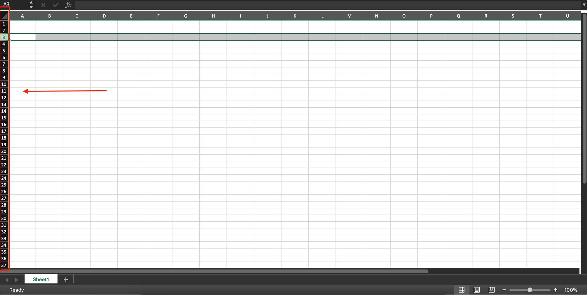
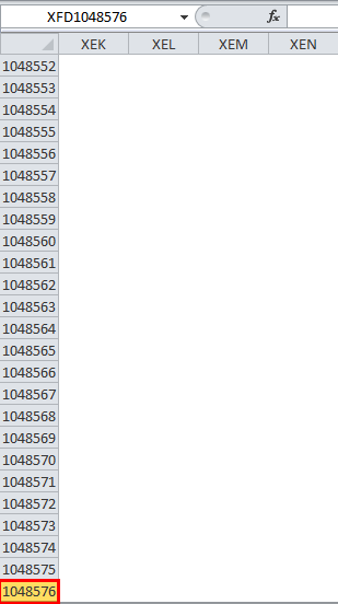
The row numbers are arranged vertically on the worksheet, ranging from 1-1,048,576 (you can have a total of 1,048,576 rows in Excel).
The rows themselves run horizontally on a worksheet.
Data is placed horizontally in the table, and goes across from left to right.
Row 1 is the first row in Excel.
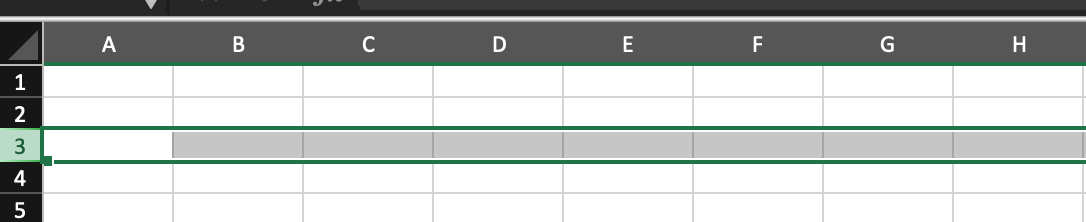
As you can see in the example below, you can select the whole row with the number 3 by clicking on the number itself.
To navigate through the numbers and reach the last row, you can use:
- For Windows Users:
Control down navigation arrow. You first press the Control key and then, while holding it down, press the down navigation arrow. - For Mac Users:
Command down navigation arrow. You first press the Command key and then, while holding it down, press the down navigation arrow.
To get back to the first row (the top) again, press Control up navigation arrow for Windows and Command up navigation arrow for Mac.
What is a column in Excel?
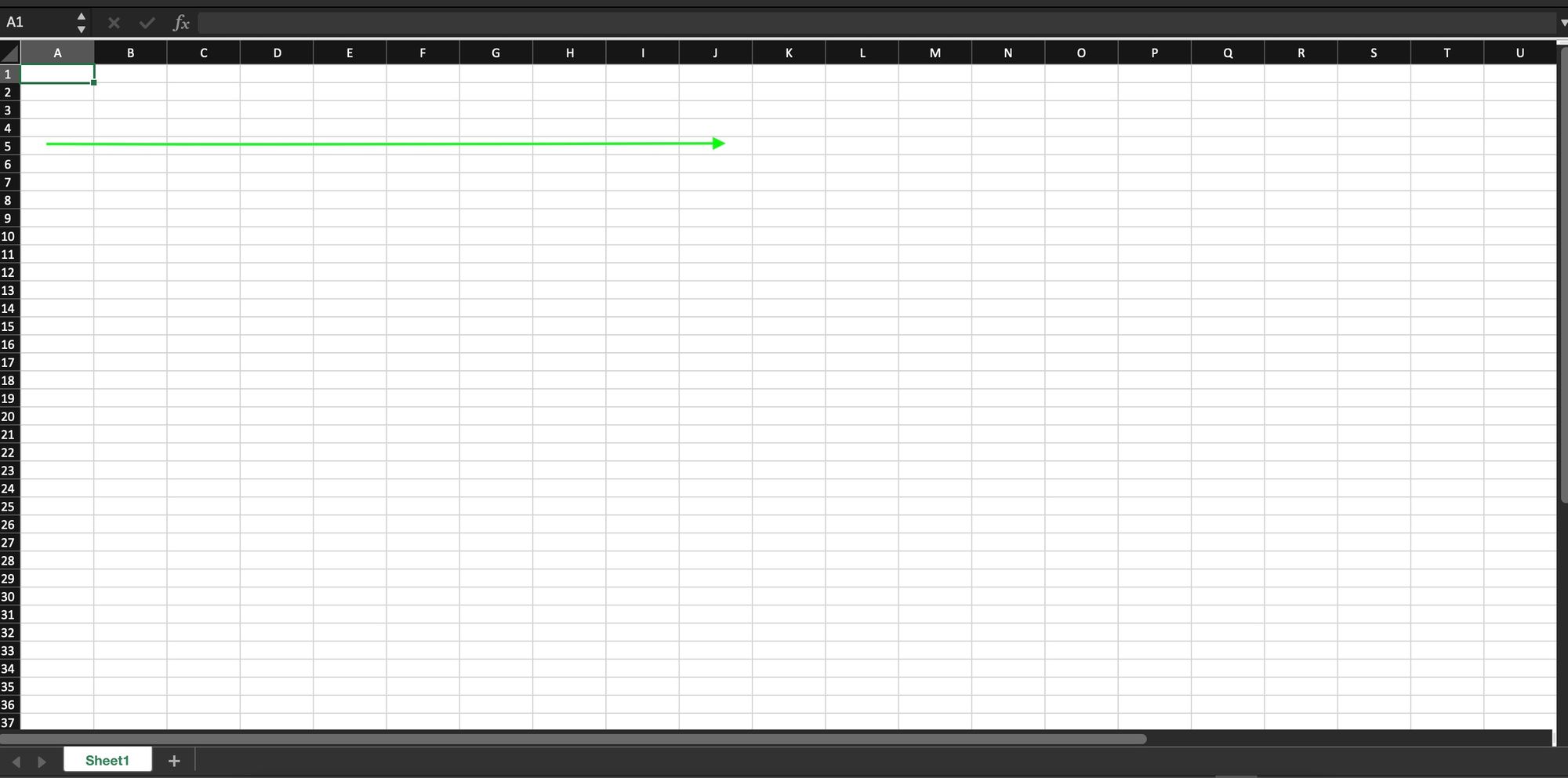
Columns are denoted and identified by a unique alphabetical header letter, which is located at the top of the worksheet.
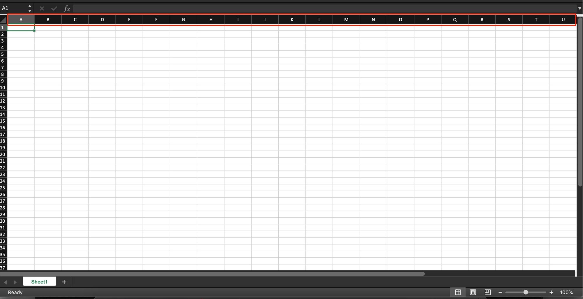
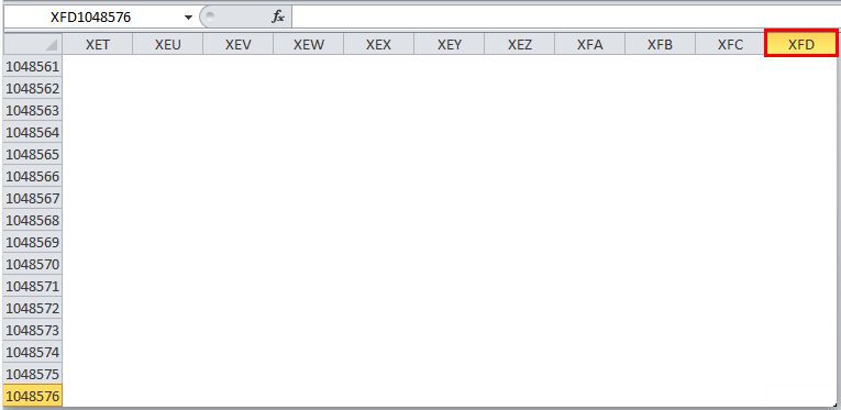
Column headers range from A-XFD, as Excel spreadsheets can have 16,384 columns in total.
Columns run vertically in the worksheet, and the data goes from up to down.
Column A is the first column in Excel.
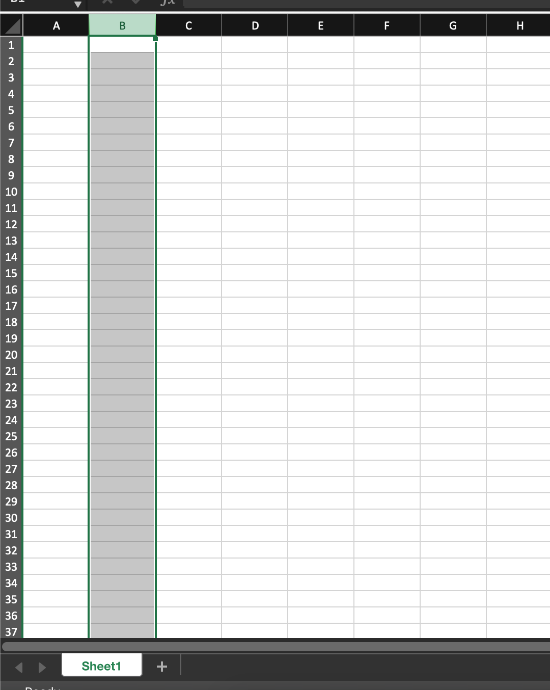
In the example below, you can see that the whole column with header B is selected by pressing/clicking on the letter at the top.
To move to the last column:
- For Windows Users:
Control right navigation arrow. First press the Control key and then, while holding it down, press the right navigation arrow. - For Mac Users:
Command right navigation arrow. First press the Command key and then, while holding it down, press the right navigation arrow.
To get back to the first column again, press Control left navigation arrow for Windows and Command left navigation arrow for Mac.
What is a cell in Excel?
A cell is the intersection of a row and a column. A row and a column adjoined make up a cell.
You can define a cell by the combination of a row number and a column header.
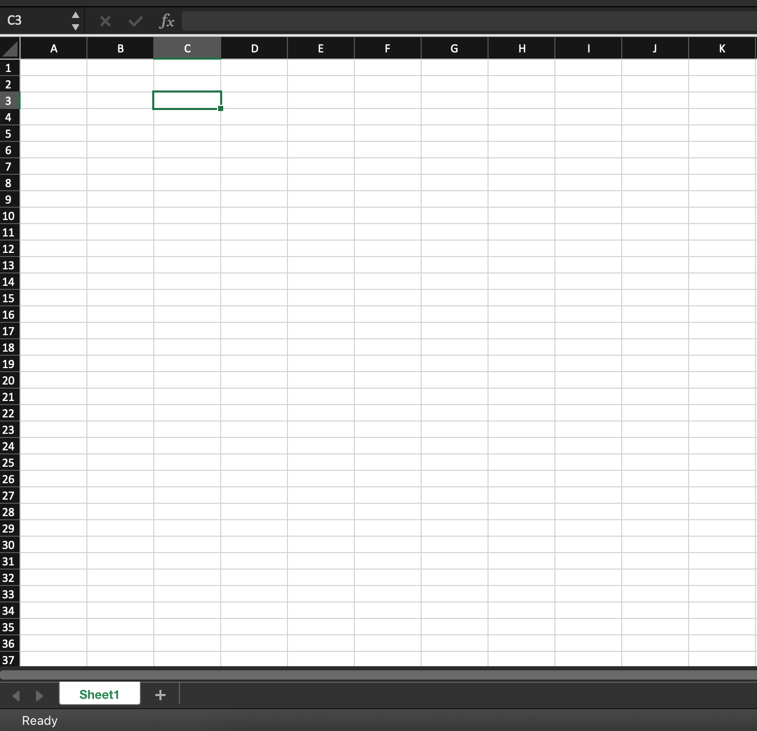
For example, below the selected cell is C3. It has a column header C and a row number 3.
We can also select an entire row or column from a cell.
To select the whole row when in any cell, press Shift Space.
To select the whole column when in any cell, press Ctrl Space.
Conclusion
Now you know the definitions of rows and columns in Excel. You’ve learned their main differences and how they work.
In summary, information in a row is presented horizontally, whereas in a column information is vertical.
Thanks for reading!
Learn to code for free. freeCodeCamp’s open source curriculum has helped more than 40,000 people get jobs as developers. Get started
Rows and Column in Excel (Table of Contents)
- Introduction to Rows and Column in Excel
- Rows and Column Navigation in excel
- How to Select Rows and Column in excel?
- Adjusting Column Width
Introduction to Rows and Column in Excel
In Microsoft excel, if we open a new workbook, we can see that sheet will contain tables with light grey color. Basically excel is a tabular format which contains n number of rows and columns, where rows in excel will be in a horizontal line, and column in excel will be in a vertical line.
- In excel, we can find each row by its row number, which is shown in the below screenshot, which shows vertical numbers on the left side of each sheet.
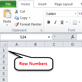
- As we can see in the above screenshot that each row can be identified by their row numbers like 1, 2, 3 etc.
- Whereas we can find the column in excel, which can be identified by the column header like A, B, C. which will be shown normally in all excel sheets, which are shown below.
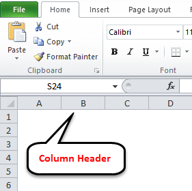
- In Excel, each column is named by its header, which shows the column header horizontally at the top of the excel sheet.
In Microsoft Excel 2010 and the latest version, we have row numbers ranging from 1 to 1048576 in 1048576, whereas the column ranges from A to XFD in a total of 16384 columns which is shown in the below screenshot.
Rows in excel range from 1 to 1048576, which is highlighted in red mark
The column in excel ranges from A to XFD, which is highlighted in red mark.
Rows and Column Navigation in excel
In this example, we will see how to navigate rows and columns with the below examples.
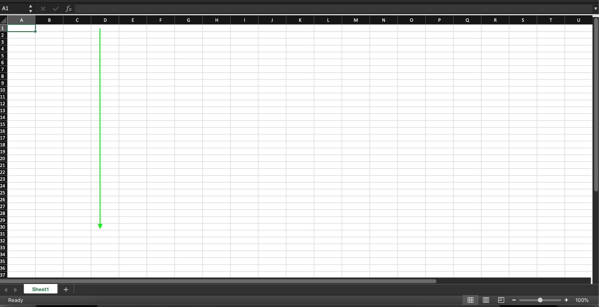
We can find the last row of excel by using the keyboard shortcut key CTRL+DOWN NAVIGATION ARROW KEY, or else we can use the vertical scrollbars to go to the end of the row.
We can find the last column of excel by using the CTRL+RIGHT NAVIGATION ARROW KEY, or else we can use the horizontal scrollbars to go to the end of the column.
How to Select Rows and Column in excel?
In this example, we will learn how to select the rows and columns in excel.
You can download this Rows and Column Excel Template here – Rows and Column Excel Template
Rows and Column in Excel – Example#1
Normally, when we open a workbook, we can see that sheet contains tabular rows and columns where each row is specified by their row number and column specified by their column header.
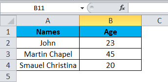
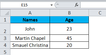
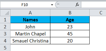
Consider the below example, which has some data in an excel sheet. Here we will see how to select the rows and columns.
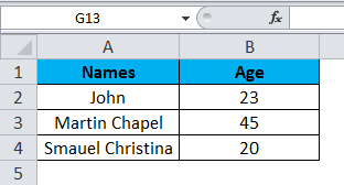
In the above screenshot, we can see that names and age column have their own header name A and B, and each row has its own row number.
In excel, each time when we select a row or column, “Name Box” will display the specific row number and column name, which is shown in the below screenshot.
In this example, we will select the Names and Age, and let’s see how the rows and column header is getting displayed.
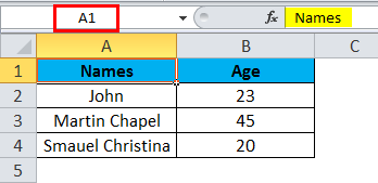
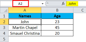
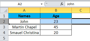
Step 1 – First, select the cell Name John.
Step 2 – Once you select the cell name, John, we will get the row number and column name as A2 in the name box, which means that we have selected A column second row as A2, shown below screenshot with yellow highlighted.
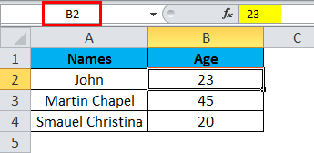
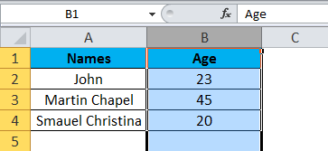
Step 3 – Now select cell 23, where it will show the selected cell is B2 which is shown in the below screenshot with yellow highlighted.
Step 4 – Now select all the names and columns to show that we have 4 rows and 2 columns shown in the below screenshot.
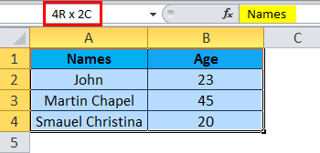
In this way, we can identify the row number and column name by selecting each cell in excel.
Example#2 – Changing Row and Column Size
This example shows how to change the row and column size by using the following examples.
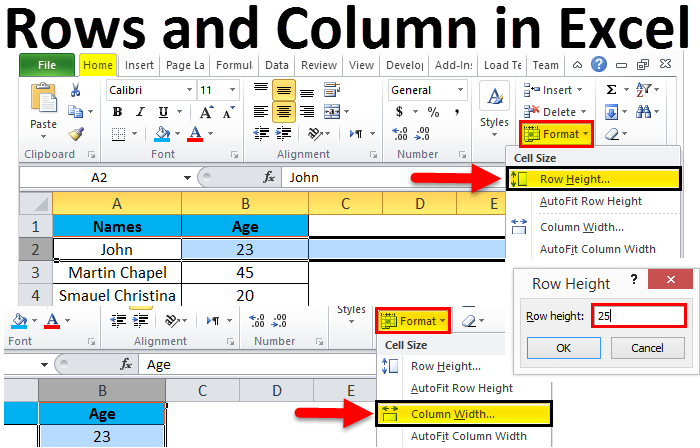
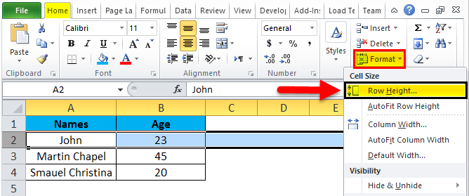
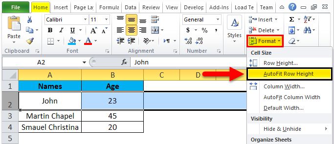
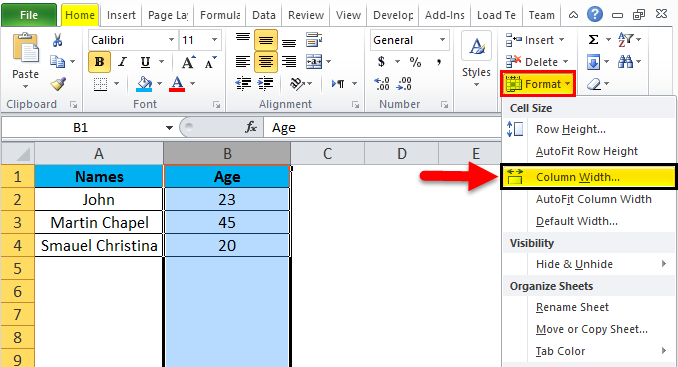
Excel row and column width size can be modified by using the format option in the HOME menu, which is shown below.
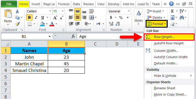
Using the format menu, we can change the row and column width where we have the list option, which are as follows:
- ROW HEIGHT– This is used to adjust the row height.
- AUTOFIT ROW HEIGHT– This will automatically adjust the row height.
- COLUMN WIDTH – This is used to adjust column width.
- AUTOFIT COLUMN WIDTH– This will automatically adjust the column width.
Let’s consider the below example to change the row and column width. Follow the below steps.
Step 1 – First, select the second row as shown in the below screenshot.
Step 2 – Go to the Format menu and click on ROW HEIGHT, as shown below.
Step 3 – Once we select the ROW HEIGHT, we will get the below dialog box to change the height of the row.
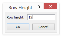
Step 4 – Now increase the row height to 25 so that the selected row height will get increased, as shown in the below screenshot.

We can see that row height has been increased when compared to the previous one; alternatively, we can change the row height by using the mouse.
Step 5 – Now go to the second option in the format list called AUTOFIT ROW HEIGHT, which will automatically reset the row to its original height.
Step 6 – Select the same row and go to the Format menu.
Step 7 – Now select the “AutoFit Row Height” as shown below.
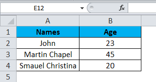
Once we click on the “AutoFit Row Height” option, the row height will reset to the original position, shown below.
Adjusting Column Width
We can adjust the column width in the same way by using the format option.
Step 1 – First, click on the cell B cell as shown below.
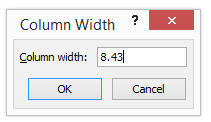
Step 2 – Now go to the Format menu and click on column width as shown in the below screenshot.
Once we click on the Column width, we will get the below dialog box to increase the column width, as shown below.
Step 3 – Now increase the column width by 15 to increase the selected column width.
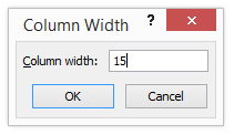
In the above screenshot, we can see that column width has been increased; alternatively, we can adjust the column width by using the mouse where if we place the mouse cursor, we will get the + plus mark sign near to the column.
Step 4 – Now click on the next option called “AutoFit Column width”. So that the selected column will get reset to its original size, which is shown below.
Things to Remember
- In excel, we can delete and insert multiple rows and columns.
- We can hide the specific row and columns using the hide option.
- Row and column cells can be protected by locking the specific cells.
Recommended Articles
This has been a guide to Rows and Columns in Excel. Here we also discuss Rows and Columns in Excel along with practical examples and downloadable excel template. You can also go through our other suggested articles –
- Excel Compare Two Columns
- Unhide Columns in Excel
- Sort Columns in Excel
- Excel Columns to Rows