
Hide or show rows or columns
Hide or unhide columns in your spreadsheet to show just the data that you need to see or print.

Hide columns
-
Select one or more columns, and then press Ctrl to select additional columns that aren’t adjacent.
-
Right-click the selected columns, and then select Hide.
Note: The double line between two columns is an indicator that you’ve hidden a column.
Unhide columns
-
Select the adjacent columns for the hidden columns.
-
Right-click the selected columns, and then select Unhide.
Or double-click the double line between the two columns where hidden columns exist.
Need more help?
You can always ask an expert in the Excel Tech Community or get support in the Answers community.
See Also
Unhide the first column or row in a worksheet
Need more help?
![]()
Download Article
Quickly display one or more hidden columns in your Excel spreadsheet
![]()
Download Article
- Using the Column Drag Tool
- Using Right Click
- Unhiding One Column with the Name Box
- Unhiding All Columns
- Q&A
- Tips
|
|
|
|
|
Are you having trouble viewing certain columns in your Excel workbook? This wikiHow guide shows you how to display a hidden column in Microsoft Excel. You can do this on both the Windows and Mac versions of Excel. There are multiple simple methods to unhide hidden columns. You can drag the columns, use the right-click menu, or format the columns.
Things You Should Know
- Hover your cursor to the right of the hidden columns, then click and drag to the right to unhide them.
- Alternatively, select the columns adjacent to the hidden columns. Then right-click and select Unhide.
- You can also go to Home > Format > Hide & Unhide to show hidden columns.
-

1
Hover your cursor directly to the right of the hidden columns. When your cursor is between the column letters adjacent to the hidden columns, the cursor will change into two parallel lines with two arrows pointing horizontally.
- You can identify hidden columns by looking for two lines between column letters.
- Your cursor needs to be to the right of the two lines for this method. Placing the cursor to the left will increase the column size of the left adjacent column.
-
2
Click and drag to the right. This will unhide the hidden columns between the adjacent columns.
- Alternatively, you can double-click to immediately unhide the hidden column.
Advertisement
-
3


Advertisement
-
1
Select the columns on both sides of the hidden columns. To do this:
- Hold down the ⇧ Shift key while you click both letters above the column
- Click the left column next to the hidden columns.
- Click the right column next to the hidden columns.
- The columns will be highlighted when you successfully select them.
- For example, if column B is hidden, you should click A and then C while holding down ⇧ Shift.
-
2
Right-click either of the selected columns. This will open the right-click pop up menu.
-
3
Select Unhide in the right-click menu. The hidden columns between the two selected columns will be unhidden.
- For more helpful excel tricks, check out our intro guide to Excel.


Advertisement
-
1
Click the Name Box. This is the drop down box to the left of the formula box.[1]
- This method is great for unhiding the first column (A) since there isn’t a column to its left that you can select to access the right-click Unhide menu option.
-
2
Type A1 in the Name Box and press ↵ Enter. Replace A with the letter of the column you want to unhide.
-
3
Click the Home tab. It’s in the upper-left corner of the Excel window.
-
4
Click Find & Select. This is in the «Editing» group in the Home tab. A drop down menu will open.
-
5
Select Go To. This will open the «Go To» window.
-
6
Type A1 in the «Reference» box and click OK.
-
7
Click the Home tab. It’s in the upper-left corner of the Excel window.
-
8
Click Format. This button is in the «Cells» section of the Home tab; you’ll find this section on the right side of the toolbar. A drop down menu will appear.[2]
-
9
Select Hide & Unhide. This option is below the «Visibility» heading in the Format drop down menu. Selecting it will open a pop up menu.
-
10
Click Unhide Columns. It’s near the bottom of the Hide & Unhide menu. Doing so will immediately unhide the column you selected in the Name Box.


Advertisement
-
1
Click the triangle in the top left corner of the spreadsheet. This is next to the row 1 label and column A label. Clicking the triangle will select the entire spreadsheet.
- Hiding columns can be useful for when you have data you don’t need at the moment, but want to keep in the spreadsheet. For example, if you’re tracking your bills in Excel, you might want to hide purchase categories when you’re only working with the sum totals.
-
2
Click the Home tab. It’s in the upper-left corner of the Excel window.
-
3
Click Format. This button is in the «Cells» section of the Home tab; you’ll find this section on the right side of the toolbar. A drop down menu will appear.
-
4
Select Hide & Unhide. This option is below the «Visibility» heading in the Format drop down menu. Selecting it will open a pop up menu.
-
5
Click Unhide Columns. It’s near the bottom of the Hide & Unhide menu. Doing so will immediately unhide every hidden column in the sheet.


Advertisement
Add New Question
-
Question
What do I do if the hidden columns are A and B?

You can select the whole document and do the steps above to retrieve all hidden columns.
-
Question
What do I do if I’ve followed the instructions provided, but I still cannot unhide column A in Excel?
Try unfreezing the column and unhiding, or freezing then unfreezing then unhiding. This process will work.
-
Question
If column A is hidden in excel, how do I find it?
Just use the search bar on top and type there «A1» the hidden column should appear.
See more answers
Ask a Question
200 characters left
Include your email address to get a message when this question is answered.
Submit
Advertisement
-
If some columns are still not visible after you’ve attempted to unhide the columns, the width of the columns may be set to «0» or another small value. To widen the column, position your cursor on the right border of the column, and drag the column to increase its width.
-
If you want to unhide all hidden columns on an Excel spreadsheet, click on the «Select All» button, which is the blank rectangle to the left of column «A» and above row «1.» You can then proceed with the remaining steps in this article to unhide those columns.
Thanks for submitting a tip for review!
Advertisement
About This Article
Article SummaryX
1. Open your Excel document.
2. Select the columns on both sides of the hidden column.
3. Click Home
4. Click Format
5. Select Hide & Unhide
6. Click Unhide Columns
Did this summary help you?
Thanks to all authors for creating a page that has been read 666,342 times.
Is this article up to date?
Watch Video – How to Unhide Columns in Excel
If you prefer written instruction instead, below is the tutorial.
Hidden rows and columns can be quite irritating at times.
Especially if someone else has hidden these and you forget to unhide it (or even worse, you don’t know how to unhide these).
While I can’t do anything about the first issue, I can show you how to unhide columns in Excel (the same techniques can also be used to unhide rows).
It may happen that one of the methods of unhiding columns/rows may not work for you. In that case, it is good to know the alternatives that can work.
There are many different situations where you may need to unhide the columns:
- Multiple columns are hidden and you want to unhide all columns at once
- You want to unhide a specific column (in between two columns)
- You want to unhide the first column
Let’s go through each for these scenarios and see how to unhide the columns.
Unhide All Columns At One Go
If you have a worksheet that has multiple hidden columns, you don’t need to go hunt each one and bring it to light.
You can do that all in one go.
And there are multiple ways to do this.
Using the Format Option
Here are the steps to unhide all columns at one go:
- Click on the small triangle at the top left of the worksheet area. This will select all the cells in the worksheet.
- Right-click anywhere in the worksheet area.
- Click on Unhide.
No matter where that pesky column is hidden, this will unhide it.
Note: You can also use the keyboard shortcut Control A A (hold the control key and hit the A key twice) to select all the cells in the worksheet.
Using VBA
If you need to do this often, you can also use VBA to get this done.
The below code will unhide column in the worksheet.
Sub UnhideColumns ()
Cells.EntireColumn.Hidden = False
EndSub
You need to place this code in the VB Editor (in a module).
If you want to learn how to do this with VBA, read a detailed guide on how to run a macro in Excel.
Note: To save time, you can save this macro in the Personal Macro Workbook and add it to the quick access toolbar. This will allow you to unhide all columns with a single click.
Using a Keyboard Shortcut
If you’re more comfortable using keyboard shortcuts, there is a way to unhide all columns with a few keystrokes.
Here are the steps:
- Select any cell in the worksheet.
- Press Control-A-A (hold the control key and press A twice). This will select all the cells in the worksheet
- Use the following shortcut – ALT H O U L (one key at a time)
If you can get hang of this keyboard shortcut, it could be a lot faster to unhide columns.
Note: The reason you need to press A twice when holding the control key is that sometimes when you press Control A, it only selects the used range in Excel (or the area that has the data) and you need to press the A again to select the entire worksheet.
Another keyword shortcut that works for some and not for others is Control 0 (from a numeric keypad) or Control Shift 0 from a non-numeric keypad. It used to work for me earlier but doesn’t work anymore. Here is some discussion on why it may happen. I suggest you use the longer (ALT HOUL) shortcut that works every time.
Unhide Columns in Between Selected Columns
There are multiple ways you can quickly unhide columns in between selected columns. The methods shown here are useful when you want to unhide a specific column(s).
Let’s go through these one-by-one (and you can choose to use that you find the best).
Using a Keyboard Shortcut
Below are the steps:
- Select the columns that contain the hidden columns in between. For example, if you are trying to unhide column C, then select column B and D.

- Use the following shortcut – ALT H O U L (one key at a time)

This will instantly unhide the columns.
Using the Mouse
One quick and easy way to unhide a column is to use the mouse.
Below are the steps:
Using the Format Option in the Ribbon
Under the home tab in the ribbon, there are options to hide and unhide columns in Excel.
Here is how to use it:
Another way of accessing this option is by selecting the columns and right clicking using the mouse. In the menu that appears, select the unhide option.

Using VBA
Below is the code that you can use to unhide columns in between the selected columns.
Sub UnhideAllColumns()
Selection.EntireColumn.Hidden = False
End Sub
You need to place this code in the VB Editor (in a module).
If you want to learn how to do this with VBA, read a detailed guide on how to run a macro in Excel.
Note: To save time, you can save this macro in the Personal Macro Workbook and add it to the quick access toolbar. This will allow you to unhide all columns with a single click.
By Changing the Column Width
There is a possibility that none of these methods work when you try to unhide column in Excel. It happens when you change the Column Width to 0. In that case, even if you unhide the column, it’s width still remains 0, and hence you can’t see it or select it.
Below are the steps to change the column width:
This is by far the most reliable way to unhide columns in Excel. If everything fails, just change the column width.
Unhide the First Column
Unhiding the first column can be a little bit tricky.
You can use many of the methods covered above, with a little bit of extra work.
Let me show you a few ways.
Use the Mouse to Drag the First Column
Even when the first column is hidden, Excel allows you to select it and drag it to make it visible.
To do this, hover the cursor on the left edge of column B (or whatever is the leftmost visible column).
The cursor would change into a double arrow pointer as shown below.

Hold the left mouse button and drag the cursor to the right. You will see that it unhides the hidden column.

Go to a Cell in the First Column and Unhide it
But how do you go to any cell in the column that’s hidden?
Good question!
You use the Name Box (it’s left to the formula bar).

Enter A1 in the Name Box. It will instantly take you to the A1 cell. Since the first column is hidden, you won’t be able to see it, but be assured that it’s selected (you’ll still see a thin line just left of B1).
Once the hidden column cell is selected, follow the below steps:
- Click the Home tab.
- In the Cells group, click on Format.
- Hover the cursor on the ‘Hide & Unhide’ option.
- Click on ‘Unhide Columns’
Select the First Column and Unhide it
Again! How do you select it when it’s hidden?
Well, there are many different ways to skin the cat.
And this is just another method in my kitty (this is the last cat sounding reference I promise).
When you select the leftmost visible cell and drag the cursor to the left (where there are row numbers), you end up selecting all the hidden columns (even when you don’t see it).

Once you have select all the hidden columns, follow the below steps:
- Click the Home tab.
- In the Cells group, click on Format.
- Hover the cursor on the ‘Hide & Unhide’ option.
- Click on ‘Unhide Columns’
Check The Number of Hidden Columns
Excel has an ‘Inspect Document’ feature that is meant to quickly scan the workbook and give you some details about it.
And one of the things that you can do that ‘Inspect Document’ is to quickly check how many hidden columns or hidden rows are there in the workbook.
This might be useful when you get the workbook from someone and want to quickly inspect it.
Below are the steps on how to check the total number of hidden columns or hidden rows:
- Open the workbook
- Click on the File tab
- In the Info options, click on the ‘Check for Issues’ button (it’s next to the Inspect Workbook text).

- Click on Inspect Document.

- In the Document Inspector, make sure Hidden Rows and Columns option is checked.

- Click the Inspect button.
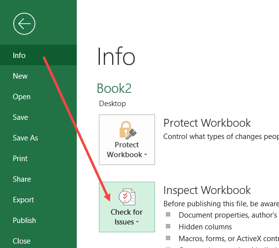


This will show you the total number of hidden rows and columns.

It also gives you the option to delete all these hidden rows/columns. This can be the case if there is extra data that has been hidden and is not needed. Instead of finding hidden rows and columns, you can quickly delete these from this option.
You May Also Like the following Excel Tips/Tutorials:
- How to Insert Multiple Rows in Excel – 4 Methods.
- How to Quickly Insert New Cells in Excel.
- Keyboard & Mouse Tricks that will Reinvent the Way You Excel.
- How to Hide a Worksheet in Excel.
- How to Unhide Sheets in Excel (All In One Go)
- Excel Text to Columns (7 Amazing things you can do with it)
- How to Lock Cells in Excel
- How to Lock Formulas in Excel
Hiding Excel Column(s)
Hiding a column in excel implies making it invisible so that it is removed from display. A hidden column is not deleted from the worksheet. This means that it does exist and has been only temporarily held from view. In Excel, one can hide both contiguous and non-contiguous columns. However, to use a hidden column again, it needs to be unhidden at first.
For example, a column containing calculations may be hidden. This helps avoid confusion amongst users of a shared worksheet.
A column is hidden when its data needs to be concealed from other Excel users, it is unused and not required for a while, its presence is making comparisons between the remaining columns difficult, and so on. The purpose of hiding an excel column is to allow viewing the relevant areas of a worksheet at a given time.
Table of contents
- Hiding Excel Column(s)
- How to Hide Columns in Excel? (Top 4 Methods)
- Example #1–Hide Columns Using the “Hide” Option of the Context Menu
- Example #2–Hide Excel Columns Using the “Ctrl+Zero (0)” Shortcut
- Example #3–Hide Excel Columns by Setting the Column Width as Zero
- Example #4–Hide Columns Using VBA Code
- Frequently Asked Questions
- Recommended Articles
- How to Hide Columns in Excel? (Top 4 Methods)
How to Hide Columns in Excel? (Top 4 Methods)
The techniques of hiding columns in Excel are listed as follows:
- “Hide” option of the context menu
- “Ctrl+zero (0)” shortcut
- Column width as zero
- VBA code
Let us discuss these methods one by one with the help of examples.
Note: All the following examples demonstrate the process of hiding adjacent (contiguous) columns. For hiding multiple non-adjacent columns, refer to the second question under the heading “frequently asked questions.” This is given at the end of this article.
Example #1–Hide Columns Using the “Hide” Option of the Context Menu
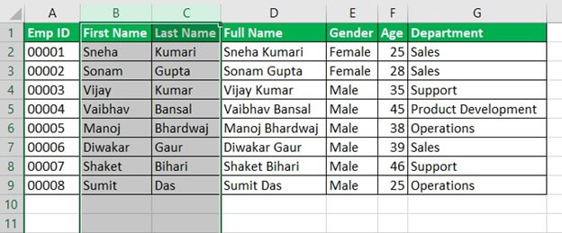
The following table displays the IDs, names, gender, age, and department of some employees of an organization. Consider one column of the table as one column of an Excel worksheet. So, the dataset begins from column A (emp ID) and ends with column G (department).
The first name (column B) and last name (column C) have been concatenated (joined) to form the full name (column D). Since columns B and C are not required (for some time), we want to hide them using the “hide” option of the context menu.
| Emp ID | First Name | Last Name | Full Name | Gender | Age | Department |
|---|---|---|---|---|---|---|
| 00001 | Sneha | Kumari | Sneha Kumari | Female | 25 | Sales |
| 00002 | Sonam | Gupta | Sonam Gupta | Female | 28 | Sales |
| 00003 | Vijay | Kumar | Vijay Kumar | Male | 35 | Support |
| 00004 | Vaibhav | Bansal | Vaibhav Bansal | Male | 45 | Product Development |
| 00005 | Manoj | Bhardwaj | Manoj Bhardwaj | Male | 38 | Operations |
| 00006 | Diwakar | Gaur | Diwakar Gaur | Male | 39 | Sales |
| 00007 | Shaket | Bihari | Shaket Bihari | Male | 46 | Support |
| 00008 | Sumit | Das | Sumit Das | Male | 25 | Operations |
The steps to hide excel columns is listed as follows:
- With the help of the mouse, click the label of column B appearing on top. This selects column B entirely. Next, press the keys “Shift+right arrow” to select the entire column C.
The selection is shown in the succeeding image. Notice that in column A, the numbers have been formatted as text. This has been done to place zeros before each number in cells A2 to A9.
Note 1: For “Shift+right arrow” to work, hold the “Shift” key, and at the same time, press the right arrow. When the shortcut “Shift+right arrow” is pressed after selecting a column, the selection is extended to an adjacent column on the right.
When the shortcut “Shift+right arrow” is pressed after selecting a cell, the selection is extended to an adjacent cell on the right.
Note 2: When the numbers of column A were formatted as text, green triangles (shown in the first image of example #2) had appeared on the upper-left corner of each cell. From the “trace error” button, we clicked “ignore error” (for each cell) to remove such green triangles.

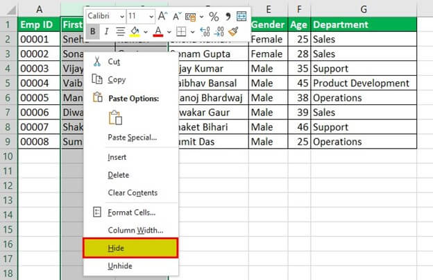
- Right-click the selection and choose “hide” from the context menu. The same is shown in the following image.

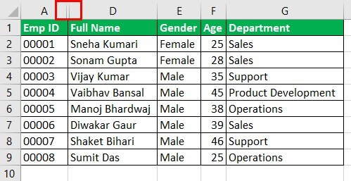
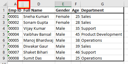
- The final dataset, with columns B and C hidden, is shown in the following image. Notice that there are double vertical lines (shown in a red box) between the column labels A and D. These lines indicate that columns B and C have been hidden.
Another indication of hidden excel columns is the change in the sequence of the column labels. After label A, labels B and C are skipped, and straightaway label D is displayed.

Example #2–Hide Excel Columns Using the “Ctrl+Zero (0)” Shortcut
The following image shows a dataset similar to that of example #1. Notice that the number of columns has been reduced this time. Columns A to D are displayed, which consist of the employee ID, first name, last name, and full name respectively.
Ignore the green triangles in column A of the subsequent images. These are displayed because the “ignore error” option from the “trace error” button has not been clicked, unlike in step 1 of the preceding example (example #1).
We want to hide columns B and C by using the shortcut “Ctrl+zero (0)” in Excel.

The steps to hide the stated columns using the given technique are listed as follows:
Step 1: Select columns B and C, which need to be hidden. For this, click the label of column B with the mouse and drag it across to column C. When the mouse pointer is placed on the label of column B, it changes to an arrow pointing downwards.
Note: Alternatively, select any cell of column B and press the keys “Ctrl+space” together. Column B is selected entirely. Next, press the keys “Shift+right arrow” to select column C.
Step 2: Once the columns to be hidden (columns B and C) are selected, press the keys “Ctrl+zero (0)” together.
The steps 1 and 2 are shown in the following image. Hence, columns B and C (selected in step 1) are hidden. Notice that, in the final output, the double vertical lines separate the labels of columns A and D.
Example #3–Hide Excel Columns by Setting the Column Width as Zero
Working on the dataset of example #2, we want to hide columns B and C by setting the column widthA user can set the width of a column in an excel worksheet between 0 and 255, where one character width equals one unit. The column width for a new excel sheet is 8.43 characters, which is equal to 64 pixels.read more as zero.
The steps to hide the mentioned columns using the given technique are listed as follows:
Step 1: Select the columns to be hidden. So, select columns B and C entirely.
Step 2: Right-click the selection and choose “column width” from the context menu. Set column width as zero and click “Ok.”
Both steps 1 and 2 are shown in the following image. The final dataset, with columns B and C hidden, is also displayed in this image. Double vertical lines appear between the labels of columns A and D.
Note: When a column’s width is entered as zero, the column is hidden from the worksheet.
Example #4–Hide Columns Using VBA Code
Working on the dataset of example #1, we want to hide columns B and C with the help of a VBA codeVBA code refers to a set of instructions written by the user in the Visual Basic Applications programming language on a Visual Basic Editor (VBE) to perform a specific task.read more. Consider the dataset to be in “sheet1” of Excel.
The steps to hide columns using a VBA code are listed as follows:
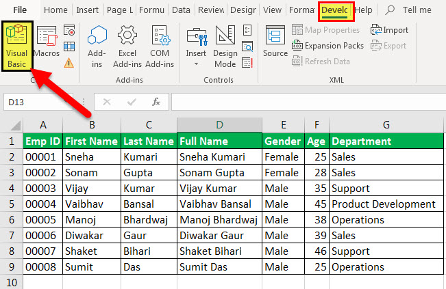
Step 1: From the Developer tab, click “visual basic.” This is shown in the following image.
Note: If the Developer tabEnabling the developer tab in excel can help the user perform various functions for VBA, Macros and Add-ins like importing and exporting XML, designing forms, etc. This tab is disabled by default on excel; thus, the user needs to enable it first from the options menu.read more is not displayed on the ribbon, it must be enabled from the File tab. For the detailed steps, click the given hyperlink.
Step 2: A new window titled “Microsoft visual basic for applications” opens. Double-click “sheet1.” Next, from the Insert tab, click “procedure.” Specify the name of the procedure and paste the following code:
Worksheets(“Sheet1”).Columns(“B:C”).Hidden = True
This is shown in the following image.

Step 3: Save the file with the .xlsm extension as it supports macros. This extension is used for a macro-enabled workbook, which has been created in Excel 2007 or the newer Excel versions.
Step 4: From the Run tab, click “run sub/user form.” The output is shown in the following image. Notice the double line (shown in a red box) between the column labels A and D. This indicates that the columns in between (i.e., columns B and C) are hidden.
Frequently Asked Questions
1. What does it mean to hide columns and how is it done in Excel?
To hide a column means removing one or more excel columns from the display. Such hidden columns do exist in the worksheet even though they become invisible. Columns are usually hidden when they are neither being used nor meant to be deleted.
The steps to hide a column in Excel are listed as follows:
a. Select the column to be hidden.
b. Right-click the selection and choose “hide” from the context menu.
The column selected in step “a” is hidden.
Note: For more techniques of hiding a column, refer to the examples of this article.
2. How to hide multiple columns in Excel?
The steps to hide multiple columns in Excel are listed as follows:
a. Select all the columns that need to be hidden.
• For selecting multiple contiguous columns, drag across the column labels with the mouse. Alternatively, select the first column and press the keys “Shift+right arrow” to select columns on the right.
• For selecting multiple non-contiguous columns, click the first column label. Thereafter, hold the “Ctrl” key and click the other column labels.
b. From the Home tab, click the “format” drop-down in the “cells” group.
c. Under “visibility,” select “hide & unhide.” Next, choose “hide columns.”
The columns selected in step “a” are hidden.
3. How to hide and lock columns in Excel?
The steps to hide and lock columns in Excel are listed as follows:
a. Select the entire worksheet by pressing either the keys “Ctrl+A” or the “select all” button. The “select all” button is located at the top-left corner of the Excel worksheet.
b. Right-click the selection and choose “format cells” from the context menu. The “format cells” dialog box opens. Uncheck the “locked” option in the “protection” tab. Click “Ok.”
c. Select the columns to be hidden and locked. Open the “format cells” dialog box again and click the “protection” tab. Check the “locked” option and click “Ok.”
d. Hide the columns selected in the preceding step (step c). For this, keep the columns to be hidden selected and click the “format” drop-down from the Home tab. Next, click “hide columns” from the “hide & unhide” option.
e. From the Review tab, click “protect sheet.” The “protect sheet” dialog box opens. Keep the following checkboxes selected:
• “Protect worksheet and contents of locked cell”
• “Select locked cells”
• “Select unlocked cells”
f. Enter a password and confirm it. Click “Ok” to proceed. The “protect sheet” dialog box closes.
The columns selected in step “c” are hidden. Since the worksheet is protected, these hidden columns cannot be unhidden by the usual ways to unhide a column. The advantage of locking hidden columns is that their content is concealed from the other users of the worksheet.
Note: To unhide the hidden columns, unprotect the sheet in the first place. To unprotect the sheet, click “unprotect sheet” from the Review tab. Next, enter the password and click “Ok.”
Thereafter, unhide the columns by selecting, right-clicking, and choosing “unhide” from the context menu. Alternatively, select the columns and choose “unhide columns” from the “hide & unhide” option of the “format” drop-down (in the Home tab).
Recommended Articles
This has been a guide to hiding columns in excel. Here we discuss the top 4 methods to hide columns in Excel, including the “hide” option of the context menu, shortcut (Ctrl+0), column width (as zero), and VBA code. You can learn more about Excel from the following articles –
- VBA Hide Columns
- Excel Hide Shortcut
- How to Unhide Columns in Excel?
- How to Freeze or Lock Multiple Columns in Excel?
- FLOOR Function in Excel
Содержание
- Показ скрытых столбцов
- Способ 1: ручное перемещение границ
- Способ 2: контекстное меню
- Способ 3: кнопка на ленте
- Вопросы и ответы

При работе в Excel иногда требуется скрыть столбцы. После этого, указанные элементы перестают отображаться на листе. Но, что делать, когда снова нужно включить их показ? Давайте разберемся в этом вопросе.
Показ скрытых столбцов
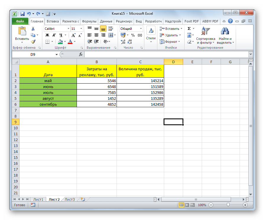
Прежде, чем включить отображение скрытых столбов, нужно разобраться, где они располагаются. Сделать это довольно просто. Все столбцы в Экселе помечены буквами латинского алфавита, расположенными по порядку. В том месте, где этот порядок нарушен, что выражается в отсутствии буквы, и располагается скрытый элемент.
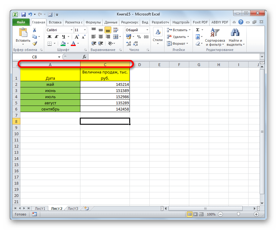
Конкретные способы возобновления отображения скрытых ячеек зависят от того, какой именно вариант применялся для того, чтобы их спрятать.
Способ 1: ручное перемещение границ
Если вы скрыли ячейки путем перемещения границ, то можно попытаться показать строку, переместив их на прежнее место. Для этого нужно стать на границу и дождаться появления характерной двусторонней стрелки. Затем нажать левую кнопку мыши и потянуть стрелку в сторону.
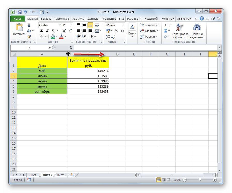
После выполнения данной процедуры ячейки будут отображаться в развернутом виде, как это было прежде.
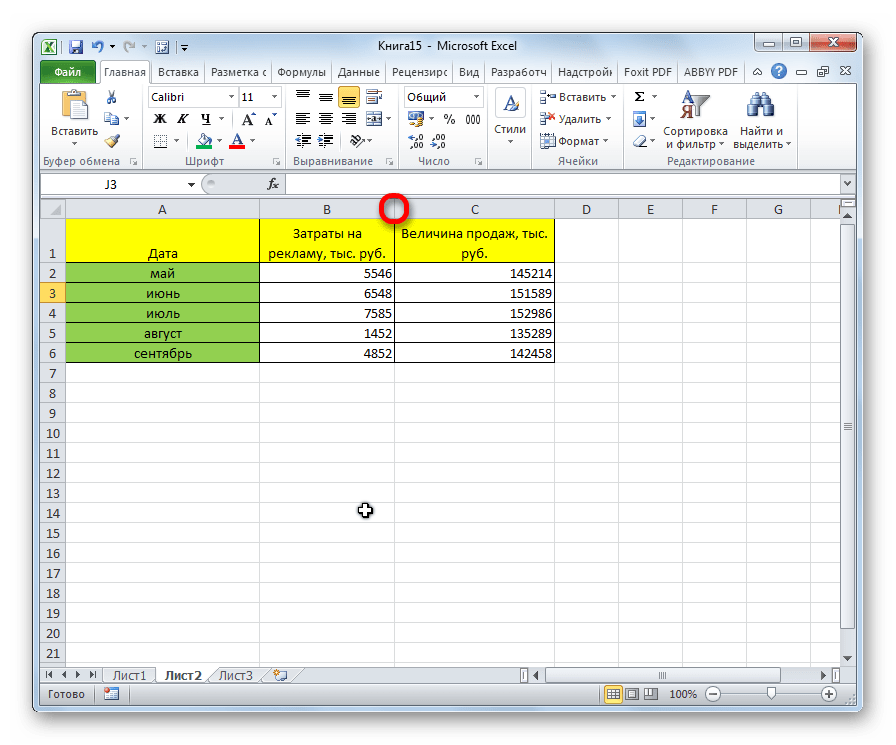
Правда, нужно учесть, что если при скрытии границы были подвинуты очень плотно, то «зацепиться» за них таким способом будет довольно трудно, а то и невозможно. Поэтому, многие пользователи предпочитают решить этот вопрос, применяя другие варианты действий.
Способ 2: контекстное меню
Способ включения отображения скрытых элементов через контекстное меню является универсальным и подойдет во всех случаях, без разницы с помощью какого варианта они были спрятаны.
- Выделяем на горизонтальной панели координат соседние секторы с буквами, между которыми располагается скрытый столбец.
- Кликаем правой кнопкой мыши по выделенным элементам. В контекстном меню выбираем пункт «Показать».
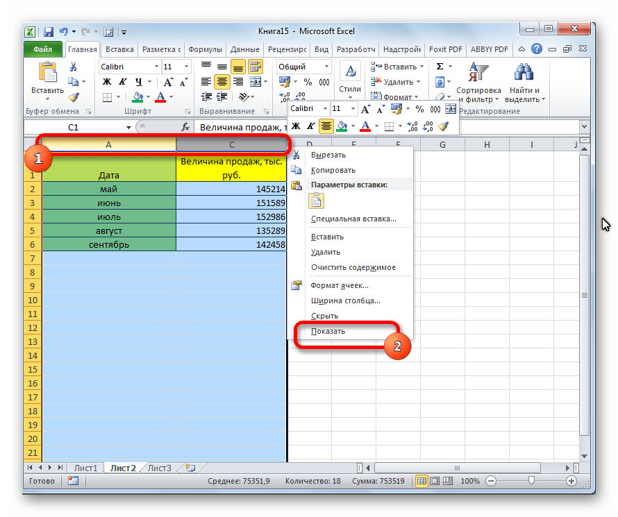
Теперь спрятанные столбцы начнут отображаться снова.
Способ 3: кнопка на ленте
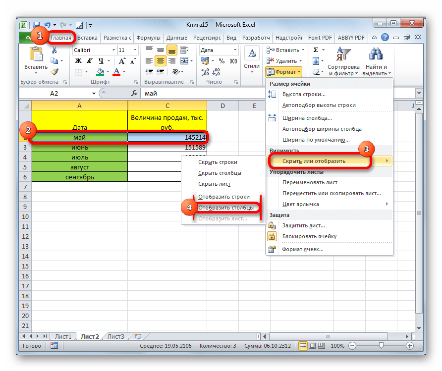
Использование кнопки «Формат» на ленте, как и предыдущий вариант, подойдет для всех случаев решения поставленной задачи.

- Перемещаемся во вкладку «Главная», если находимся в другой вкладке. Выделяем любые соседние ячейки, между которыми находится скрытый элемент. На ленте в блоке инструментов «Ячейки» кликаем по кнопке «Формат». Открывается меню. В блоке инструментов «Видимость» перемещаемся в пункт «Скрыть или отобразить». В появившемся списке выбираем запись «Отобразить столбцы».
- После этих действий соответствующие элементы опять станут видимыми.
Урок: Как скрыть столбцы в Excel
Как видим, существует сразу несколько способов включить отображение скрытых столбцов. При этом, нужно заметить, что первый вариант с ручным перемещением границ подойдет только в том случае, если ячейки были спрятаны таким же образом, к тому же их границы не были сдвинуты слишком плотно. Хотя, именно этот способ и является наиболее очевидным для неподготовленного пользователя. А вот два остальных варианта с использованием контекстного меню и кнопки на ленте подойдут для решения данной задачи в практически любой ситуации, то есть, они являются универсальными.
Еще статьи по данной теме:
Помогла ли Вам статья?

You can hide rows and columns in Excel, and it’s usually easy to unhide those rows or columns later. But, if you run into problems, these quick tips might help you show those rows and columns again.
Unhiding Rows and Columns
If you notice that rows are hidden in an Excel workbook, you can usually unhide them by following these steps:
- Select the rows on either side of the hidden ones
- Next, right-click on one of the selected rows
- In the pop-up menu, click the Unhide command

Trouble Unhiding Top Rows
Occasionally, you can run into problems when you need to unhide rows or column on an Excel worksheet.
For example, if Row 1 is hidden, or the top few rows are hidden, how can you unhide them?
Here are the steps to show the hidden top rows on a worksheet:
- At the left side of the Excel sheet, press on the first visible row button
- In the animated screen shot below, Row 6 is the first visible row
- Next, drag up, onto the Select All button.
- Tips: As you drag up, a small popup appears, to show the number of rows you’ve selected.
- Then, right-click the first visible row button
- In the pop-up menu, click Unhide
This animated gif shows the steps for selecting the hidden rows at the top of a worksheet, and unhiding them

Another Hidden Top Rows Fix
If you weren’t able to show the hidden top rows, the problem might be caused by some of the worksheet has been locked in place, with the Freeze Panes command.
To see if freezing is the problem of hidden rows or columns, follow these steps:
- Select any cell on the the worksheet
- On the Excel Ribbon, click the View tab
- If there is an Unfreeze Pane command in the drop down list, click that, to unfreeze the locked sections
The “hidden” rows or columns might reappear after that, when you scroll to the top or left of the worksheet.
Warning for Hidden Rows
Perhaps the biggest problem with hidden rows or columns in an Excel workbook is that you might not even know that things are hidden! I’m sure you’ve read the horror stories in the news about that kind of problem.
To help you spot hidden rows or columns, I’ve made a sample workbook that uses formulas and conditional formatting to alert you when things are hidden.
There are details on how it works in this blog post: Excel Hidden Data Warning.
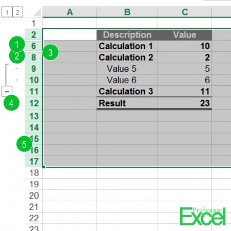
In the screen shot shown below,
- Rows 12 and 13 are hidden
- Formula in cell B2 shows that 2 rows are hidden
- Columns E and F are hidden
- Conditional formatting in cell D1 shows that columns are hidden, to the right of the coloured cell
Get the Hidden Data Warning File
To get the hidden rows and columns warning workbook, go to the Conditional Formatting Examples page on my Contextures site.
In the “Get the Sample Files” section, look for File #3: Hidden Data Warning. The zipped Excel file is in xlsx, and does not contain any macros.

Video: Trouble Unhiding Top Excel Rows
This short video shows you a quick way to see those hidden rows at the top of your Excel worksheet.
________________________
Warning for Hidden Rows and Columns in Excel

________________________
Skip to content
![]()
Let’s assume the following situation: You have received an Excel workbook from a colleague, client or anyone else but you have the feeling, that some rows or columns are hidden. By that, you’ve already done a good job because it is very difficult to spot from the small lines on the side or top that there are hidden rows or columns. But how do you unhide all rows and columns at the same time?
Method 1: Unhide all rows or columns manually
Hide rows and columns
Many people love the “Hide” function for hiding rows or columns, as it is very easy to use: (the numbers are corresponding with the image)
- Mark the row(s) or column(s) that you want to hide.
- Right-click on the row number or column letter and click on “Hide”.
- Unfortunately, it has one big disadvantage: You can hardly recognize hidden rows or columns. It’s only symbolized by a thin double line between the row or column number.
- A better way for hiding rows or columns is the Group function.
Unhide rows and columns
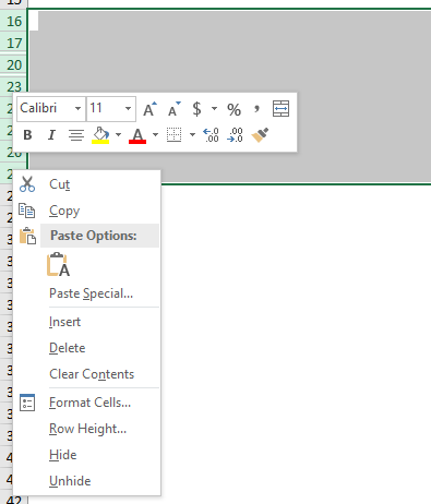
So, how to unhide all hidden rows?
- Select the whole area in which you suspect hidden rows. Alternatively select the whole worksheet in the top left corner.
- >Now double-click on the border between two row numbers (number 5 in the screenshot above). Each row has now it’s minimum size to cover all it’s contents. There is one disadvantage, though: The row height of all selected rows will be reset. So, if you have already set the row heights manually, it will be gone.
- Instead of double-clicking according to the number two above you can right-click on the column or row header (that means the column letter above your hidden column or the row number on the left-hand side). Next, click on “Unhide”.
Method 2: Use Professor Excel Tools
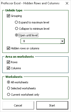
The Excel add-in Professor Excel Tools provide a function for unhiding all hidden rows and columns on all sheets with one click. Alternatively only unhide the rows or columns on the selected or current sheet.
To use the function, click on “Hidden Rows and Columns” in the “Professor Excel” ribbon. Now you’ll see a window as shown on the screenshot on the right-hand side.

This function is included in our Excel Add-In ‘Professor Excel Tools’
(No sign-up, download starts directly)

Henrik Schiffner is a freelance business consultant and software developer. He lives and works in Hamburg, Germany. Besides being an Excel enthusiast he loves photography and sports.
We use cookies on our website to give you the most relevant experience by remembering your preferences and repeat visits. By clicking “Accept”, you consent to the use of ALL the cookies.
.