
Excel for Microsoft 365 Excel for Microsoft 365 for Mac Excel for the web Excel 2021 Excel 2021 for Mac Excel 2019 Excel 2019 for Mac Excel 2016 Excel 2016 for Mac Excel 2013 Excel 2010 Excel 2007 Excel for Mac 2011 Excel Starter 2010 More…Less
This article describes the formula syntax and usage of the COLUMNS
function in Microsoft Excel.
Description
Returns the number of columns in an array or reference.
Syntax
COLUMNS(array)
The COLUMNS function syntax has the following argument:
-
Array Required. An array or array formula, or a reference to a range of cells for which you want the number of columns.
Example
Copy the example data in the following table, and paste it in cell A1 of a new Excel worksheet. For formulas to show results, select them, press F2, and then press Enter. If you need to, you can adjust the column widths to see all the data.
|
Formula |
Description |
Result |
|
=COLUMNS(C1:E4) |
Number of columns in the reference C1:E4. |
3 |
|
=COLUMNS({1,2,3;4,5,6}) |
Number of columns in the array constant {1,2,3;4,5,6}. There are two 3-column rows, containing 1,2, and 3 in the first row and 4,5, and 6 in the second row. |
3 |
Need more help?
Want more options?
Explore subscription benefits, browse training courses, learn how to secure your device, and more.
Communities help you ask and answer questions, give feedback, and hear from experts with rich knowledge.
The COLUMNS function is a built-in function in Microsoft Excel. It falls under the category of LOOKUP functions in Excel. The COLUMNS function returns the total number of columns in the given array or collection of references. The purpose of the COLUMNS formula in Excel is to know the number of columns in an array of references.
For example, the formula =COLUMNS(A1:E3) will return as 5 since the range A1:E3 has 5 columns, A, B, C, D, and E, respectively.
Table of Contents
- What Is COLUMNS Function In Excel?
- Syntax
- How To Use COLUMNS Formula In Excel?
- Examples
- Important Things To Note
- Frequently Asked Questions
- Columns Function in Excel Video
- Recommended Articles
- The COLUMNS function in excel is used to find the number of columns used in the worksheet.
- The formula of the columns function in excel is =COLUMN(array), where the array is the only mandatory argument.
- The array shows the range of cells for which the number of columns is derived.
- We can choose either a single cell or a range as the value in the array argument.
- It is important to know that the function will return only the number of columns even if the chosen array has multiple rows and columns.
Syntax
- array = This is a required parameter. An array / a formula resulting in an array / a reference to a range of Excel cells for which the number of columns is to be calculated.
The COLUMNS function has only one argument, and it is mandatory.
How To Use COLUMNS Formula In Excel?
You can download this COLUMNS Function Excel Template here – COLUMNS Function Excel Template
The said function is a worksheet (WS) function. As a WS function, columns can be inserted as a part of the formula in a worksheet cell.
Let us look at the examples given below to understand the use of the COLUMNS function in excel.
Examples
Example #1 – Total Columns In A Range
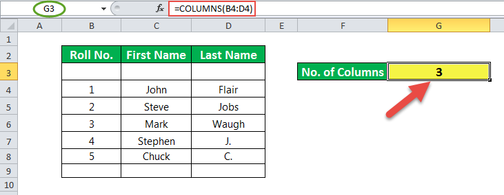
In the example of this column, cell G3 has a formula associated with it. So, G3 is a result cell.
The argument for the COLUMNS function in excel is a cell range, which is B4:D4. Here, B4 is a starting cell, and D4 is the ending cell.
The number of columns between these two cells is 3. So, the result is 3.
Example #2 – Total Cells In A Range

In this example, cell G4 has a formula associated with it. So, G4 is a result cell.
The formula is COLUMNS (B4: E8) * ROWS*B4: E8). Then, multiplication is performed between the total number of columns and a total number of rows for the given range of cells in the sheet.
Here, the total number of columns is four, and the total number of rows is 5. So, the total number of cells is 4*5 = 20.
Example #3 – Get The Address Of The First Cell In A Range

Here, the dataset is named data. Further, this data is used in the formula.
You may refer to the steps given below to name the dataset.
- Step 1: Select the cells.
- Step 2: Right-click and choose Define Name.
- Step 3: Name the dataset as data.

In the example of these columns, cell G6 has a formula associated with it. So, G6 is a result cell. The formula is to calculate the first cell in the dataset represented by the name data. The result is $B$4, i.e., B4, the last cell in the selected dataset.
The formula uses the ADDRESSES function, which has two parameters: row number and column number.
E.g., ADDRESS (8,5) returns $B$4. Here, 4 is the row number, and 2 is the column number. So, the function returns a cell denoted by these row and column numbers.
Here, a row number is calculated by
ROW(data)
And the column number is calculated by
COLUMN(data)
Example 4 – Get The Address Of The Last Cell In A Range

Here, the dataset is named data. Further, this data is used in the column’s formula in Excel. We can refer to the steps given below to name the dataset.
- Step 1: Select the cells.
- Step 2: Right-click and choose Define Name.
- Step 3: Name the dataset as data.

In this COLUMNS example, cell G5 has a formula associated with it. So, G5 is a result cell. The formula is to calculate the last cell in the dataset represented by the name data. The result is $E$8, i.e., E8, the last cell in the selected dataset.
The formula uses the ADDRESSES function, which has two parameters: row number and column number.
E.g., ADDRESS (8,5) returns $E$8. Here, 8 is the row number, and 5 is the column number. So, the function returns a cell denoted by these row and column numbers.
Here, the row number is calculated by
ROW(data)+ROWS(data-1)
And the column number is calculated by
COLUMN(data)+COLUMNS(data-1)
Important Things To Note
- The argument of the COLUMNS function in Excel can be a single cell address or a range of cells.
- The argument of the COLUMNS function cannot point to multiple references or cell addresses.
Frequently Asked Questions
1) What is the columns function in excel?
Columns Function in excel is a built-in excel function used to derive the number of columns used in the worksheet. The syntax of the COLUMNS function in excel is =COLUMNS(array). For example, consider the table with details of 3 employees.
We can calculate the number of columns used in the data using the columns function in excel.
Step 2: Select the range A1:C4 as shown in the below image.
Step 3: Press Enter key
We will get the result as shown in the below image.
2) When can we use the columns function in excel?
Columns Function in excel is used when we have to find the number of columns used in the data. Especially while working with large datasets, this function will be useful.
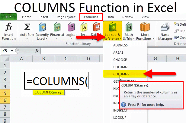
3) How to insert columns function in excel?
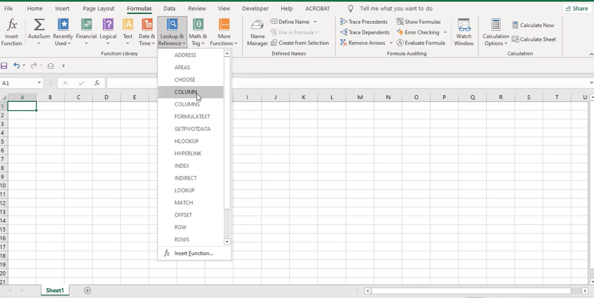
We can insert columns function in excel by selecting Formulas > Lookup & Reference in the Function Library group > COLUMNS function.
Alternatively, we can also type =COLUMNS and choose the cell array.
Columns Function in Excel Video
Recommended Articles
This article is a guide to Columns Function in Excel. We discuss the columns formula in Excel and how to use it, along with examples and downloadable templates. You can also go through our other suggested articles: –
- Excel Column Lock
- Excel Freeze Columns
- Group Column in Excel
- Column in Excel
- Break Links in Excel
COLUMNS in Excel (Table of Contents)
- COLUMNS in Excel
- How to Use COLUMNS Function in Excel?
COLUMNS in Excel
The columns function in excel is another easiest function to apply, which simply counts the number of columns that are selected. It returns the count of the number of columns selected in the array. For this, we just have to select the complete columns or columns in the form of a table or matrix. It will simply return the count of columns there in an array.
COLUMNS Formula in Excel:
The Formula for the COLUMNS Function in Excel is as follows:
The COLUMNS Function formula has a below-mentioned argument:
Array: reference to an array OR range of cells for which we have to calculate a number of columns.
Note:
- If the range of cells or array contains multiple rows and columns, only the columns are counted.
- COLUMNS Function in Excel will always return a positive numeric value.
How to Use COLUMNS Function in Excel?
This COLUMNS Function is very simple easy to use. Let us now see how to use the COLUMNS Function in Excel with the help of some examples.
You can download this COLUMNS Function Excel Template here – COLUMNS Function Excel Template
Example #1
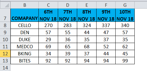
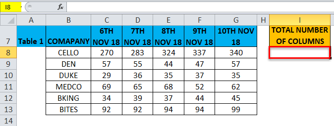
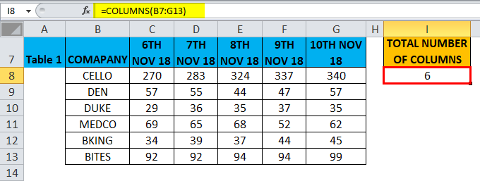
In the below-mentioned example, I have a dataset in a range, i.e. B7:G13, where it contains the company & its share value on a daily basis. Here I need to find out the number of columns in that range with the help of the COLUMNS Function.
Let’s apply the COLUMNS function in cell “I8”.
Select the cell “I8” where the COLUMNS function needs to be applied, Click the insert function button (fx) under the formula toolbar, a dialog box will appear, type the keyword “COLUMNS” in the search for a function box, COLUMNS function will appear in select a function box.
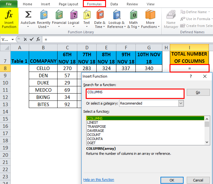
Double click on COLUMNS function, a dialog box appears where arguments for COLUMN function needs to be filled or entered, i.e. =COLUMNS (array)
Array: Reference to an array OR range of cells for which we have to calculate a number of columns, i.e. Here it is B7:G13, where Here, B7 is a starting cell and G13 is the ending cell in a table or range.
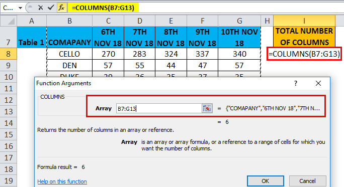
Click ok after entering the arguments in the COLUMNS function. i.e.=COLUMNS (B7:G13) COLUMNS function calculates the total number of columns present in a range, i.e. 6. The number of columns in between these two cells (B7 & G13) is 6; hence it results in 6.
Example #2
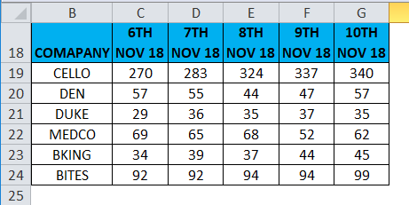
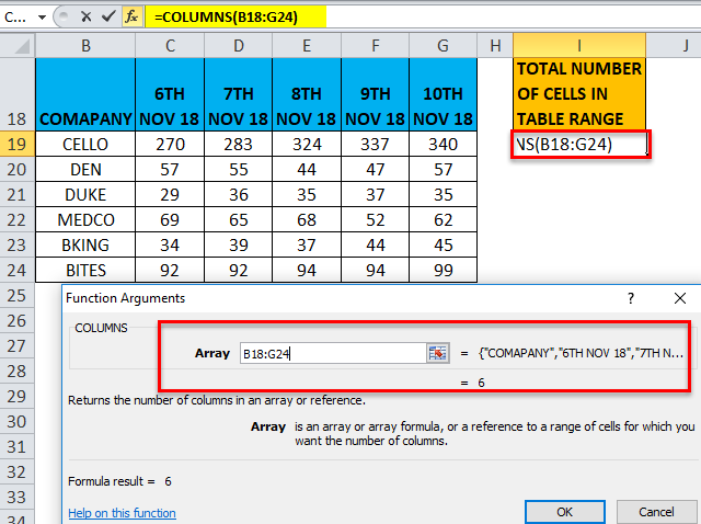
In the below-mentioned example, I have a dataset in a range, i.e. B18:G24, where it contains the company & its share value on a daily basis. Here I need to find out the Total cell in range with the help of the COLUMNS function.
Let’s apply the COLUMNS function in cell “I19”.
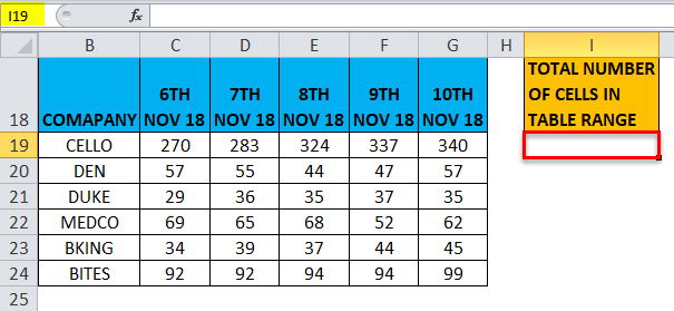
Select the cell “I19” where the COLUMNS function needs to be applied, Click the insert function button (fx) under the formula toolbar, a dialog box will appear, type the keyword “COLUMNS” in the search for a function box, COLUMNS function will appear in select a function box.
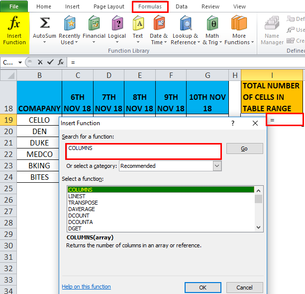
Double click on COLUMNS function, A dialog box appears where arguments for COLUMN function needs to be filled or entered i.e.
=COLUMNS (array)
Array: reference to an array OR range of cells for which we have to calculate a number of columns, i.e. Here it is B18:G24 where Here, B18 is a starting cell and G24 is the ending cell in a table or range.
Multiplication needs to be performed between the total number of columns and a total number of rows for the given array or range of cells to get the total number of cells in an array or table.
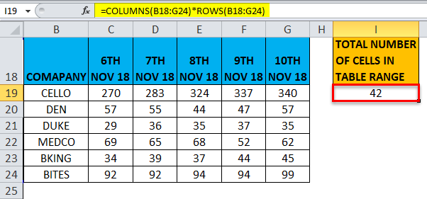
i.e. =COLUMNS(B18:G24)*ROWS(B18:G24)
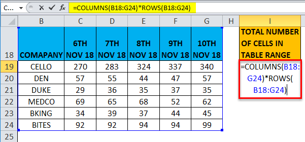
Here, the total number of rows is 7 & the total number of columns is 6. So, the total number of cells is 7*6 = 42
Example #3
The COLUMNS function is important when using functions where a column argument is required, e.g. VLOOKUP in case of a huge number of datasets; it is not easy to manually count the number of columns in a table array.
During these scenarios, In the VLOOKUP function, The COLUMNS function is used to return the col_index_num argument value.
Let check out the difference between the Vlookup function with & without Columns Function.
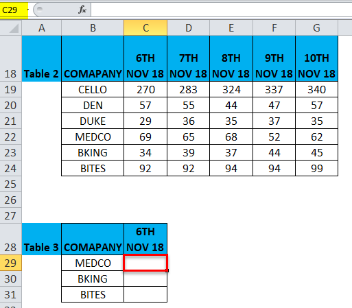
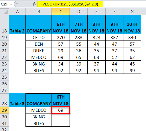
In the below-mentioned example, table2 contains the company in column B & its share value on a daily basis ( 6th, 7th,8th, 9th & 10thNov 2018) in columns C, D, E, F & G, respectively.
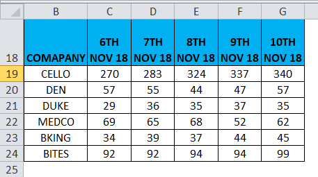
Table 3 contains the company name in column B; our objective here in this table is to find out its share value on 6th Nov 2018 in column C, with the help of table 2 reference by using the VLOOKUP function.
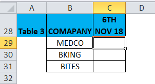
Prior to applying the VLOOKUP formula, you should be aware of it. Vertical lookup or VLOOKUP references vertically aligned tables and quickly finds data in relation to the value the user enters.
VLOOKUP Function without COLUMNs Function
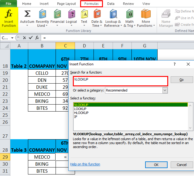
Let’s apply the VLOOKUP function in cell “C29”.
Select the cell “C29”. where the VLOOKUP function needs to be applied; click the insert function button (fx) under the formula toolbar, a dialog box will appear, type the keyword “VLOOKUP” in the search for a function box, VLOOKUP function will appear in select a function box.
Double click on the VLOOKUP function, A dialog box appears where arguments for the VLOOKUP function need to be filled or entered.
The Formula for the VLOOKUP function is:
VLOOKUP (lookup_value, table_array, col_index_num, [range_lookup])
- lookup_value: The value you want to look up, i.e. “B29” or “MEDICO.”
- table_array: Range where the lookup value is located, i.e. select table 2 range B18:G24 & click function f4 key to lock a range, i.e. $B$18:$G$24.
- col_index_num: column number in a table array from which the matching value should be returned. Here the company share value on 6th November 2018 is in table 2 & it is in the second column, i.e. 2
- range_lookup: FALSE for an exact match or TRUE for an approximate match. Select 0 or false.
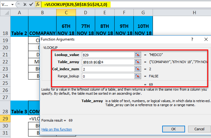
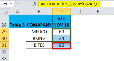
=VLOOKUP(B29,$B$18:$G$24,2,0) returns the share value of Medco on 6th November 2018, i.e. 69
To get the finalized data for other company share prices, click inside cell C29 and you’ll see the cell selected, then Select the cells till C31. So that column range will get selected, once it got selected, click on Ctrl + D so that the VLOOKUP formula is applied to a whole range.
VLOOKUP Function with COLUMNS Function
Above the table 2 column header, B17 to G17 is the column number that needs to be mentioned prior to applying Vlookup with the columns function.
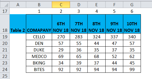
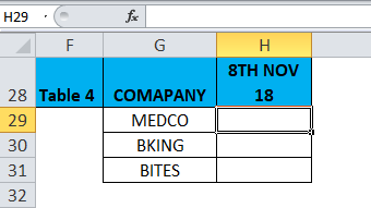
Table 4 contains the company name in column G; our objective here in this table is to find out its share value on 8th Nov 2018 in column H, with the help of table 2 reference by using VLOOK with COLUMNS function.
In VLOOKUP Function without COLUMNS Function, Formula was:
=VLOOKUP(C29,$B$18:$G$24,2,0)
Where 2 was the column index number, here let’s replace this with the COLUMNS($B$17:$E$17) function in the Vlookup function in cell H29 of table 4. Here we need a share price value for 8th Nov 18, hence the select column reference B17 to E17 in columns function of the table.
i.e. =VLOOKUP(G29,$B$18:$G$24,COLUMNS($B$17:$E$17),0)
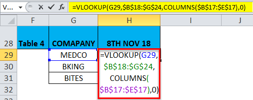
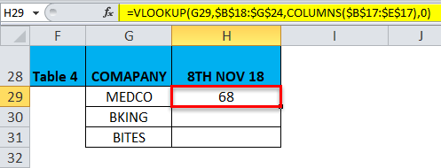
=VLOOKUP(G29,$B$18:$G$24, COLUMNS($B$17:$E$17),0) returns the share value of Medco on 8th November 2018, i.e. 68
To get the finalized data for other company share prices, click inside cell H29 and you’ll see the cell selected, then Select the cells till H31. So that column range will get selected, once it is selected, press Ctrl + D so that the formula is applied to a whole range.
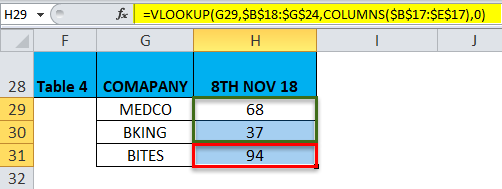
Here simultaneously, we have to change the column reference in column function & lookup value based on the data requirement.
Things to Remember
- The COLUMNS Function in Excel is important or significant when using functions where a column argument is required (e.g. VLOOKUP); in the case of a huge number of datasets, it is not an easy task to manually count the number of columns in a table array (Explained in example 3).
- The array argument in the COLUMNS Function can be either a range of cells or single-cell addresses.
- If the range of cells or array contains multiple rows and columns, only the columns are counted.
- COLUMNS function in Excel will always return a positive numeric value.
Recommended Articles
This has been a guide to COLUMNS in Excel. Here we discuss the COLUMNS Formula in Excel and how to use COLUMNS Function in Excel along with excel examples and downloadable excel templates. You may also look at these useful functions in excel –
- Freeze Columns in Excel
- Column Header in Excel
- COLUMNS Formula in Excel
- VBA Columns
Excel COLUMNS Function (Example + Video)

When to use Excel COLUMNS Function
Excel COLUMNS function can be used when you want to get the number of columns in a specified range or array.
What it Returns
It returns a number that represents the total number of columns in the specified range or array.
Syntax
=COLUMNS(array)
Input Arguments
- array – it could be an array, an array formula or a reference to a contiguous range of cells.
Additional Notes
- Even if the array contains multiple rows and columns, only the columns are counted. For example:
-
COLUMNS(A1:B1) returns 2.
-
COLUMNS(A1:B100) also returns 2.
-
- This formula can be useful when you want to get a sequence of numbers as you go to the right in your worksheet.
- For example, if you want 1 in A1, 2 in B1, 3 in C1 and so on, use the following formula =COLUMNS($A$1:A1). As you would drag this to the right, the reference inside it would change and the number of columns in the reference would get incremented by one. For example, when you drag it to column B1, the formula becomes COLUMNS($A$1:B1) which then returns 2.
Excel COLUMNS Function – Examples
Here are two examples of using the Excel COLUMNS function.
Example 1: Finding the number of Columns in an Array

In the example above, =COLUMNS(A1:A1) returns 1 as it covers one row (which is A1). Similarly, =COLUMNS(A1:C1) returns 3 as the array A1:C1 covers four columns in it.
Also, note that it only counts the number of columns. Hence, whether the array is A1:C1, or A1:C5, it would return 3 in both the cases.
Example 2: Getting a Sequence of Numbers in a Column

Excel COLUMNS function can be used to get a sequence of numbers. Since the first reference is fixed, as you copy the formula down, the second reference changes and so does the row numbers in the array.
Excel COLUMNS Function – Video Tutorial
Related Excel Functions:
- Excel COLUMN Function.
- Excel ROW Function.
- Excel ROWS Function
Other articles you may also like:
- Row vs Column in Excel – What’s the Difference?
In this article, we are going to see the details about Excel ROW, ROWS, COLUMN, COLUMNS functions, and their usages.
ROW Function
The ROW( ) function basically returns the row number for a reference.
Syntax:
=ROW([reference])
Example :
=ROW(G100); Returns 100 as output
as G100 is in the 100th row in the Excel sheet
If we write no argument inside the ROW( ) it will return the row number of the cell in which we have written the formula.
Here the following returns are achieved:
=ROW(A67) // Returns 67
=ROW(B4:H7) // Returns 4
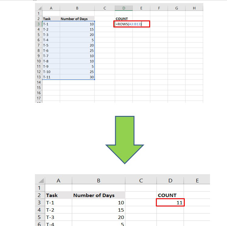
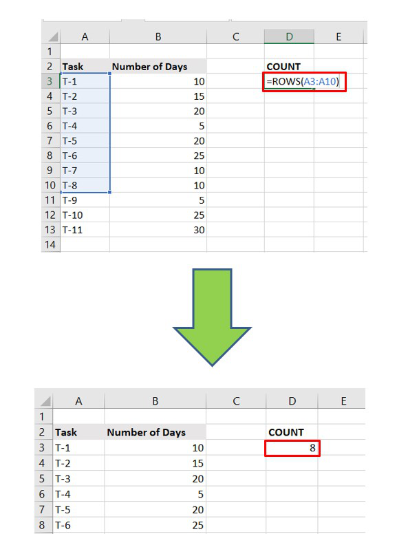
ROWS Function
It is the extended version of the ROW function. ROWS function is used to return the number of rows in a cell range.
Syntax:
=ROWS([array])
Example :
=ROWS(A2:A11) // Returns 10 as there are ten rows
It is important to note that writing the column name is trivial here. We can also write :
=ROWS(2:13) // Returns 12
COLUMN Function
The column function usually returns the column number of a reference. There are 16,384 columns in Excel from the 2007 version. It returns the value 1 to 16,384.
Syntax:
=COLUMN([reference])
Example :
=COLUMN(E20) // Returns 5 as output
as E is the fifth column in the Excel sheet
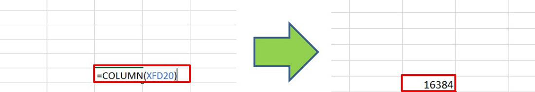
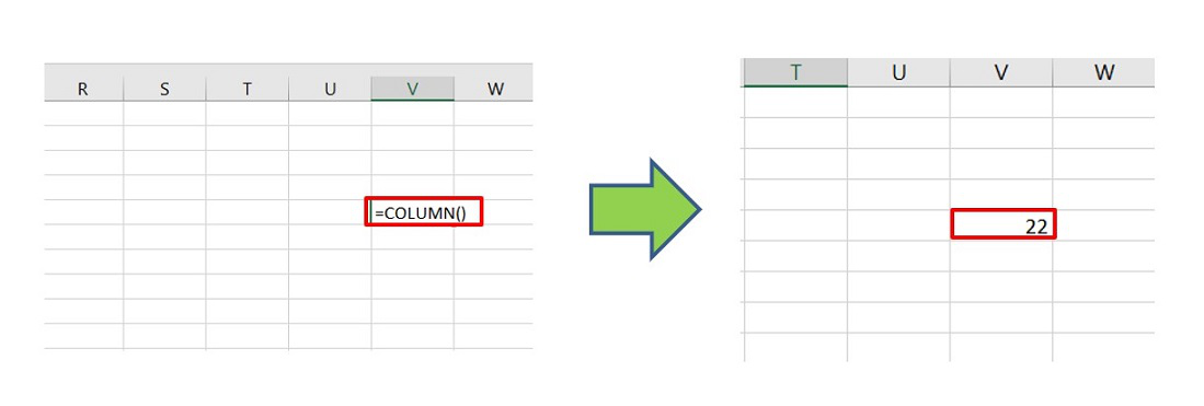
Last Column of Excel
Similar to the ROW function, the argument is not mandatory. If we don’t write any argument, it will return the index of the column in which the formula is written.
COLUMNS Function
It is the extended version of the COLUMN( ). It returns the number of columns for a given cell range.
Syntax:
=COLUMNS([array])
Example :
=COLUMNS(B12:E12) // Returns 4 as output as
there are 4 columns in the given range
It is important to note that writing the row number is trivial here. We can also write :
=COLUMNS(B:E) // Returns 4
ROWS And COLUMNS Functions in Array Formulas
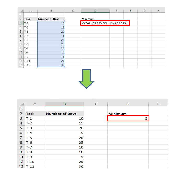
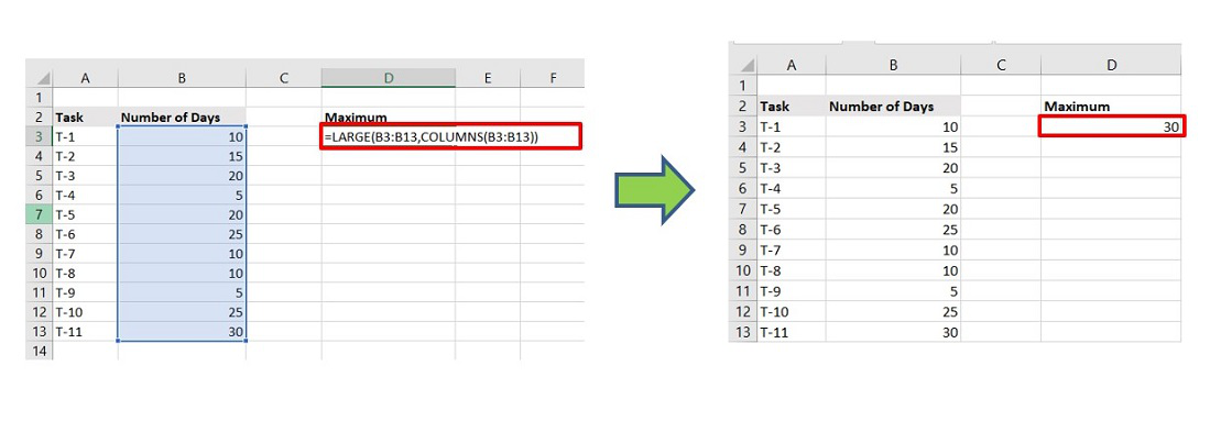
We can use the ROWS( ) and COLUMNS( ) in array formulas using SMALL( ), LARGE( ), VLOOKUP( ) functions in Excel.
Example :
The smallest value is returned to the provided cell range.
The largest value is returned to the provided cell range.
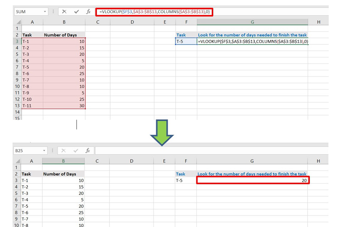
Say, we need to find the number of days needed to complete Task number 5.
The steps are :
Step 1: Choose any cell and write the name of the Task.
Step 2: Beside that cell write the “Formula” as shown below to get the “Number of Days” need :
=VLOOKUP($F$3,$A$3:$B$13,COLUMNS($A$3:$B$13),0)
F3 : Reference of the Task T-5
A3:B13 : Cell range of the entire table for VLOOKUP to search
Step 3: Click Enter.
Now, it can be observed it returns 20 as output which is perfect as per the data set.
Functions are an important part of Excel and assist in calculating many data for many users. Column functions and Columns functions are Lookup and Reference functions in Microsoft Excel.
The Column function returns the column number of a reference, and its formula is Column([reference]).
The syntax for the Column function is:
Column
Reference: The cell or range of cells or range of cells for which you want to return the column number. It is optional.
The Columns function returns the number of columns in a reference, and its formula is Columns(array).
The syntax for the Columns function is:
Columns
Array: An array or array formula, or a reference to a range of cells for which you want the number of columns. It is required.
Launch Microsoft Excel.

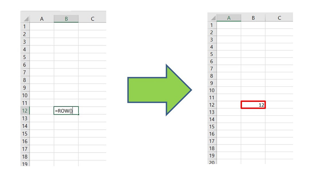
Type into the cell A1, =Column().
Then press Enter.
You will notice that the cell will return the cell number of the cell that contains the formula.
 (How to use the Column function in Excel)")
Type into any of the cells in your spreadsheet =Column(D4).
Then press Enter, and the result would be 4 because the D column number is 4.
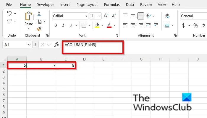
Type into any of the cells in your spreadsheet =Column(=COLUMN(F1:H5).
Then press Enter, and the result would be 6,7, and 8.
There are two other methods to use the Column function.
Method one is to click the fx button on the top left of the Excel worksheet.
An Insert Function dialog box will appear.
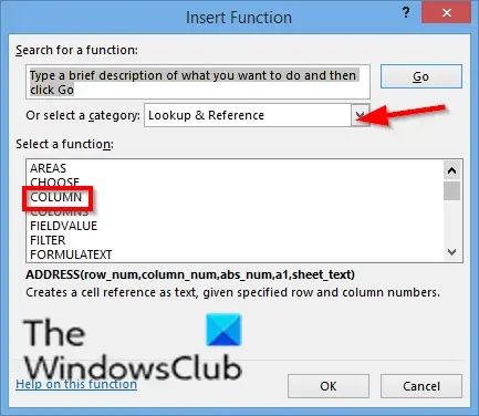
Inside the dialog box, in the section Select a Category, select Lookup and Reference from the list box.
In the section Select a Function, choose the Column function from the list.
Then click OK.
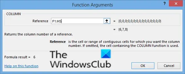
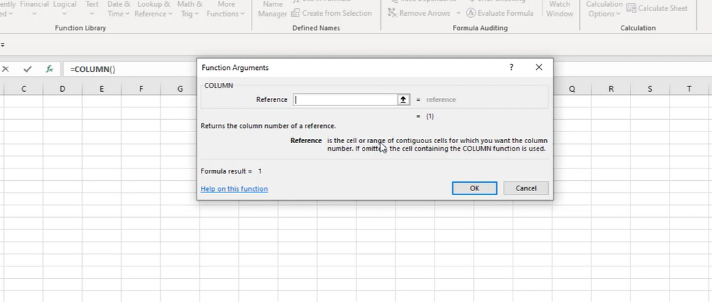
A Function Arguments dialog box will open.
In the Reference entry box, type cell F1:H5.
Then click OK.
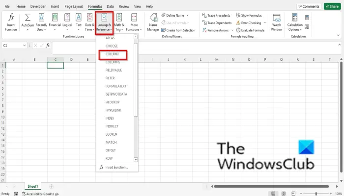
Method two is to click the Formulas tab and click the Lookup and Reference button in the Function Library group.
Then select Column from the drop-down menu.
A Function Arguments dialog box will open.
Follow the same method in Method 1.
Then click Ok.
How to use the Excel Columns function
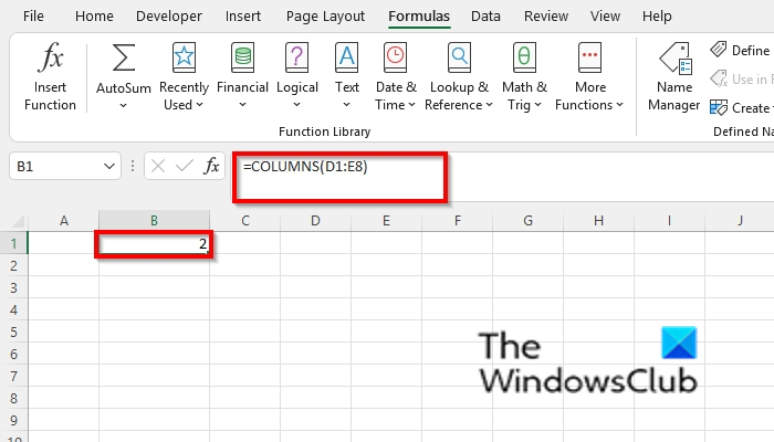
Type into any of the cells =COLUMNS(D1:E8).
Then press Enter.
The result is 2 because it is the number of columns in the reference.
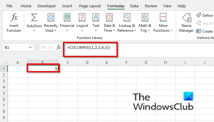
Type into any of the cells in your spreadsheet =COLUMNS({1,2,3,4,5}).
Then press Enter, and the result would be 5 because it gives the column count for an array constant.
There are two other methods to use the Columns function.
Method one is to click the fx button on the top left of the Excel worksheet.
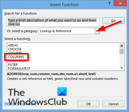
An Insert Function dialog box will appear.
Inside the dialog box, in the section Select a Category, select Lookup and Reference from the list box.
In the section Select a Function, choose the Columns function from the list.
Then click OK.
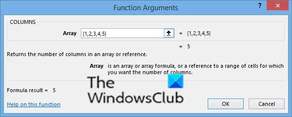
A Function Arguments dialog box will open.
In the Reference entry box, type cell {1,2,,4,5}.
Then click OK.
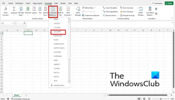
Method two is to click the Formulas tab and click the Lookup and Reference button in the Function Library group.
Then select Columns from the drop-down menu.
A Function Arguments dialog box will open.
Follow the same method in Method 1.
Then click Ok.
READ: How to use the PROPER function in Excel
What is Column in Excel?
In Microsoft Excel, a column runs horizontally and is in as an Alphabetical letter header on the top of the spreadsheet. Excel spreadsheet can have 16,384 columns in total. The data goes from up and down.
READ: How to use the SUMSQ function in Excel
How do I write in a Column in Excel?
If you want to insert a column in Excel, click the column and click insert in the context menu. A column will appear. To type under the column header, click in the row under the column and type your data.
We hope this tutorial helps you understand how to use the Column and Columns function in Microsoft Excel; if you have questions about the tutorial, let us know in the comments.
In this article, we will discuss the “Columns Function” in Excel and “how to apply a function to a column in Excel”, a useful tool that allows you to manipulate data in various ways. Microsoft Excel is a powerful tool millions worldwide use to manage, analyze and interpret data. One of its most powerful features is the Columns Function, which allows users to manipulate data in many ways. This function can be used to perform a variety of tasks, from sorting and filtering data to calculating totals and averages.
You’ve come to the right place if you’re new to Excel or want to learn more about using the Columns Function effectively. In this guide, we’ll explore everything you need to know to master this powerful tool, including tips, tricks, and common pitfalls to avoid. As a business owner or data analyst, you know how important it is to have accurate and organized data. Excel’s Columns function is a powerful tool to help you achieve this goal. In this article, we will dive into the details of the Columns function and show you how to use it to optimize your data analysis.
In this article, we will provide you with a detailed guide on using the Columns Function in Excel, including examples of how it can be used to manipulate data.
How to Use the Columns Function?
You have a column in your Excel spreadsheet containing a first and last name, separated by a space. You can use the Columns function to split this column into two separate columns, one for the first name and one for the last name.
To do this, follow these steps:
- Select the column you want to split.
- Click on the Data tab and the Text to Columns button.
- In the Convert Text to Columns Wizard, select the Delimited option and click Next.
- Choose the delimiter that separates the first and last name (in this case, a space) and click Next.
- Choose the format of the destination columns (General, Text, Date, etc.) and click Finish.
Your column will now be split into two separate columns, one for the first name and one for the last name. This can be incredibly useful when working with large data sets that need to be organized or when importing data from an external source that needs manipulation.
As businesses rely on data for decision-making, Microsoft Excel remains a popular tool for organizing, analyzing, and visualizing data. One of the powerful features of Excel is its ability to apply functions to columns, which enables users to perform complex calculations on large data sets quickly and efficiently. In this article, we will explore the various ways to apply a function to a column in Excel and provide tips and tricks to make the process easier and more effective.
COLUMNS Formula in Excel
Benefits of Using the Columns Function
Using the Columns function in Excel can benefit your data analysis. Here are just a few:
- Saves Time: Using the Columns function, you can quickly split large data sets into smaller, more manageable pieces. This can save you significant time when working with large amounts of data.
- Organizes Data: The Columns function can help you organize your data by splitting it into more manageable columns. This can make it easier to analyze and work with your data.
- Improves Accuracy: Splitting your data into smaller columns can improve accuracy by making it easier to identify errors or inconsistencies in your data.
- Enables Manipulation: The Columns function allows you to manipulate your data in ways that would not be possible without splitting it into smaller columns. This can help you perform more complex data analysis tasks.
- Increases Flexibility: By splitting your data into smaller columns, you can increase the flexibility of your data analysis. This can allow you to perform more complex tasks and gain deeper insights into your data.
COLUMNS Formula in Excel
Examples of Using the Columns Function:
To help illustrate how the Columns Function can be used, we will provide a few examples:
Example 1: Finding the Total Revenue for a Sales Report
Suppose you have a sales report in Excel that contains several columns, including “Product Name,” “Price,” and “Units Sold.” You want to find the total revenue for the report by multiplying the “Price” and “Units Sold” columns and then summing the results.
You would first select the “Price” and “Units Sold” columns to do this. Then, apply the following formula to the selected columns: =SUM(B2:B10*C2:C10). This would multiply the values in the “Price” and “Units Sold” columns for each row and then sum the results to give you the total revenue for the report.
Example 2: Filtering Data Based on a Specific Criteria
Suppose you have a large data set in Excel that contains several columns, including “Product Name,” “Price,” and “Category.” You want to filter the data only to show products that belong to a specific category.
To do this, you would first select the entire data set. Then, go to the “Data” tab in the Excel ribbon and click on the “Filter” button. This would add a filter to each column in your data set. Next, you would click on the filter drop-down in the “Category” column and select the specific category that you want to filter by. This would update the data set only to show products that belong to the selected category.
In conclusion, the Columns Function in Excel is a powerful tool that can manipulate data in various ways. Selecting a range of columns and applying a specific function allows you to quickly sort, filter, and analyze your data. We hope this article has provided you with a comprehensive guide on how to use the Columns Function in Excel, and we encourage you to start using this feature to enhance your productivity and efficiency in Excel.
Top 5 Best Ways to Apply a Function to a Column in Excel
What is a Function in Excel? In Excel, a function is a predefined formula that performs a specific calculation, such as adding, subtracting, or averaging values in a range of cells. Functions can take arguments, which are values or cell references that the function uses to calculate. Excel has a wide range of functions organized into categories such as Math & Trig, Date & Time, and Statistical.
Applying a Function to a Column Using AutoSum
One of the easiest ways to apply a function to a column in Excel is to use the AutoSum feature. AutoSum is a built-in tool that automatically detects the range of data and applies the appropriate function to the selected column. To use AutoSum, click on an empty cell below the column of data and click on the AutoSum button in the Editing group of the Home tab. Excel will automatically select the column of data and insert the SUM function.
Using the Function Wizard to Apply a Function to a Column Excel’s Function
Wizard provides a powerful tool for applying functions to columns of data. The Function Wizard allows users to browse through Excel’s extensive library of functions, select the desired function, and specify the range of data to which the function should be applied. To access the Function Wizard, click on the fx button next to the formula bar. Also, the Function Wizard will open, and users can select the desired function and specify the range of data.
Using Absolute References to Apply a Function to Multiple Columns
When applying a function to multiple columns of data, it can be helpful to use absolute references. Absolute references are cell references that do not change when copied or filled, allowing users to apply a function to multiple columns of data with ease. To use absolute references, simply add a dollar sign ($) before the column and row reference in the function. For example, =$A$1+$B$1 would add the values in cells A1 and B1 and remain unchanged when copied or filled.
Using the Fill Handle to Apply a Function to a Column Excel’s
Fill Handle is a powerful tool for applying functions to columns of data quickly and easily. The Fill Handle allows users to drag the selection to adjacent cells, automatically filling the formula down the column. Also, to use the Fill Handle, select the cell containing the formula and click and drag the small square in the bottom right corner of the cell to the desired range of cells.
Using Array Formulas to Apply a Function to a Column
Array formulas are a powerful tool for complex calculations on large data sets. Array formulas allow users to apply a function to an entire column of data with a single formula, making it a powerful tool for analyzing data. Also, to use array formulas, enter the formula using curly braces ({}) and press Ctrl + Shift + Enter to apply the formula to the entire column.
Conclusion
The Columns function in Excel is a powerful tool that can help you optimize your data analysis. Using this function, you can quickly and easily split large data sets into smaller, more manageable pieces. This can save you time, improve accuracy, and enable more complex data analysis tasks. If you want to learn more about using Excel to optimize your data analysis, check out our blog for helpful tips and tricks.

I am studying at Middle East Technical University. I am interested in computer science, architecture, physics and philosophy.
Love,
Cansu
Tags: #ExcelCharts #ExcelDashboard #ExcelFormulas #ExcelFunctions #ExcelTemplates #ExcelTipsAndTricks #ExcelTutorials
Summary
The Excel COLUMNS function returns the count of columns in a given reference. For example, COLUMNS(A1:C3) returns 3, since the range A1:C3 contains 3 columns.
Purpose
Get the number of columns in an array or reference.
Return value
Arguments
- array — A reference to a range of cells.
Syntax
Usage notes
The COLUMNS function returns the count of columns in a given reference as a number. For example, COLUMNS(A1:C3) returns 3, since the range A1:C3 contains 3 columns. COLUMNS takes just one argument, called array, which should be a range or array.
Examples
Use the COLUMNS function to get the column count for a given reference or range. For example, there are 6 columns in the range A1:F1 so the formula below returns 6:
=COLUMNS(A1:F1) // returns 6
The range A1:Z100 contains 26 columns, so the formula below returns 100:
=COLUMNS(A1:Z100) // returns 26
You can also use the COLUMNS function to get a column count for an array constant:
=COLUMNS({1,2,3,4,5}) // returns 5
Although there is no built-in function to count the number of cells in a range, you can use the COLUMNS function together with the ROWS function like this:
=COLUMNS(range)*ROWS(range) // total cells
=COLUMNS(A1:Z100)*ROWS(A1:Z100) // returns 2600
More details here.
Notes
- Array can be a range or a reference to a single contiguous group of cells.
- Array can be an array constant or an array created by another formula.
- To count rows, see the ROW function.
- To get column numbers, see the COLUMN function.
- To lookup a column number, see the MATCH function.

Author![]()
Dave Bruns
Hi — I’m Dave Bruns, and I run Exceljet with my wife, Lisa. Our goal is to help you work faster in Excel. We create short videos, and clear examples of formulas, functions, pivot tables, conditional formatting, and charts.