
If you have a worksheet with data in columns that you need to rotate to rearrange it in rows, use the Transpose feature. With it, you can quickly switch data from columns to rows, or vice versa.
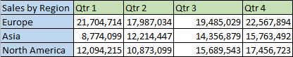
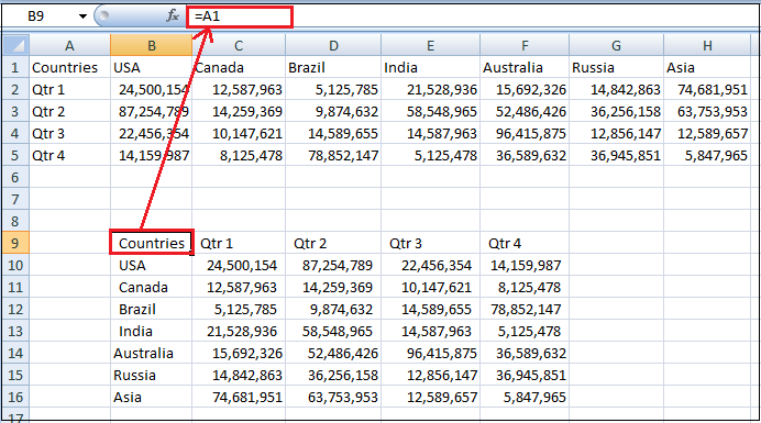
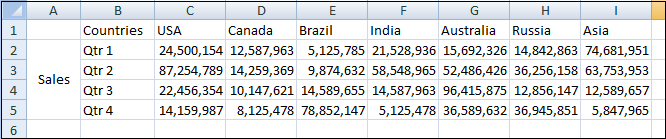
For example, if your data looks like this, with Sales Regions in the column headings and and Quarters along the left side:
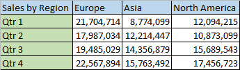
The Transpose feature will rearrange the table such that the Quarters are showing in the column headings and the Sales Regions can be seen on the left, like this:
Note: If your data is in an Excel table, the Transpose feature won’t be available. You can convert the table to a range first, or you can use the TRANSPOSE function to rotate the rows and columns.
Here’s how to do it:
-
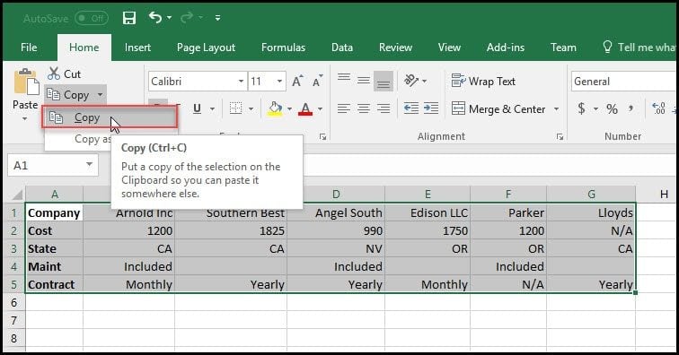
Select the range of data you want to rearrange, including any row or column labels, and press Ctrl+C.
Note: Ensure that you copy the data to do this, since using the Cut command or Ctrl+X won’t work.
-
Choose a new location in the worksheet where you want to paste the transposed table, ensuring that there is plenty of room to paste your data. The new table that you paste there will entirely overwrite any data / formatting that’s already there.
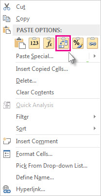
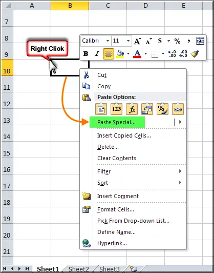
Right-click over the top-left cell of where you want to paste the transposed table, then choose Transpose
 .
.
-
After rotating the data successfully, you can delete the original table and the data in the new table will remain intact.
 .
.
Tips for transposing your data
-
If your data includes formulas, Excel automatically updates them to match the new placement. Verify these formulas use absolute references—if they don’t, you can switch between relative, absolute, and mixed references before you rotate the data.
-
If you want to rotate your data frequently to view it from different angles, consider creating a PivotTable so that you can quickly pivot your data by dragging fields from the Rows area to the Columns area (or vice versa) in the PivotTable Field List.
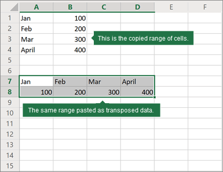
You can paste data as transposed data within your workbook. Transpose reorients the content of copied cells when pasting. Data in rows is pasted into columns and vice versa.
Here’s how you can transpose cell content:
-
Copy the cell range.
-
Select the empty cells where you want to paste the transposed data.
-
On the Home tab, click the Paste icon, and select Paste Transpose.
Excel Columns to Rows (Table of Contents)
- Columns to Rows in Excel
- How to Convert Columns to Rows in Excel using Transpose?
Columns to Rows in Excel
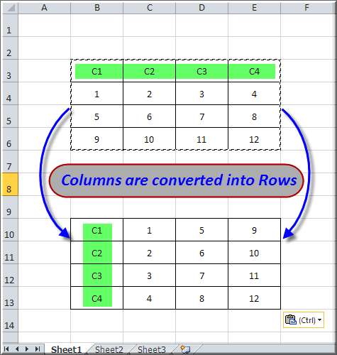
In Excel, to convert any Columns to Rows, first select the column which you want to switch and copy the selected cells or columns. To proceed further, go to the cell where you want to paste the data. Then from the Paste option, which is under the Home menu tab, select the Transpose option. This will convert the selected Columns into Rows. You can also use the shortcut keys Alt + H + V + T, which will directly take us to the TRANSPOSE function.
Paste Special Option.
The shortcut key for paste special:
Once you have copied the range of cells that need to be transposed, click on Alt + E + S in a cell where you want to paste special a dialog box popup window with the transpose option.
How to Convert Columns to Rows in Excel using Transpose?
Converting data from column to row in excel is very simple and easy. Let’s understand the working of converting columns to rows by using some examples.
You can download this Convert Columns to Rows Excel Template here – Convert Columns to Rows Excel Template
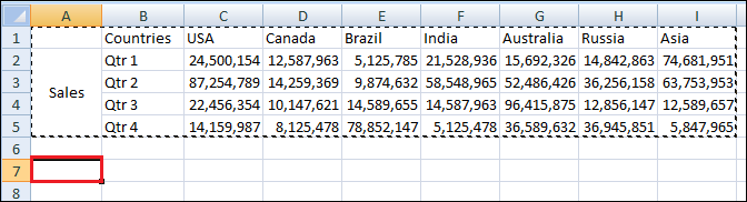
Example #1
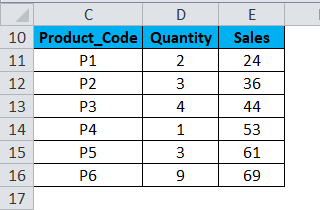
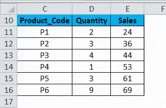
The below-mentioned Pharma sales table contains the medicine product code in column C (C10 to C16), quantity sold in column D (D10 to D16) & total sales value in column E (E10 to E16).
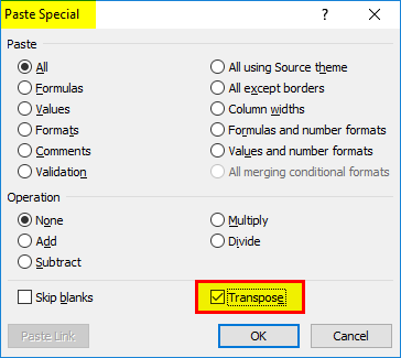
Here we need to convert its orientation from columns to rows with the help of a paste special option in excel.
- Select the whole table range, i.e. all the cells with the dataset in a spreadsheet.
- Copy the selected cells by pressing Ctrl + C.
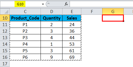
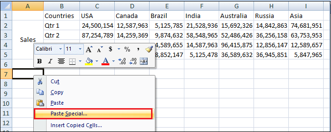
- Select the cell where you want to paste this data set, i.e. G10.
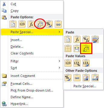
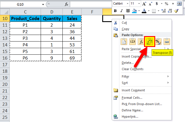
- When you enable right-click on the mouse, the paste option appears. You must then select the 4th option, i.e. Transpose (As mentioned in the below screenshot)
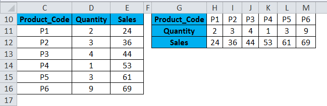
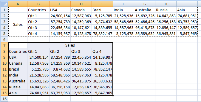
- On selecting the transpose option, your dataset gets copied in that cell range starting from cell G10 to M112.
- Apart from the above procedure, you can also use a shortcut key to convert columns to rows in excel.
- Copy the selected cells by pressing Ctrl + C.
- Select the cell where you need to copy this data set, i.e. G10.
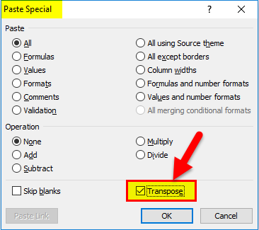
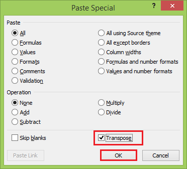
- Click on Alt + E + S, paste special dialog box popup window appears, in that select or click on the box of Transpose option, it will result or convert column data to rows data in excel.
Data that is copied is called source data, and when this source data is copied to other ranges, i.e. pasted data, which is referred to as transposed data.
Note: In the other direction where you are going to copy raw or source data, you have to ensure to select the same number of cells as the original set of cells so that there is no overlapping with the original dataset. In the above-mentioned example, there are 7-row cells that are arranged vertically. So when we copy this dataset to the horizontal direction, it should contain 7 column cells towards the other direction so that the overlapping does not occur with the original dataset.
Example #2
Sometimes, when you have huge number of columns, column data at the end is not visible, and it does not fit to screen. In this scenario, you can change its orientation from the current horizontal range to the vertical range with the help of the paste special option in excel.
- The table contains months and their serial number (From columns C to W).
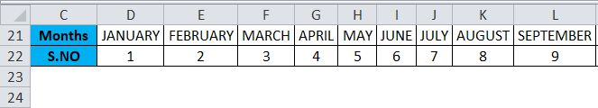
- Select the whole table range, i.e. all the cells with the dataset in a spreadsheet.
- Copy the selected cells by pressing Ctrl + C.
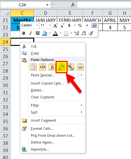
- Select the cell where you need to copy this data set, i.e. C24.
- When you right-click on the mouse, the paste options appear, in that you have to select 4th option, i.e. Transpose (Below mentioned screenshot)
- On selecting the transpose option, your dataset gets copied in that cell range starting from cell C24.
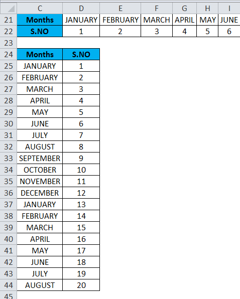
In the transposed data, all the data values are visible and clear as compared to the source data.
Disadvantages of using Paste special option:
- Sometimes copy-paste option creates duplicates.
- If you have used the Paste special option in excel to convert columns to rows, the transposed cells (or arrays) are not linked to each other with source data, and it does not get updated when you try to change data values in source data.
Example #3
Transpose function: It converts columns to rows and rows to columns in excel.
The syntax or formula for the Transpose function is:
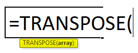
- Array: It is a range of cells that you need to convert or change their orientation.
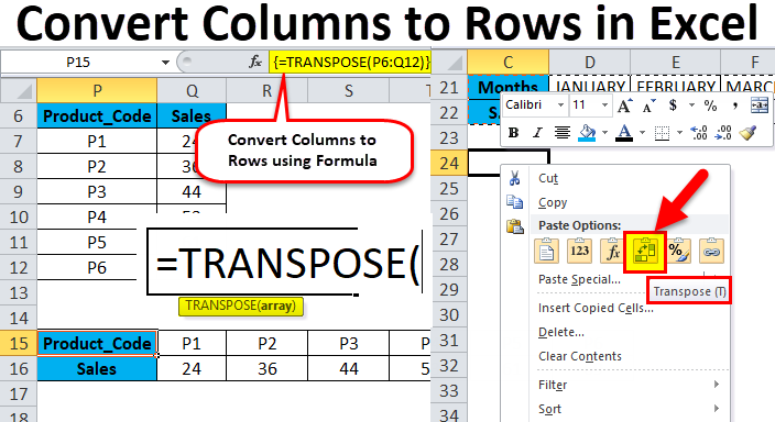
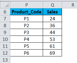
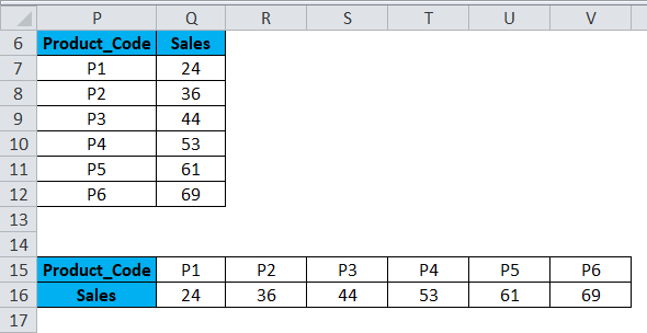
In the below example, the Pharma sales table contains medicine product code in column P (P7 to P12), and sales data in column Q (Q7 to Q12).
Check out the number of rows & columns in the source data which you want to transpose.
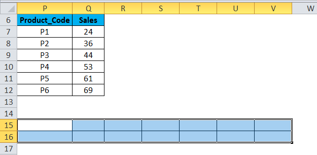
i.e. Initially, count the number of rows and columns in your original source data (7 rows & 2 columns) which is vertically positioned. Now select the same number of blank cells, but in the other direction (Horizontal), i.e. (2 rows & 7 columns)
- Prior to entering the formula, select the empty cells, i.e. from P15 to V16.
- With the empty cells selected, Type the transpose formula in cell P15. i.e. = TRANSPOSE (P6:Q12).
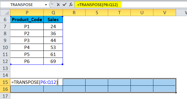
- Since the formula needs to be applied for the whole range, press Ctrl + Shift + Enter to make it an array formula.
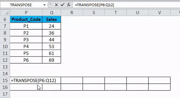
Now you can check the dataset; here, columns are converted to rows with datasets.
Advantages of the TRANSPOSE function:
- The main benefit or advantage of using the TRANSPOSE function is that transposed data or the rotated table retains the connection with the source table data, and whenever you change the source data, the transposed data also changes accordingly.
Things to Remember about Convert Columns to Rows in Excel
- Paste special option can also be used for other tasks, i.e. Add, Subtract, Multiply, and Divide between datasets.
- #VALUE error occurs while selecting the cells, i.e. If the number of columns and rows selected in transposed data are not equal to the rows and columns of the source data.
Recommended Articles
This has been a guide to Columns to Rows in Excel. Here we have discussed how to convert columns to rows in excel using transpose along with practical examples and a downloadable excel template. Transpose can help everyone to convert multiple Columns to Rows in excel easily and quickly. You can also go through our other suggested articles –
- COLUMNS Formula in Excel
- Add Rows in Excel Shortcut
- Column Header in Excel
- VBA Columns
Microsoft Excel is nothing but using data in columns and rows. When you are preparing data inExcel, sometime it is necessary to convert data in a column to a row and vice versa. This article explains step by step instructions on how to convert a column of an Excel sheet into a row. This is useful especially when you have data in table format and struggling to convert the columns of the table to rows along with the complete data. If you are frustrated with slow Excel, learn more on how to fix slow Excel and speed up data processing.
Example Data in a Table
Assume you have data in a table in an excel sheet as shown in the picture beside. Now you want to convert the complete table from columns to rows format. Copying and pasting each cell is a time consuming and error prone process.

Using Transpose Function
Microsoft Excel offers a simple functionality called “Transpose” to do such a difficult task in a few clicks. Follow the below steps to understand the transpose functions.
- Select the complete table data and copy to clipboard using Ctl+C shortcut.
- Right click on the cell where you want to paste it.
- Click on the option “Paste Special” from the context menu as shown in the picture below.
- A new popup window will open as shown below.
- Click on the checkbox “Transpose” and then click on “OK” button.

Now all your table data is transposed from rows to column format. This can be used for a single row or column to a big table of data spread into multiple columns and rows.
Directly Using Paste Special
When you right click on a cell, you also can click on the “Arrow” mark next to “Past Special” to see complete paste options including “Transpose” function as shown in the below picture.

Using Paste Options Control
Whenever you paste content in a cell you shall notice a small button appearing as “Paste Options (Ctrl)”. Once you used “Transpose” function, it will appear automatically in the paste options as a frequently used option. Hence from next time onwards, just copy the table and paste it in a cell where you want and click on the “Paste Options (Ctrl)” to use “Transpose” option.

Microsoft Excel for Mac
Similar to Windows version, you can use transpose function in Microsoft Excel for Mac also. After copying the content, simply right click on the cell where you want to paste and choose “Transpose” option. This will paste the content by converting rows into columns.

Alternatively, you can choose “Paste Special…” to open the dialog box. Here, you can check the “Transpose” option and click “OK” to paste the transposed data.

You can also press “Control + Command + V” keyboard shortcuts to open paste special dialog box.
There are two methods of doing this:
- Excel Ribbon Method
- Mouse Method
Let us take the below example to understand this process.
Table of contents
- How to Convert Columns to Rows in Excel?
- #1 Using Excel Ribbon – Convert Columns to Rows with copy and paste
- #2 Using Mouse – Converting Columns to Rows (Or Vise-Versa)
- Things to Remember
- Recommended Articles
You can download this Convert Columns to Rows Excel Template here – Convert Columns to Rows Excel Template
#1 Using Excel Ribbon – Convert Columns to Rows with copy and paste
We have the sales data location-wise.

This data is very useful for us, but we want to see this data in vertical order so that it will be easy to compare.
We must follow the below steps for converting columns to rows:
- We must select the whole data and go to the “HOME” tab.
- Then, we must click on the “Copy” option under the “Clipboard” section. You may refer to the below screenshot. Else, press “CTRL +C” keys to copy the data.

- Then, we must click on any blank cell where we want to see the data.
- Next, we must click on the “Paste” option under the “Clipboard” section. You may refer to the below screenshot.

- As a result, this will open a “Paste” dialog box. Then, choose the option “Transpose,” as shown below.

- Consequently, it will convert the columns to rows and display the data as we want.
The result is shown below:

Now, we can put the filter and see the data differently.
#2 Using Mouse – Converting Columns to Rows (Or Vise-Versa)
Let us take another example to understand this process.
We have some student score data subject-wise.

Now, we have to convert this data from columns to rows.
Follow the below steps for doing this:
- Step 1: We must first select the whole data and right-click. As a result, it will open a list of items. Now, we must click on the “Copy” option from the list. You may refer to the below screenshot.

- Step 2: We need to click on any blank cell where we want to paste this data.
- Step 3: Again, right-click and select Paste Special optionPaste special in Excel allows you to paste partial aspects of the data copied. There are several ways to paste special in Excel, including right-clicking on the target cell and selecting paste special, or using a shortcut such as CTRL+ALT+V or ALT+E+S.read more.

- Step 4: Again, it will open a “Paste Special” dialog box.
- Step 5: Then, click on the “Transpose option,” as shown in the below screenshot.
- Step 6: Lastly, we must click on the “OK” button.

Now our data is converted from columns to rows. The final result is shown below:

In other ways, when we move our cursor or mouse on “Paste Special” option, it will again open a list of options as shown below:

Things to Remember
- Converting columns to rows or vice-versa both methods also work when we want to convert a single column to a row or vice-versa.
- This option is very handy and saves a lot of time while working.
Recommended Articles
This article is a guide to Convert Columns to Rows in Excel. We discuss switching columns to rows in Excel using the ribbon and mouse method, practical examples, and a downloadable Excel template. You may learn more about Excel from the following articles: –
- Count Rows in Excel
- How to Convert Excel to CSV?
- Convert Text to Columns in Excel
- Row Limit in Excel
- MMULT in Excel
Reader Interactions
We all look at data differently. For example, some people create Microsoft Excel spreadsheets with the main fields horizontal. Others prefer data flipped vertically in columns. Sometimes these preferences lead to a scenario where you want to switch data. In this tutorial, I’ll show how to switch rows and columns using the Transpose feature.
The Layout Problem
I was recently given a large Microsoft Excel spreadsheet that contained vendor evaluation information. The information was useful, but I couldn’t use tools like Auto Filter because of the way the data was organized. I would also have issues if I needed to import the original source table into a database. A simple example is shown below.

Instead, I want to have the Company names displayed vertically in Column A and the Data Attributes displayed horizontally in Row 1. This would make it easier for me to do the analysis. For example, I can’t easily filter for California vendors with the original table.
What is Excel’s Transpose Function
In simple terms, the transpose feature changes your columns’ orientation (vertical range) and rows (horizontal range). My original data rows would become columns, and my columns would become rows. So this fixes my layout problem above without me having to retype my original data. And the system would adjust for column labels.
The transpose function is pretty versatile. For example, you can use the feature in Excel formulas or with paste options. However, there are some differences based on which method you use.
Convert Columns to Rows Using Paste Special
The steps outlined below were done using Microsoft Office 365, but recent Microsoft Excel versions will work.
- Open the spreadsheet you need to change. You may also download the example sheet at the end of this tutorial.
- Click the first cell in your cell range such as A1.
- Shift-click the last cell of the range. Your data set should highlight.
- From the Home tab, select Copy or type Ctrl + c.
- Select the new cell where you would like to copy your transposed data.
- Right-click in that cell and select the Transpose icon from the Paste Options.

✪ As you hover over the Paste options, you can see the data layout change.
You should now see Excel switched the columns and rows. You can resize your columns to suit your needs.
These two data sets are independent. You can delete cells from the top set and it will not impact the transposed set.

When using this method, your original formatting is maintained. For example, if I added a yellow background to my original cells B1:G1, the same background color would be applied. The same is true if I used red text on cell E:5.
Use Transpose Function in a Formula
As I mentioned, Excel has multiple ways for you to switch columns to rows or vice versa. This second way utilizes a formula and array. The result is the same except your original data, and the new transposed data are linked. As a result, you may lose some of your original formatting. For example, colored text and styles came across, but not cell fill colors.
- Open your Excel sheet.
- Click a blank cell where you want your converted data. I’m using A7.
- Type =transpose.
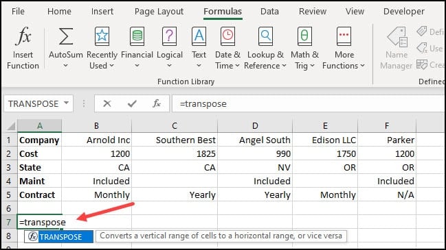
✪ Notice how Excel provides a tooltip showing for Transpose – “Converts a vertical range of cells to a horizontal range and vice versa“.
- Finish the formula by adding a ( and highlighting the cell range we wish to swap.
- Type ) to close the range.
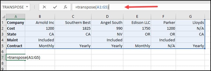
- Press Enter.
✪ If you’re not using Microsoft 365, you’ll probably need to press CTRL + SHIFT + Enter
Differences in Transpose Options
While these two methods produce similar results, there are differences. In the first paste method, whatever action I take on a cell is independent of the transposed version. I could delete the original values, and nothing would happen to the columns I swapped.
In contrast, the Transpose formula version is tethered to the original data. So, for example, if I change the value in B2 from 1200 to 1500, the new value will automatically update in B8. However, the reverse isn’t true. If I change any transposed cells, the original set will not change. Instead, I will get a #SPILL error, and my transposed data will disappear.

Transpose Formula & Blank Cells
Another difference with using the Transpose formula is it will convert blank cells to “0”s.

The fix for this quirk is to use an IF statement to the formula that keeps the blanks cells as blanks.
=TRANSPOSE(IF(A1:G5="","",A1:G5))Alternatively, you could do a search and replace on the zeros.
Now that we’ve shown you how to transpose data in Excel, try playing around with the practice worksheet below. You’ll be swapping your rows and columns in Excel in no time. And while you likely work with multiple rows, you can convert one Excel column to row.
Show Me How Video
Click the image below to see a short video showing how to switch columns and rows without a formula.
![]()
Tutorial Resources
Hand-picked Tutorials
- Beginner’s Guide to XLOOKUP
- How to Use Excel VLOOKUP
- How to Use Excel Auto Filter
- How to Extract Text from a Cell in Excel
- How to Highlight Cells in Excel with Conditional Formatting
#1 Using Excel Ribbon – Convert Columns to Rows with copy and paste
- Select the whole data and go to the HOME tab.
- Click on the Copy option under the Clipboard section.
- Then click on any blank cell where you want to see the data.
- Click on the Paste option under the Clipboard section.
- This will open a Paste dialogue box.
Contents
- 1 How do I make columns into rows in Excel?
- 2 How do I transpose one column into multiple rows?
- 3 How do you turn a column into a row in sheets?
- 4 How do I convert columns to rows in Excel on a Mac?
- 5 How do I swap columns in Excel?
- 6 How do I change columns to rows in Excel 2007?
- 7 How do you switch axis on Excel?
- 8 How do I transpose multiple columns to rows in Excel?
- 9 How do I convert data from one cell into multiple rows?
- 10 How do you transpose convert columns and rows into a single column?
- 11 How do I paste vertical data horizontally in sheets?
- 12 What does transpose mean in Excel?
- 13 How do I paste vertical data horizontally in Excel?
- 14 How do you switch rows in Excel?
- 15 How do I move columns and rows in Excel?
- 16 How do I change from horizontal to vertical in Excel 2007?
- 17 How do I paste vertical to horizontal in Excel 2007?
- 18 Why won’t Excel let me switch row column?
- 19 How do I convert multiple rows and columns to columns and rows in Excel?
- 20 Is there a way to do text to rows in Excel?
How to convert rows into columns in Excel – the basic solution
- Select and copy the needed range.
- Right click on a cell where you want to convert rows to columns.
- Select the Paste Transpose option to rotate rows to columns.
How do I transpose one column into multiple rows?
Transpose a single column to multiple columns with formulas
- In a blank cell C1, please enter this formula:=OFFSET($A$1,COLUMNS($A1:A1)-1+(ROWS($1:1)-1)*5,0), and then drag the fill handle from C1 to G1, see screenshot:
- Then go on dragging the fill handle down to the range as far as you need.
How do you turn a column into a row in sheets?
Here’s how you can use it to turn rows into columns in Google Spreadsheets.
- Double-click on the field where you want to start your new table.
- Type “=” and add “TRANSPOSE”.
- After that, Google Spreadsheets will show you how this function should be used and how it should look like.
How do I convert columns to rows in Excel on a Mac?
To change columns into rows quickly, follow these steps:
- Select a cell range and choose Edit→Copy.
- Select a destination cell.
- Choose Edit→Paste Special.
- Select the Transpose check box and then click OK.
How do I swap columns in Excel?
Press and hold the Shift key, and then drag the column to a new location. You will see a faint “I” bar along the entire length of the column and a box indicating where the new column will be moved. That’s it! Release the mouse button, then leave the Shift key and find the column moved to a new position.
How do I change columns to rows in Excel 2007?
Right-click in the white area of the chart and choose Select Data. In the Select Data Source box, choose Switch Row/Column, as the thumbnail shows below.
How do you switch axis on Excel?
How to switch axes in excel
- Click on the chart and choose the Design tab,
- Go to Data >> Switch Row / Column.
- Now, the X-axis switched with the Y-axis without the need for transposing data.
How do I transpose multiple columns to rows in Excel?
Select the new cell where you would like to copy your transposed data. Right-click in that cell and select the Transpose icon under Paste.
Convert Columns & Rows Using Paste & Transpose
- Open the spreadsheet you need to change.
- Click the first cell of your data range such as A1.
- Shift-click the last cell of the range.
How do I convert data from one cell into multiple rows?
Split cells
- Click in a cell, or select multiple cells that you want to split.
- Under Table Tools, on the Layout tab, in the Merge group, click Split Cells.
- Enter the number of columns or rows that you want to split the selected cells into.
How do you transpose convert columns and rows into a single column?
After free installing Kutools for Excel, please do as below:
- Select the cross table you want to convert to list, click Kutools > Range > Transpose Table Dimensions.
- In Transpose Table Dimension dialog, check Cross table to list option on Transpose type section, select a cell to place the new format table.
How do I paste vertical data horizontally in sheets?
To accomplish that maneuver, follow these steps:
- Select the vertical data.
- Type Ctrl C to copy.
- Click in the first cell of the horizontal range.
- Type Alt E, then type S to open the Paste Special dialog.
- Choose the Transpose checkbox as shown in Figure 1.
- Click OK.
What does transpose mean in Excel?
The TRANSPOSE function returns a vertical range of cells as a horizontal range, or vice versa.Use TRANSPOSE to shift the vertical and horizontal orientation of an array or range on a worksheet.
How do I paste vertical data horizontally in Excel?
Select the first cell of destination column, right click and select the Transpose (T) in the Paste Options section of the right-clicking menu. See below screenshot: And now the row is copied horizontally and pasted as one column vertically.
How do you switch rows in Excel?
Move Rows in Excel
- Select the row that you want to move.
- Hold the Shift Key from your keyboard.
- Move your cursor to the edge of the selection.
- Click on the edge (with left mouse button) while still holding the shift key.
- Move it to the row where you want this row to be shifted.
How do I move columns and rows in Excel?
Hold down OPTION and drag the rows or columns to another location. Hold down SHIFT and drag your row or column between existing rows or columns. Excel makes space for the new row or column.
How do I change from horizontal to vertical in Excel 2007?
How to Reconfigure a Horizontal Row to a Vertical Column in Excel
- Select all the rows or columns that you want to transpose.
- Click on a cell in an unused area of your worksheet.
- Click on the arrow below the “Paste” item and select “Transpose.” Excel pastes in your copied rows as columns or your copied columns as rows.
How do I paste vertical to horizontal in Excel 2007?
To change vertical data in a column to horizontal data in a row:
- Copy the vertical data.
- Find the cell you want to insert the data, and then click on it to select.
- Select the Paste button, but click on the down arrow – and a pop up menu of choices appears (these are your Paste Special options).
Why won’t Excel let me switch row column?
The way to fix this is to switch the rows and the columns. The problem is that the Switch Row/Column button on the Chart Tools Design tab is grayed out. Apparently, you have to edit and select the data to switch the rows and columns.Click the Select Data button.
How do I convert multiple rows and columns to columns and rows in Excel?
How to use the macro to convert row to column
- Open the target worksheet, press Alt + F8, select the TransposeColumnsRows macro, and click Run.
- Select the range that you want to transpose and click OK:
- Select the upper left cell of the destination range and click OK:
Is there a way to do text to rows in Excel?
Excel does not have the Text to Row tool like Text to Column. We will use the Transpose tool to convert our Text to Rows.
Содержание
- How to Transpose Excel Columns to Rows
- The Layout Problem
- What is Excel’s Transpose Function
- Convert Columns to Rows Using Paste Special
- Use Transpose Function in a Formula
- Differences in Transpose Options
- Transpose Formula & Blank Cells
- Show Me How Video
- Excel convert data from column to row
- Excel convert data from column to row
- VBA Code – convert data from column to row
- Convert all columns to a single column
- Convert all columns to a multiple columns
- Convert Columns to Rows in Excel
- How to Convert Columns to Rows in Excel?
- #1 Using Excel Ribbon – Convert Columns to Rows with copy and paste
- #2 Using Mouse – Converting Columns to Rows (Or Vise-Versa)
- Things to Remember
- Recommended Articles
How to Transpose Excel Columns to Rows
We all look at data differently. For example, some people create Microsoft Excel spreadsheets with the main fields horizontal. Others prefer data flipped vertically in columns. Sometimes these preferences lead to a scenario where you want to switch data. In this tutorial, I’ll show how to switch rows and columns using the Transpose feature.
The Layout Problem
I was recently given a large Microsoft Excel spreadsheet that contained vendor evaluation information. The information was useful, but I couldn’t use tools like Auto Filter because of the way the data was organized. I would also have issues if I needed to import the original source table into a database. A simple example is shown below.
Excel Spreadsheet Needing to Swap Columns & Rows
Instead, I want to have the Company names displayed vertically in Column A and the Data Attributes displayed horizontally in Row 1. This would make it easier for me to do the analysis. For example, I can’t easily filter for California vendors with the original table.
What is Excel’s Transpose Function
In simple terms, the transpose feature changes your columns’ orientation (vertical range) and rows (horizontal range). My original data rows would become columns, and my columns would become rows. So this fixes my layout problem above without me having to retype my original data. And the system would adjust for column labels.
The transpose function is pretty versatile. For example, you can use the feature in Excel formulas or with paste options. However, there are some differences based on which method you use.
Convert Columns to Rows Using Paste Special
The steps outlined below were done using Microsoft Office 365, but recent Microsoft Excel versions will work.
- Open the spreadsheet you need to change. You may also download the example sheet at the end of this tutorial.
- Click the first cell in your cell range such as A1.
- Shift-click the last cell of the range. Your data set should highlight.
- From the Home tab, select Copy or type Ctrl + c .
Copying the current Excel data
- Select the new cell where you would like to copy your transposed data.
- Right-click in that cell and select the Transpose icon from the Paste Options.
![]() Choose the Transpose option
Choose the Transpose option
✪ As you hover over the Paste options, you can see the data layout change.
You should now see Excel switched the columns and rows. You can resize your columns to suit your needs.
These two data sets are independent. You can delete cells from the top set and it will not impact the transposed set.
![]() Transposed data under original.
Transposed data under original.
When using this method, your original formatting is maintained. For example, if I added a yellow background to my original cells B1:G1, the same background color would be applied. The same is true if I used red text on cell E:5.
Use Transpose Function in a Formula
As I mentioned, Excel has multiple ways for you to switch columns to rows or vice versa. This second way utilizes a formula and array. The result is the same except your original data, and the new transposed data are linked. As a result, you may lose some of your original formatting. For example, colored text and styles came across, but not cell fill colors.
- Open your Excel sheet.
- Click a blank cell where you want your converted data. I’m using A7.
- Type =transpose.
![]() Typing transpose formula
Typing transpose formula
✪ Notice how Excel provides a tooltip showing for Transpose – “Converts a vertical range of cells to a horizontal range and vice versa“.
- Finish the formula by adding a ( and highlighting the cell range we wish to swap.
- Type ) to close the range.
![]() Transpose formula and range
Transpose formula and range
- Press Enter .
✪ If you’re not using Microsoft 365, you’ll probably need to press CTRL + SHIFT + Enter
Differences in Transpose Options
While these two methods produce similar results, there are differences. In the first paste method, whatever action I take on a cell is independent of the transposed version. I could delete the original values, and nothing would happen to the columns I swapped.
In contrast, the Transpose formula version is tethered to the original data. So, for example, if I change the value in B2 from 1200 to 1500, the new value will automatically update in B8. However, the reverse isn’t true. If I change any transposed cells, the original set will not change. Instead, I will get a #SPILL error, and my transposed data will disappear.
![]() Error when changing transposed cell
Error when changing transposed cell
Transpose Formula & Blank Cells
Another difference with using the Transpose formula is it will convert blank cells to “0”s.
![]() Transpose converted blanks to 0’s
Transpose converted blanks to 0’s
The fix for this quirk is to use an IF statement to the formula that keeps the blanks cells as blanks.
Alternatively, you could do a search and replace on the zeros.
Now that we’ve shown you how to transpose data in Excel, try playing around with the practice worksheet below. You’ll be swapping your rows and columns in Excel in no time. And while you likely work with multiple rows, you can convert one Excel column to row.
Show Me How Video
Click the image below to see a short video showing how to switch columns and rows without a formula.
Источник
Excel convert data from column to row
This Excel VBA tutorial explains how to convert data from column to row (transform one column data to one row).
You may also want to read:
Excel convert data from column to row
Different database have different structure. Some database put similar data in the same column with different rows, while some database put data in different columns. .Let’s take an example.
Type 1: all payment types are arranged in the same column
| Employee ID | Payment Type | Amount |
| 1 | Salary | 10000 |
| 1 | Allowance | 1000 |
| 2 | Salary | 10000 |
| 3 | Salary | 10000 |
| 4 | Salary | 10000 |
Type 2: each column for each payment type
| Employee ID | Salary | Allowance |
| 1 | 10000 | 1000 |
| 2 | 10000 | |
| 3 | 10000 | |
| 4 | 10000 |
In this tutorial, I will demonstrate how to use VBA to convert data from column to row (from type 2 to type 1).
VBA Code – convert data from column to row
Please note that when I wrote this Macro, I only tested the scenarios in my below examples. For any other exceptional scenarios that I am not aware, my Macro may not function probably (I don’t know what I don’t know).
Press ALT+F11 and then paste the below code in a new Module
Convert all columns to a single column
A little explanation for this code with an example. In the below Table, my goal is to move each salary and bonus column from column D to I to the same column (column D). For each newly added row, I want column A to C to repeat.
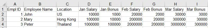
In the parameter line of code, I need to set the followings
Run the Macro and get the below result.
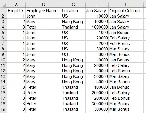
Column E is a new column created to indicate which column the data in column D originally came from. Column D header has to be manually change as it is the original header before conversion, so it is more appropriate to change it to “Amount”.
Convert all columns to a multiple columns
Suppose I want to convert all data columns to fit into column D (Salary) and column E (Bonus). Use the same Macro as above but update the below parameter to 2.
Run the Macro and get the below result.

Similar to the above example, column F is the new column to indicate where column D and E data originally came from. Column D and E headers should be renamed appropriately, such as “Salary” and “Bonus”.
Источник
Convert Columns to Rows in Excel


How to Convert Columns to Rows in Excel?
There are two methods of doing this:
- Excel Ribbon Method
- Mouse Method
Let us take the below example to understand this process.
Table of contents
#1 Using Excel Ribbon – Convert Columns to Rows with copy and paste
We have the sales data location-wise.
This data is very useful for us, but we want to see this data in vertical order so that it will be easy to compare.
We must follow the below steps for converting columns to rows:
- We must select the whole data and go to the “HOME” tab.
Then, we must click on the “Copy” option under the “Clipboard” section. You may refer to the below screenshot. Else, press “CTRL +C” keys to copy the data.
Then, we must click on any blank cell where we want to see the data.
Next, we must click on the “Paste” option under the “Clipboard” section. You may refer to the below screenshot.

As a result, this will open a “Paste” dialog box. Then, choose the option “Transpose,” as shown below.

Consequently, it will convert the columns to rows and display the data as we want.
The result is shown below:

Now, we can put the filter and see the data differently.
#2 Using Mouse – Converting Columns to Rows (Or Vise-Versa)
Let us take another example to understand this process.
We have some student score data subject-wise.
Now, we have to convert this data from columns to rows.
Follow the below steps for doing this:
- Step 1: We must first select the whole data and right-click. As a result, it will open a list of items. Now, we must click on the “Copy” option from the list. You may refer to the below screenshot.
- Step 2: We need to click on any blank cell where we want to paste this data.
- Step 3: Again, right-click and select Paste Special optionPaste Special OptionPaste special in Excel allows you to paste partial aspects of the data copied. There are several ways to paste special in Excel, including right-clicking on the target cell and selecting paste special, or using a shortcut such as CTRL+ALT+V or ALT+E+S.read more .
- Step 4: Again, it will open a “Paste Special” dialog box.
- Step 5: Then, click on the “Transpose option,” as shown in the below screenshot.
- Step 6: Lastly, we must click on the “OK” button.
Now our data is converted from columns to rows. The final result is shown below:
In other ways, when we move our cursor or mouse on “Paste Special” option, it will again open a list of options as shown below:
Things to Remember
- Converting columns to rows or vice-versa both methods also work when we want to convert a single column to a row or vice-versa.
- This option is very handy and saves a lot of time while working.
Recommended Articles
This article is a guide to Convert Columns to Rows in Excel. We discuss switching columns to rows in Excel using the ribbon and mouse method, practical examples, and a downloadable Excel template. You may learn more about Excel from the following articles: –
Источник
Home / Excel Formulas / How to Change Column to Row (Vice Versa) in Excel
In Excel, if you want to change columns to rows, you can use the TRANSPOSE function. With this function, all you need to do is select a range with equivalent cells from where you want to add the changed data, refer to the range, and use CONTROL + SHIFT + ENTER.
In the following example, you have a list of names and ages. And we need to change these two columns into rows.

Steps to Change Columns to Rows
- First, in the range D1:H2, enter the TRANSPOSE function.
- Next, refer to the range A1:B6.
- After that, type the closing parentheses.
- In the end, press and hold CRTL + SHIFT and press ENTER.

=TRANSPOSE(A1:B6)As you can see in the above example, we have successfully converted our columns into rows.
To understand how the transpose function works, you need to understand that it takes the array (range) you specify into it and then converts vertical cells into horizontal cells and vice versa.
But there is one thing that you need to take care of that you need to select the same number of cells oppositely. And you need to use CONTROL + SHIFT + ENTER to make this function work.
Here’s one more thing, once you create TRANSPOSE works in a dynamic way, once you change a value in any of the cells from the original cells, that value will also be changed in the transposed range.
And if you want to change the transposed range into values and don’t want to connect it with the original values, you can use paste a special value, or select the range using the keyboard shortcut Ctrl + C and then Alt + V ⇢ V.
As you know that people look at Excel data in their own way. Having data in rows might be sometimes needed to flip into columns or vice versa. Converting column data into rows and rows’ data into columns merely requires you to follow simple steps. For instance, if an Excel spreadsheet has data in horizontal cells, it might be possible that your boss prefers that data to be flipped vertically.
In this case, you will have to transpose Excel data to accommodate your preference. In Excel, you can use multiple methods for Excel flip rows and columns.
Before diving into the explanation of methods, let’s have a look at what is Transpose function used in Excel.
What is Transpose Function in Excel?
Using the transpose function let your data change its orientation such as the vertical range of your columns’ orientation and the horizontal range of your rows’ orientation. The transpose function is purely handy as well as versatile. For instance, this function could be used in Excel formulas or with paste options. Well, below you will find some differences that let you decide which method you should use.
Two major methods are described here for Excel flip rows and columns.
- Excel Ribbon Method
- Mouse Method
Let’s grab details with examples!
Excel Flip Rows and Columns with Copy and Paste
Below in this image, you can see the sales data location-wise.
This data is presented in horizontal order, whereas we need this data to be in the vertical orientation. Changed orientation will help us in comparison. Here are the easy to follow steps for converting columns to rows:
- Go to the Home tab after selecting the entire data.
- Under the Clipboard menu, choose the Copy option. Or else you may press CTRL + C for copying the data.

- Now, click on any blank cell from where you need the data to be.
- Hit the Paste option given under the Clipboard menu. See the image below.

A Paste dialogue box will open up. Now, select the option “Transpose.”

Doing this will flip the column to rows and make the orientation as we needed. Below is the final look of the converted datasheet.

Now, you can apply filters and see the data differently.
Excel Flip Rows and Columns with Mouse
Following these steps not only flip rows into columns, but you can even flip columns into rows as well. Let’s get into the final process.
Below in this image, you can see subject wise data of some students.

The above data is presented in columns and we will convert it into rows.
Here are the steps to follow:
- Select the entire data and right-click on it. You will see some options and choose Copy from the list.

- Now, click on an empty cell where you need to put that copied data.
- Once again, right-click and choose Paste Special option.

- A paste special dialogue box will appear once again. Choose the Transpose option and click on the OK button.

- Now, you can see the changed orientation of this data from columns to rows. Below you can see the final look in the image.

Moving your cursor on Paste Special option, you will see a list of options as you can see in the image below:

Flipping Multiple Rows and Columns in Excel Right from another Workbook
You have gone through two different methods to convert rows into columns or vice versa. The above method is perfect in case you need to flip rows into columns from another workbook with the help of an Excel desktop. To do this, you will have to keep both spreadsheets open for completing the copy and pasting work as explained earlier.
On the other hand, Excel Online does not work for different workbooks. Here you will not find the Paste Transpose option.

That’s why it is ideal to opt for the Transpose function for converting columns into rows and rows into columns.
Excel Flip Rows and Columns using VBA Macro
Using VBA can help you in executing multiple functions specifically when you need some customized functioning. If you are good at coding, VBA is for you. You can make all sorts of changes with just a few codes.
For instance, below you can see a coding script that lets you enjoy flipping rows into columns or vice versa:
Sub TransposeColumnsRows()
Dim SourceRange As Range
Dim DestRange As Range
Set SourceRange = Application.InputBox(Prompt:=”Please select the range to transpose”, Title:=”Transpose Rows to Columns”, Type:=8)
Set DestRange = Application.InputBox(Prompt:=”Select the upper left cell of the destination range”, Title:=”Transpose Rows to Columns”, Type:=8)
SourceRange.Copy
DestRange.Select
Selection.PasteSpecial Paste:=xlPasteAll, Operation:=xlNone, SkipBlanks:=False, Transpose:=True
Application.CutCopyMode = False
End Sub
Sub RowsToColumns()
Dim SourceRange As Range
Dim DestRange As Range
Set SourceRange = Application.InputBox(Prompt:=”Select the array to rotate”, Title:=”Convert Rows to Columns”, Type:=8)
Set DestRange = Application.InputBox(Prompt:=”Select the cell to insert the rotated columns”, Title:=”Convert Rows to Columns”, Type:=8)
SourceRange.Copy
DestRange.Select
Selection.PasteSpecial Paste:=xlPasteAll, Operation:=xlNone, SkipBlanks:=False, Transpose:=True
Application.CutCopyMode = False
End Sub
- Once this code is used, you have to go to the Visual Basic Editor (VBE). Use your mouse and go to the Developer tab => Visual Basic or else use the keyboard and press ALT + F11.

- Go to Insert => Module, in VBE.

- Copy and paste the script into the window.

- Shut down the VBE and go to Developer => Macros. You will find RowsToColumns macro.
- Click on the Run option.

- Choose the array to rotate and the cell to add the rotated columns.

All done!
Things to Consider When Converting Columns to Rows in Excel
You know one usage of Paste Special option mentioned above. In reality, you can use it for other purposes as well including Add, Multiply, Subtract, and Divide between datasets.
When you are selecting the cells, you may find #VALUE error, for instance, if the transposed data don’t have equal number of rows and columns to the number of rows and columns of the source data.
You store your information or data in various rows and columns. It can be a lot to keep track of. After incorrectly entering data, one of the most common mistakes is transposing columns and rows. Some people create Excel spreadsheets with the main fields horizontal. Others prefer the data vertically in columns. Sometimes these preferences lead to a scenario where you want to transpose Excel data.
With Excel, the option of copy/paste the entries into the other place or start over would be wrong because it can paste all entries into the same row or same column. There’s a really easy fix in the Paste Special menu that allows you to reverse your mistakes and columns to rows without starting over.
If you have a worksheet with data in columns that you need to rotate to rearrange it in rows, use the Transpose feature. With it, you can quickly switch data from columns to rows, or vice versa.
Transposing data in Excel is a task familiar to many users. You often build a complex table to realize that it makes perfect sense to rotate it for better analysis or presentation of data in graphs.
Microsoft must have anticipated this issue because they offer several methods to switch your columns and rows around. These solutions work in all versions of Excel 2016, 2013, 2010, 2007, and lower.
Convert Rows to Columns in Excel using Paste
Suppose you have a dataset similar to shown below. The country names are organized in columns, but the list of countries is too long, so we did better change columns to rows for the table to fit within the screen:
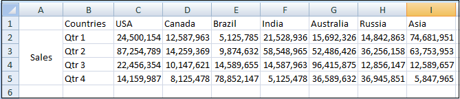
To switch rows to columns, you need to follow the following steps, such as:
Step 1: Select the original data of your table.
To quickly select the whole table, i.e., all the cells with data in a spreadsheet, press Ctrl + Home and then Ctrl + Shift + End.
Step 2: Copy the selected cells either by right-clicking the selection or choosing Copy from the context menu or by pressing Ctrl + C.
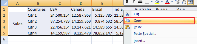
Step 3: Select the first cell of the destination range.
Be sure to select a cell that falls outside of the range containing your original data so that the copy areas and paste areas do not overlap.
For example, if you currently have 9 columns and 5 rows, the converted table will have 5 columns and 9 rows.
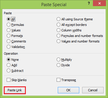
Step 4: Right-click the destination cell and choose Paste Special from the context menu.
Step 5: And then tick mark on the Transpose checkbox.
Step 6: Click on the OK button. You will get the transposed result of the table.
Note. If your source data contain formulas, properly use relative and absolute references depending on whether they should be adjusted or remained locked to certain cells.
As you have seen, the Paste Special feature lets you perform row to column or column to row transformations. This method also copies your original data format, which adds one more argument in its favor.
However, this approach has two drawbacks that prevent it from being called a perfect solution for transposing data in Excel:
- It is not well suited for rotating fully-functional Excel tables. If you copy the whole table and then open the Paste Specialdialog, you will find the Transpose option disabled. In this case, you need to copy the table without column headers or convert it to a range first.
- In Paste Special option, Transpose does not link the new table with the original data, so it is well suited only for one-time conversions. Whenever the source data change, you’d need to repeat the process and rotate the table.
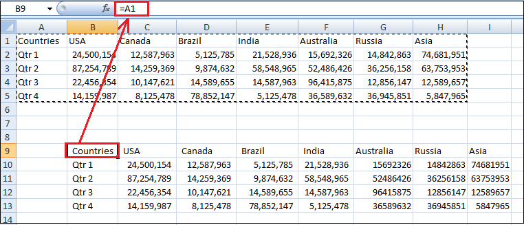
How to Transpose a Table and Link with Original Data
Let’s see how you can switch rows to columns using the familiar Paste Special technique but connect the resulting table to the original dataset.
The best thing about this approach is that whenever you change the source table’s data, the flipped table will reflect the changes and update accordingly. Follow these steps to transpose the table and link it with the original data.
Step 1: Copy the rows you want to convert to columns or columns to be changed to rows.
Step 2: Select an empty cell in the same or another sheet.
Step 3: Open the Paste Special dialog, as explained above, and click Paste Link in the lower left-hand corner.
You will get a result something like that:
Step 4: Select the new table and open Excel’s Find and Replace dialog or press Ctrl + H to get to the Replace tab straight away.
Step 5: Replace all «=» characters with «xxx» or any other characters that do not exist anywhere in your real data.
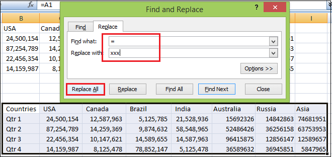
This will turn your table into something, as you see in the below screenshot. Now you need to follow these two more steps.
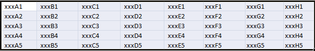
Step 6: Copy the table with «xxx» values, and then use Paste Special button and Transpose to flip columns to rows.
Step 7: Finally, open the Find and Replace dialog one more time to reverse the change, i.e., replace all «xxx» with «=» to restore the links to the original cells.
This way is a bit long but elegant solution. The only drawback of this approach is that the original formatting gets lost in the process, and you will need to restore it manually.
How to Convert Columns to Rows using Formulas
A simple way to dynamically convert columns to rows in Excel is by using the TRANSPOSE or INDEX/ADDRESS formula. These formulas also keep the connections to the original data but work differently.
1. Convert rows to columns using TRANSPOSE function
The TRANSPOSE function is specially designed for transposing data in Excel. This function has the following syntax.
In this example, we are going to convert the same table that lists countries by sales.
You need to follow the following steps to convert the table scenario by using the TRANSPOSE function.
Step 1: Count the number of rows and columns in your original table and select the same number of blank cells, but in the other direction or sheet.
Our sample table has 8 columns and 5 rows, including headings. Since the TRANSPOSE function will change columns to rows, we select a range of 5 columns and 8 rows.
Step 2: In the selected empty cells, write the below formula
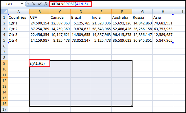
Step 3: Since our formula needs to be applied to multiple cells, press Ctrl + Shift + Enter to make it an array formula.
You will get the table in which columns are converted to rows and rows into columns, as shown below.
Advantages of TRANSPOSE Function
The main benefit of using the TRANSPOSE function is that the rotated table retains the source table’s connection. Whenever you change the source data, the transposed table will change accordingly.
Disadvantages of TRANSPOSE Function
- The original table formatting is not saved in the converted table.
- If there are any empty cells in the original table, the transposed cells will contain 0 instead. To fix this problem, use the combination of the TRANSPOSE function and the IF function.
- You cannot edit any cells in the rotated table because it is very much dependent on the source data. If you try to change some cell value, you will end up with the «You cannot change part of an array» error.
- This function is good and easy-to-use, but it certainly lacks flexibility and therefore may not be the best way to go in many situations.
2. Convert column to row using INDIRECT and ADDRESS functions
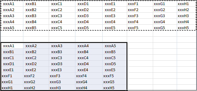
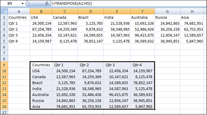
The below example will be using a combination of two functions. This is a little bit tricky. Suppose you have data in 5 columns and 5 rows, follow these steps to convert the table using the INDIRECT/ADDRESS function.
Step 1: Enter the below formula in the leftmost cell of the destination range and press the Enter key.
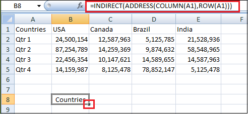
Step 2: Copy the formula rightward and downwards to as many rows and columns as needed by dragging the small black cross in the lower right-hand corner of the selected cells.
All of the columns are switched to rows in your newly created table, and rows are switched to columns.
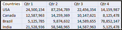
If your data starts in some row other than 1 and column other than A, you will have to use a bit more complex formula:
A1 is the top-left-most cell of your source table. Also, remember the use of absolute and relative cell references.
However, the transposed cells look very plain and dull in color compared to the original data. To restore the original formatting, just follow these three simple steps:
Step 1: Copy the original table.
Step 2: Select the resulting table.
Step 3: Right-click the resulting table, choose the Paste Options and then click on the Formatting button.
How this formula works
Now you know how to use the combination of the INDIRECT/ADDRESS function, you may want to understand what the formula is actually doing.
- As its name suggests, the INDIRECT function is used to reference a cell indirectly. But the real power of INDIRECT is that it can turn any string into a reference, including a string that you build up using other functions and other cells’ values. And this is exactly what we are going to do.
- We have used 3 more functions in the formula, such as ADDRESS, COLUMN, and ROW.
- The ADDRESS function obtains the cell address by the row and column numbers you specify, respectively.
- In our formula, we supply the coordinates in the reverse order, and this is what actually does the trick! In other words, this part of the formula ADDRESS(COLUMN(A1), ROW(A1)) swaps rows to columns, i.e., takes a column number and changes it to a row number, then takes a row number and turns it to a column number.
- Finally, the INDIRECT function outputs the rotated data.
Advantages of INDIRECT/ADDRESS Function
- This formula provides a more flexible way to turn rows into columns in Excel.
- It allows making any changes in the transposed table because you use a regular formula, not an array formula.
Disadvantages of INDIRECT/ADDRESS Function
The formatting of the ordinal data is lost. At the same time, you can quickly restore it.
Transpose Data VBA Macro in Excel
To automate the conversion of columns to rows in Excel, you can use the following macro:
NOTE: Transposing with VBA has a limitation of 65536 elements. In case your array exceeds this limit, the extra data will be silently discarded.
How to Convert Columns to row Using macro
With the macro inserted in your workbook, follow the below steps to rotate your table scenario.
Step 1: Open the target worksheet and press Alt + F8 key.
Step 2: Select the TransposeColumnsRows macro and click on the Run button.
Step 3: Select the range that you want to transpose and click on the OK button.
Step 4: Select the upper-left cell of the destination range.
Step 5: And click on the OK button.