

This Excel tutorial explains how to change column headings from numbers (1, 2, 3, 4) back to letters (A, B, C, D) in Excel 2016 (with screenshots and step-by-step instructions).
Question: In Microsoft Excel 2016, my Excel spreadsheet has numbers for both rows and columns. How do I change the column headings back to letters such as A, B, C, D?
Answer: Traditionally, column headings are represented by letters such as A, B, C, D. If your spreadsheet shows the columns as numbers, you can change the headings back to letters with a few easy steps.
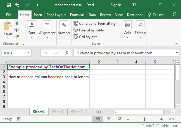
In the example below, the column headings are numbered 1, 2, 3, 4 instead of the traditional A, B, C, D values that you normally see in Excel. When the column headings are numeric values, R1C1 reference style is being displayed in the spreadsheet.
To change the column headings to letters, select the File tab in the toolbar at the top of the screen and then click on Options at the bottom of the menu.

When the Excel Options window appears, click on the Formulas option on the left. Then uncheck the option called «R1C1 reference style» and click on the OK button.

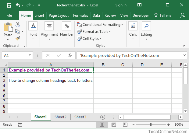
Now when you return to your spreadsheet, the column headings should be letters (A, B, C, D) instead of numbers (1, 2, 3, 4).
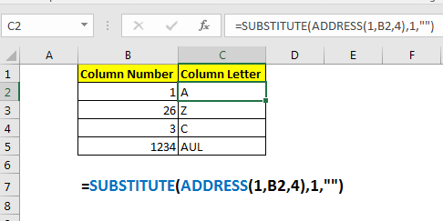
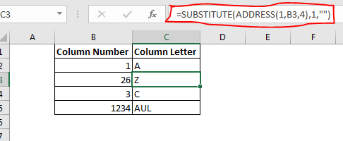
In this example, the goal is to convert an ordinary number into a column reference expressed in letters. For example, the number 1 should return «A», the number 2 should return «B», the number 26 should return «Z», etc. The challenge is that Excel can handle over 16,000 columns, so the number of letter combinations is large. One way to solve this problem is to construct a valid address with the number and extract just the column from the address. This is the approach explained below. For reference, the formula in C5 is:
=SUBSTITUTE(ADDRESS(1,B5,4),"1","")
ADDRESS function
Working from the inside out, the first step is to construct an address that contains the correct column reference. We can do this with the ADDRESS function, which will return the address for a cell based on a given row and column number. For example:
=ADDRESS(1,1) // returns "$A$1"
=ADDRESS(1,2) // returns "$B$1"
=ADDRESS(1,26) // returns "$Z$1"
By providing 4 for the optional abs_num argument, we can get a relative reference:
=ADDRESS(1,1,4) // returns "A1"
=ADDRESS(1,2,4) // returns "B1"
=ADDRESS(1,26,4) // returns "Z1"
Note the result from ADDRESS is always a text string. We don’t particularly care about the row number, we only care about the column number, so we use 1 for row_num in all cases. In the worksheet shown, we get the column number from column B and use 1 for row number like this:
ADDRESS(1,B5,4)
As the formula is copied down, ADDRESS creates a valid address using each number in column B. The maximum number of columns in an Excel worksheet is 16,384, so the final column in a worksheet is «XFD».
SUBSTITUTE function
Now that we have an address with the column reference we want, we simply need to remove the row number. One way to do this is with the SUBSTITUTE function. For example, assuming we have an address like «A1», we can use SUBSTITUTE like this:
=SUBSTITUTE("A1","1","") // returns "A"
We are telling SUBSTITUTE to look for «1» and replace it with an empty string («»). We can confidently do this in all cases, because we’ve hardcoded the row number as 1 inside the ADDRESS function. The final formula in C5 is:
=SUBSTITUTE(ADDRESS(1,B5,4),"1","")
In brief, ADDRESS cerates the cell reference and returns the result to SUBSTITUTE, which removes the «1».
TEXTBEFORE function
A cleaner way to extract the column reference from the address is to use the TEXTBEFORE function like this:
=TEXTBEFORE(ADDRESS(1,B5,4),"1")
Here, we treat «1» as a delimiter and ask TEXTBEFORE for all text before the delimiter. The result from this formula is the same as above.
Microsoft Excel has patterns such as A, B, C, AA, BB, CC, AD, AA, AAB, and AAZ. Column 1 is named as A, B as 2, and 27 as AA. Therefore, finding a column letter is easy and possible, given its corresponding column number is easy. To convert a column number to the letter in Excel, you can follow the following steps. It is important to note that this function only converts integers into their corresponding alphanumeric text character. The column or row headings on the physical worksheet are not changed in appearance.
Steps to convert a column Number
It is important to note that we deal with 26 characters from A-Z. Remember, we don’t have zero among these characters since A represents 1 while Z represents 26. There are two ways to tackle this problem;
- Say you have the number 676, it is still possible to get its base representation.
- Divide and get a remainder of 26
-
To get rid of zero, we get (25 26)to base 26; thus, its symbolic representation is YZ
It is also important to know how to convert the column headings into letters in Excel
1. Go to File Tab

2. Select Options
3. The Excel Options window appears. Click on the Formulas option

4. Ensure the R1CA option reference style is unchecked

5. Press on OK
6. The column numbers will turn into letters

How to turn column letters into numbers
Sometimes you might need to convert column letters to numbers. You can achieve it in the following easy steps.
1. Click on the File tab

2. Navigate down and click on options

3. Click on Formulas on the popup window that popups.

4. Navigate to the working with formulas section and check the box on the R1C1 reference style

5. Click ok
6. The column labels will turn to numbers

How to convert column numbers to text using VBA
1. Press Alt +F11
2. Copy and paste the code below
Sub ColNumToLetter()
Dim ColNumber As Long
Dim ColLetter As String
‘Input Column Number
ColNumber = 200
‘Convert To Column Letter
ColLetter = Split(Cells(1, ColNumber).Address, «$»)(1)
‘Display Result
MsgBox «Column » & ColNumber & » = Column » & ColLetter
End Sub
Save and run the macro
Some times we get the need of converting given column number into the column letter (A, B, C,..), since the excel addressing function works with column letters.
So there’s no function that converts the excel column number to column letter directly. But we can combine SUBSTITUTE function with ADDRESS function to get the column letter using column index.
Generic Formula
Column_number: the column number of which you want to get column letter.
Example: Covert excel number to column letter
Here we have some column numbers in B2:B5. We want to get corresponding column letter (A, B, C, etc) from that given number (1, 2, 3, etc.).
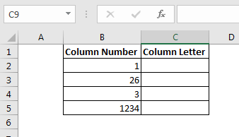
Apply above generic formula here to get column letter from column number.
Copy down this formula. You have the column letters in C2:C5.
How it works?
Well, this is a quite simple formula. The aim is to get first cell address of given column number. Then remove the row number to have only the column letter. We get the address of first cell of given column number using ADDRESS function.
ADDRESS(1,B2,4): Here B2 contains 1. This make translates to ADDRESS(1,1,4). The address FUNCTION returns the address at coordinate 1st row, 1st Column in relative format (4). This give us A1.
Now SUBSTITUTE function has SUBSTITUTE(A1,1,””). It replaces 1 with nothing (“”) from A1. This gives us A.
So yeah guys this how you can convert number to letter of column in excel. In our next tutorial, we will learn how to convert column letter to number. Till than, if you have any doubts regarding this article or any other topic in advanced excel, let us know in the comments section below.
Popular Articles:
The VLOOKUP Function in Excel
COUNTIF in Excel 2016
How to Use SUMIF Function in Excel
Содержание
- How to convert Excel column numbers into alphabetical characters
- Introduction
- More Information
- How to convert column number to letter
- Convert column number to letter using excel formula
- Convert column number to letter with VBA user defind function
- Convert column number to letter
- Related functions
- Summary
- Generic formula
- Explanation
- ADDRESS function
- SUBSTITUTE function
- TEXTBEFORE function
- How to convert column number to letter in Excel
- How to convert column number into alphabet (single-letter columns)
- How to convert Excel column number to letter (any column)
- Get column letter from column number using custom function Custom function
- How to get column letter of certain cell
- How to get column letter of the current cell
- How to create dynamic range reference from column number
How to convert Excel column numbers into alphabetical characters
Introduction
This article discusses how to use the Microsoft Visual Basic for Applications (VBA) function in Microsoft Excel to convert column numbers into their corresponding alphabetical character designator for the same column.
For example, the column number 30 is converted into the equivalent alphabetical characters «AD».
More Information
Microsoft provides programming examples for illustration only, without warranty either expressed or implied. This includes, but is not limited to, the implied warranties of merchantability or fitness for a particular purpose. This article assumes that you are familiar with the programming language that is being demonstrated and with the tools that are used to create and to debug procedures. Microsoft support engineers can help explain the functionality of a particular procedure, but they will not modify these examples to provide added functionality or construct procedures to meet your specific requirements.
The ConvertToLetter function works by using the following algorithm:
- Let iCol be the column number. Stop if iCol is less than 1.
- Calculate the quotient and remainder on division of (iCol — 1) by 26, and store in variables a and b .
- Convert the integer value of b into the corresponding alphabetical character (0 => A, 25 => Z) and tack it on at the front of the result string.
- Set iCol to the divisor a and loop.
For example: The column number is 30.
(Loop 1, step 1) The column number is at least 1, proceed.
(Loop 1, step 2) The column number less one is divided by 26:
29 / 26 = 1 remainder 3. a = 1, b = 3
(Loop 1, step 3) Tack on the (b+1) letter of the alphabet:
3 + 1 = 4, fourth letter is «D». Result = «D»
(Loop 1, step 4) Go back to step 1 with iCol = a
(Loop 2, step 1) The column number is at least 1, proceed.
(Loop 2, step 2) The column number less one is divided by 26:
0 / 26 = 0 remainder 0. a = 0, b = 0
(Loop 2, step 3) Tack on the b+1 letter of the alphabet:
0 + 1 = 1, first letter is «A» Result = «AD»
(Loop 2, step 4) Go back to step 1 with iCol = a
(Loop 3, step 1) The column number is less than 1, stop.
The following VBA function is just one way to convert column number values into their equivalent alphabetical characters:
Note This function only converts integers that are passed to it into their equivalent alphanumeric text character. It does not change the appearance of the column or the row headings on the physical worksheet.
Источник
How to convert column number to letter
This post explains that how to convert a column number to a column letter using formula in excel. How to convert column number to a column letter using user defined function in VBA.
Convert column number to letter using excel formula
if you want to convert column number to letter, you can use the ADDRESS function to get the absolute reference of one excel cell that contains that column number, such as, you can get the address of Cell B1, then you can use the SUBSTITUTE function to replace row number with empty string, so that you can get the column letter. So you can write down the following formula using the SUBSTITUTE function and the ADDRESS function.
Let’s see how this formula works:
The ADDRESS function returns an absolute reference for a cell at a given row and column number. And this formula returns A1. The returned address goes into the SUBSTITUTE function as its Text argument.
This formula will replace the old_text “1” with empty string for a string of cell reference returned by the ADDRESS. So it returns a letter.
Convert column number to letter with VBA user defind function
You can also create a new user defined function to convert column number to a column letter in Excel VBA:
1# click on “Visual Basic” command under DEVELOPER Tab.
2# then the “Visual Basic Editor” window will appear.
3# click “Insert” ->”Module” to create a new module named
4# paste the below VBA code into the code window. Then clicking “Save” button.
5# back to the current worksheet, then enter the below formula in Cell C1:
Источник
Convert column number to letter

Summary
To convert a column number to an Excel column letter (e.g. A, B, C, etc.) you can use a formula based on the ADDRESS and SUBSTITUTE functions. In the example shown, the formula in C5, copied down, is:
The result is the column reference as one or more letters.
Generic formula
Explanation
In this example, the goal is to convert an ordinary number into a column reference expressed in letters. For example, the number 1 should return «A», the number 2 should return «B», the number 26 should return «Z», etc. The challenge is that Excel can handle over 16,000 columns, so the number of letter combinations is large. One way to solve this problem is to construct a valid address with the number and extract just the column from the address. This is the approach explained below. For reference, the formula in C5 is:
ADDRESS function
Working from the inside out, the first step is to construct an address that contains the correct column reference. We can do this with the ADDRESS function, which will return the address for a cell based on a given row and column number. For example:
By providing 4 for the optional abs_num argument, we can get a relative reference:
Note the result from ADDRESS is always a text string. We don’t particularly care about the row number, we only care about the column number, so we use 1 for row_num in all cases. In the worksheet shown, we get the column number from column B and use 1 for row number like this:
As the formula is copied down, ADDRESS creates a valid address using each number in column B. The maximum number of columns in an Excel worksheet is 16,384, so the final column in a worksheet is «XFD».
SUBSTITUTE function
Now that we have an address with the column reference we want, we simply need to remove the row number. One way to do this is with the SUBSTITUTE function. For example, assuming we have an address like «A1», we can use SUBSTITUTE like this:
We are telling SUBSTITUTE to look for «1» and replace it with an empty string («»). We can confidently do this in all cases, because we’ve hardcoded the row number as 1 inside the ADDRESS function. The final formula in C5 is:
In brief, ADDRESS cerates the cell reference and returns the result to SUBSTITUTE, which removes the «1».
TEXTBEFORE function
A cleaner way to extract the column reference from the address is to use the TEXTBEFORE function like this:
Here, we treat «1» as a delimiter and ask TEXTBEFORE for all text before the delimiter. The result from this formula is the same as above.
Источник
How to convert column number to letter in Excel
 by Svetlana Cheusheva, updated on March 9, 2023
In this tutorial, we’ll look at how to change Excel column numbers to the corresponding alphabetical characters.
When building complex formulas in Excel, you may sometimes need to get a column letter of a specific cell or from a given number. This can be done in two ways: by using inbuilt functions or a custom one.
How to convert column number into alphabet (single-letter columns)
In case the column name consists of a single letter, from A to Z, you can get it by using this simple formula:
For example, to convert number 10 to a column letter, the formula is:
It’s also possible to input a number in some cell and refer to that cell in your formula:
=CHAR(64 + A2) 
How this formula works:
The CHAR function returns a character based on the character code in the ASCII set. The ASCII values of the uppercase letters of the English alphabet are 65 (A) to 90 (Z). So, to get the character code of uppercase A, you add 1 to 64; to get the character code of uppercase B, you add 2 to 64, and so on.
How to convert Excel column number to letter (any column)
If you are looking for a versatile formula that works for any column in Excel (1 letter, 2 letter and 3 letter), then you’ll need to use a bit more complex syntax:
With the column letter in A2, the formula takes this form:
=SUBSTITUTE(ADDRESS(1, A2, 4), «1», «») 
How this formula works:
First, you construct a cell address with the column number of interest. For this, supply the following arguments to the ADDRESS function:
- 1 for row_num (the row number does not really matter, so you can use any).
- A2 (the cell containing the column number) for column_num.
- 4 for abs_num argument to return a relative reference.
With the above parameters, the ADDRESS function returns the text string «A1» as the result.
As we only need a column letter, we strip the row number with the help of the SUBSTITUTE function, which searches for «1» (or whatever row number you hardcoded inside the ADDRESS function) in the text «A1» and replaces it with an empty string («»).
Get column letter from column number using custom function Custom function
If you need to convert column numbers into alphabetical characters on a regular basis, then a custom user-defined function (UDF) can save your time immensely.
The code of the function is pretty plain and straightforward:
Here, we use the Cells property to refer to a cell in row 1 and the specified column number and the Address property to return a string containing an absolute reference to that cell (such as $A$1). Then, the Split function breaks the returned string into individual elements using the $ sign as the separator, and we return element (1), which is the column letter.
Paste the code in the VBA editor, and your new ColumnLetter function is ready for use. For the detailed guidance, please see: How to insert VBA code in Excel.
From the end-user viewpoint, the function’s syntax is as simple as this:
Where col_num is the column number that you want to convert into a letter.
Your real formula can look as follows:
And it will return exactly the same results as native Excel functions discussed in the previous example: 
How to get column letter of certain cell
To identify a column letter of a specific cell, use the COLUMN function to retrieve the column number, and serve that number to the ADDRESS function. The complete formula will take this shape:
As an example, let’s find a column letter of cell C5:
=SUBSTITUTE(ADDRESS(1, COLUMN(C5), 4), «1», «»)
Obviously, the result is «C» 🙂 
How to get column letter of the current cell
To work out the letter of the current cell, the formula is almost the same as in the above example. The only difference is that the COLUMN() function is used with an empty argument to refer to the cell where the formula is:
=SUBSTITUTE(ADDRESS(1, COLUMN(), 4), «1», «») 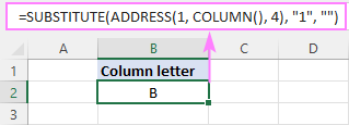
How to create dynamic range reference from column number
Hopefully, the previous examples have given you some new subjects for thought, but you may be wondering about the practical applications.
In this example, we’ll show you how to use the «column number to letter» formula for solving real-life tasks. In particular, we’ll create a dynamic XLOOKUP formula that will pull values from a specific column based on its number.
From the sample table below, suppose you wish to get a profit figure for a given project (H2) and week (H3). 
To accomplish the task, you need to provide XLOOKUP with the range from which to return values. As we only have the week number, which corresponds to the column number, we are going to convert that number to a column letter first, and then construct the range reference.
For convenience, let’s break down the whole process into 3 easy to follow steps.
- Convert a column number to a letter
With the column number in H3, use the already familiar formula to change it to an alphabetical character:
=SUBSTITUTE(ADDRESS(1, H3, 4), «1», «») 
Tip. If the number in your dataset does not match the column number, be sure to make the required correction. For example, if we had the week 1 data in column B, the week 2 data in column C, and so on, then we’d use H3+1 to get the correct column number.
To build a range reference in the form of a string, you concatenate the column letter returned by the above formula with the first and last row numbers. In our case, the data cells are in rows 3 through 8, so we are using this formula:
=SUBSTITUTE(ADDRESS(1, H3, 4), «1», «») & «3:» & SUBSTITUTE(ADDRESS(1, H3, 4), «1», «») & «8»
Given that H3 contains «3», which is converted to «C», our formula undergoes the following transformation:
And produces the string C3:C8. 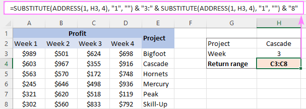
Make a dynamic range reference
To transform a text string into a valid reference that Excel can understand, nest the above formula in the INDIRECT function, and then pass it to the 3 rd argument of XLOOKUP:
=XLOOKUP(H2, E3:E8, INDIRECT(H4), «Not found») 
To get rid of an extra cell containing the return range string, you can place the SUBSTITUTE ADDRESS formula within the INDIRECT function itself:
=XLOOKUP(H2, E3:E8, INDIRECT(SUBSTITUTE(ADDRESS(1, H3, 4), «1», «») & «3:» & SUBSTITUTE(ADDRESS(1, H3, 4), «1», «») & «8»), «Not found») 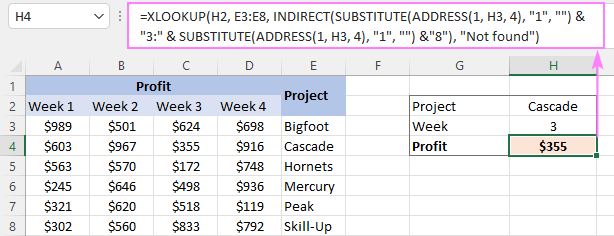
With our custom ColumnLetter function, you can get a more compact and elegant solution:
=XLOOKUP(H2, E3:E8, INDIRECT(ColumnLetter(H3) & «3:» & ColumnLetter(H3) & «8»), «Not found»)
That’s how to find a column letter from a number in Excel. I thank you for reading and look forward to seeing you on our blog next week!
Источник
This Excel tutorial explains how to use Excel Address Function and how to convert column number to column letter.
Excel Address Function is used to combine column number and row number to return Cell address in Text format.
Excel Address Function is most useful is converting column number to column letter, or use with Indirect Function to convert the Text address to Range Object.
Syntax of Excel Address Function
ADDRESS( row, column, [abs_num], [a1], [sheet_text] )
| row | Row number in number format | ||||||||||
| column | Column number in number format | ||||||||||
| [abs_num] | Optional, the style of Cell address
|
||||||||||
| [a1] | Optional, style of Referencing
|
||||||||||
| [sheet_text] | Add sheet name in the prefix of Cell address. You can type whatever you want, not necessary the worksheet name, it only puts this text in the address prefix. |
Example of Excel Address Function
| Formula | Value | Explanation |
| =ADDRESS(1,1) | $A$1 | Row 1 Column 1 = A1 |
| =ADDRESS(1,1,4) | A1 | Return A1 without absolute $ |
| =ADDRESS(1,1,4,0) | R[1]C[1] | Return R1C1 style of A1 |
| =ADDRESS(1,1,4,,”Sheet1″) | Sheet1!A1 | Add sheet name in address prefix |
Use Excel Address Function to convert column number to column letter
One important use of Address Function is to convert column number to column header.
For example, you have a column number 4, you want to convert to letter D.
| Formula | Value | Explanation | |
| Step 1 | =ADDRESS(1,4,4) | D1 | Put a dummy row number 1 in address, return relative reference |
| Step 2 | =SUBSTITUTE(ADDRESS(1,4,4),1,””) | D | Replace 1 as nothing |
After you have got the column letter, you can use it in another formula.
The below example shows how to get the D5 value using Indirect Function, which turns Text “D5” into actual Range value.
=INDIRECT(SUBSTITUTE(ADDRESS(1,4,4),1,"")&"5")
Recently I have answered a question in Microsoft Community that uses this skill, click here to read more.
If you want to know how it can be done in VBA, click here to read my other article.
Use Excel Column Function to convert column letter to column number
You can use Column Function to convert column letter to column number, which converts a Range to a column number. Since the Function argument is a Range, use indirect Function to convert the column letter to an actual Range. Similar to Address Function, put dummy row number 1 in the formula.
| Formula | Result |
| =COLUMN(INDIRECT(“A”&1)) | 1 |
| =COLUMN(INDIRECT(“Z”&1)) | 26 |
Convert column numbers to letters
In this example, we want to input the column number in the first column of the table then allow the second column to show the corresponding Excel column letter. Letter A corresponds to the first column in an Excel worksheet, B to the second column, C to the third column, and so on.
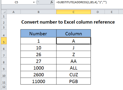
Figure 1. Convert column numbers to letters
To convert a column number to an Excel column letter (i.e, A, B, C, etc.) we will make use a formula that utilizes the ADDRESS and SUBSTITUTE functions.
The general formula would be
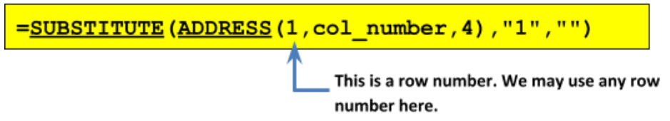
Figure 2. Convert column numbers to letters
In our example, the formula in cell C5 will be

Figure 3. Convert column numbers to letters
Using the ADDRESS Function
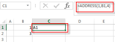
The ADDRESS function returns a text representation of a cell address. It is a built-in function in Excel that can be used as a look-up function. For example, the formula =ADDRESS(1,1) will return the value $A$1. The ADDRESS function can be entered as part of a formula or as a parameter within another function.
The first step is to generate an address that carries the column number. We will do this with the ADDRESS function, by providing 1 for row number (we can use any row number and this will be hard-coded, or fixed, in the formula), a column number from cell B5, and we will use 4 for the abs_num argument to get a relative reference to the cell address. Note that the four possible values for the abs_num argument are: 1 (or omitted) for absolute reference; 2 for absolute row and relative column reference; 3 for relative row and absolute column reference; and 4 for relative reference.
With the information provided, our ADDRESS function will return the text string “A1”. We will then use the SUBSTITUTE function to remove the number portion of the text and retain only the column letter.
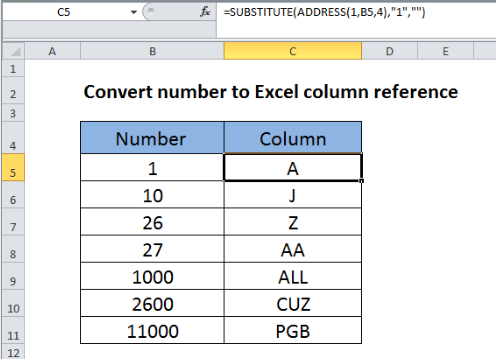
Figure 4. Convert column numbers to letters
Using the SUBSTITUTE Function
The SUBSTITUTE function is used to replace specific parts of a text with another by means of matching. For example, the formula =SUBSTITUTE(“123-456-789”, “-”, “”) will return “123456789” because we specify in the formula to replace every occurrence of “-” in the main text with the null string (“”), thereby removing the dashes. Note that the SUBSTITUTE function is case-sensitive.
As mentioned, we will use the SUBSTITUTE function to remove the number portion of the text cell address reference and retain only the column letter. Here is how it’s done: In all cases, we can confidently locate “1” and then replace it with the null string (“”)
i.e., =SUBSTITUTE (“A1”,”1”,””).
This is because the number on the row is hard-coded as “1” inside the ADDRESS function.
Instant Connection to an Expert through our Excelchat Service
Most of the time, the problem you will need to solve will be more complex than a simple application of a formula or function. If you want to save hours of research and frustration, try our live Excelchat service! Our Excel Experts are available 24/7 to answer any Excel question you may have. We guarantee a connection within 30 seconds and a customized solution within 20 minutes.
This post explains that how to convert a column number to a column letter using formula in excel. How to convert column number to a column letter using user defined function in VBA.
Table of Contents
- Convert column number to letter using excel formula
- Convert column number to letter with VBA user defind function
- Related Formulas
- Related Functions
Convert column number to letter using excel formula
if you want to convert column number to letter, you can use the ADDRESS function to get the absolute reference of one excel cell that contains that column number, such as, you can get the address of Cell B1, then you can use the SUBSTITUTE function to replace row number with empty string, so that you can get the column letter. So you can write down the following formula using the SUBSTITUTE function and the ADDRESS function.
=SUBSTITUTE(ADDRESS(1,B1,4),"1"," ")
Let’s see how this formula works:
=ADDRESS(1,B1,4)
The ADDRESS function returns an absolute reference for a cell at a given row and column number. And this formula returns A1. The returned address goes into the SUBSTITUTE function as its Text argument.
=SUBSTITUTE(ADDRESS(1,B1,4),”1″,” “)
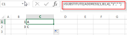
This formula will replace the old_text “1” with empty string for a string of cell reference returned by the ADDRESS. So it returns a letter.
Convert column number to letter with VBA user defind function
You can also create a new user defined function to convert column number to a column letter in Excel VBA:
1# click on “Visual Basic” command under DEVELOPER Tab.

2# then the “Visual Basic Editor” window will appear.
3# click “Insert” ->”Module” to create a new module named

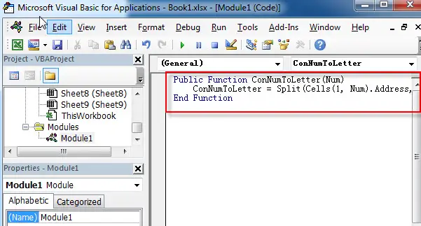
4# paste the below VBA code into the code window. Then clicking “Save” button.
Public Function ConNumToLetter(Collet)
    ConNumToLetter = Split(Cells(1, Collet).Address, "$")(1)
End Function
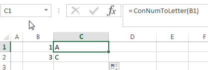
5# back to the current worksheet, then enter the below formula in Cell C1:
= ConNumToLetter(B1)
- Extract text after first comma or space
If you want to get substring after the first comma character from a text string in Cell B1, then you can create a formula based on the MID function and FIND function or SEARCH function …. - Convert column letter to number
If you want to convert a column letter to number, you can use a combination of the COLUMN function and the INDIRECT function to create an excel formula…..
- Excel ADDRESS function
The Excel ADDRESS function returns a reference as a text string to a single cell.The syntax of the ADDRESS function is as below:=ADDRESS (row_num, column_num, [abs_num], [a1], [sheet_text])…. - Excel Substitute function
The Excel SUBSTITUTE function replaces a new text string for an old text string in a text string.The syntax of the SUBSTITUTE function is as below:= SUBSTITUTE (text, old_text, new_text,[instance_num])….