
Column Header in Excel (Table of Contents)
- Introduction to Column Header in Excel
- How to Use Column Header in Excel?
Introduction to Column Header in Excel
Column Header is a very important part of excel as we work on different types of Tables in excel every day. Column Headers basically tell us the category of the data in that column to which it belongs. For example, if column A contains Date, then Column header for Column A will be “Date”, or suppose column B contains Names of the student, then column header for Column B will be “Student Name”. Column Headers are important in a way when a new person looks at your excel; he can understand the meaning of the data in those columns. It is also important because you need to remember how the data has been organized in your excel. So from the data organization standpoint, Column Headers play a very important role.
In this article, we will look at the best possible ways of how we can organize or format the column headers in excel. There are many ways of creating headers in excel. The three best possible ways of creating headers are below.
- Freezing Row/Column.
- Printing a header row.
- Creating a header in Table.
We will look at each way of creating a header one by one with the help of examples.
Suppose you are working on the data which has a large number of rows, and when you scroll down in the worksheet to look at some data, you may not be able to look at the Column Header. This is where Freeze Panes helps in excel. You can scroll down in the excel sheet without losing visibility to the column headers.
How to Use Column Header in Excel?
Column Header in Excel is very simple and easy. Let’s understand how to use the column Header in Excel with some examples.
You can download this Column Header Excel Template here – Column Header Excel Template
Example #1 – Freezing Row/Column
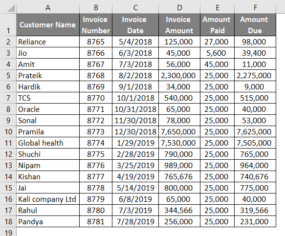
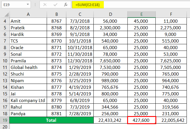
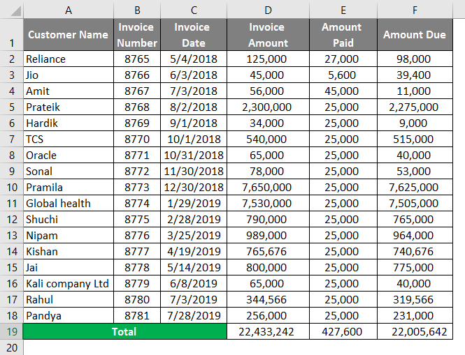
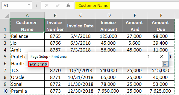
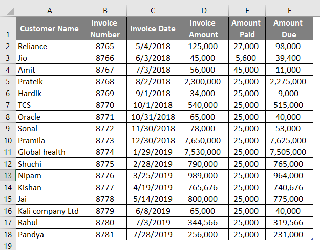
- Suppose there is data related to customers in excel, as shown in the below screenshot.
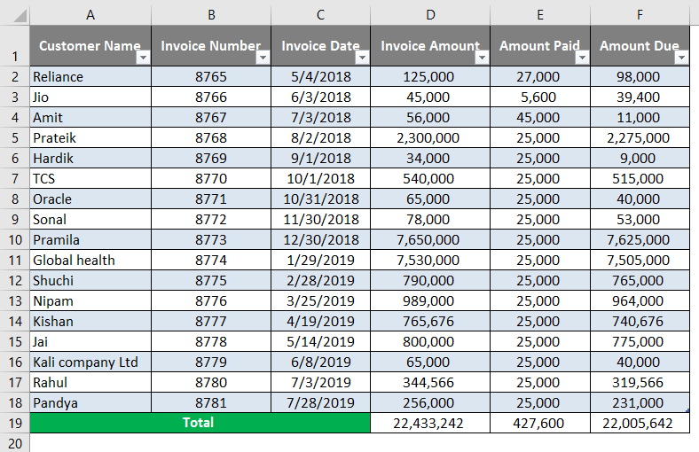
- Use SUM formula in cell D19.
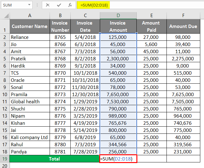
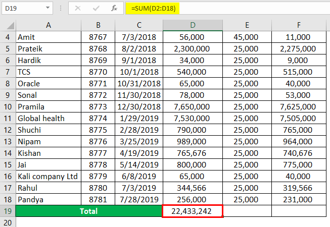
- After using the SUM formula, the output is shown below.
- The same formula is used in cell E19 and cell F19.
You need to follow the below steps to freeze the top row.
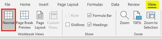
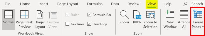
- Go to the View tab in Excel.
- Click on the Freeze Pane Option
- You will see three options after clicking on the Freeze Pane option. You need to select the “Freeze Top Row” option.
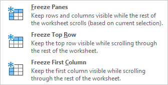
- Once you click on the “Freeze Top Row”, the top row will be freezer, and you scroll down in excel without losing visibility to excel. You can see in the below screenshot that Row 1, which has column headers, are still visible even when you scroll down.
Example #2 – Printing a Header Row
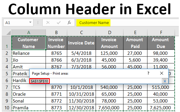
When you are working on large spreadsheets where data is spread across multiple pages and when you need to take a print out, it doesn’t fit well on one page. The printing job becomes frustrating as you are not able to see the column headers in print after the first page. In that scenario, there is a functionality in excel known as “Print Titles”, which helps set a row or rows to print at the top of every page. We will take a similar example which we have taken in Example 1.
Follow the below steps to use this functionality in Excel.
- Go to the Page Layout tab in Excel.
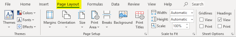
- Click on Print Titles.
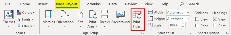
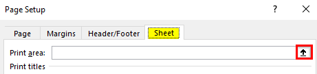
- After clicking on the Print Titles option, you will see the below window open for Page Set up in excel.
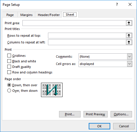
- In the Page Set up window, you will find different options that you can choose.
(a) Print Area
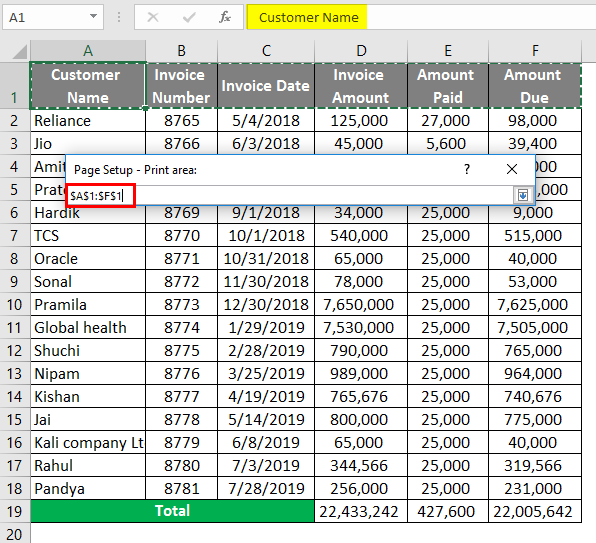
- To select Print Area, click on the button on the right side, as shown in the screenshot.
- After clicking on the button, the navigation window will open. You can select from Row 1 to Row 10 to print the first 10 rows.
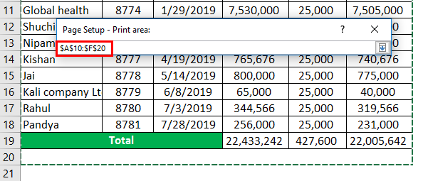
- If you want to print Row 11 to Row 20, you can select the Print Area as Row 11 to Row 20.
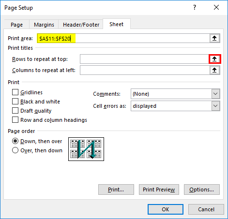
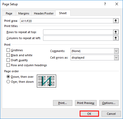
- Under Print Titles, you can find two options.
(b) Rows to Repeat at Top
This is where we need to select the column header, which we want to repeat on every page of the printout. To select Rows to repeat at the top, click on the button on the right side, as shown in the screenshot.
After clicking on the button, the navigation window will open. You can select Row 1, as shown in the below screenshot.
(C) Columns to Repeat at Left
This is the column that you want to see on the left, which will repeat on every page. We will keep it as blank as we don’t have any row headers in our table.
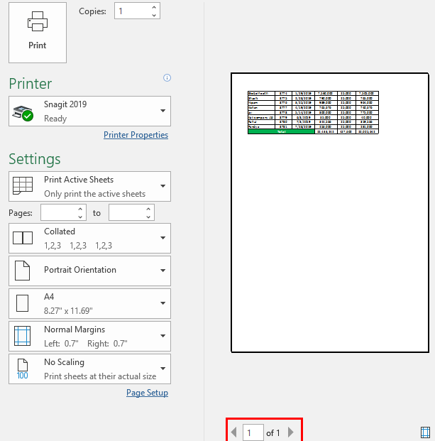
- Now click on the “Print Preview” option on the page setup as shown in the below screenshot to see the Print Preview. As you can see in the below screenshot, the print area is from Row 11 to Row 20, with the column headers in Row 1.
- Click on Ok in the Page setup window after exiting from Print Preview.
Example #3 – Creating a Header in a Table
One of the features in Excel is that you can convert your data into a Table. It automatically creates Headers when you convert your data into a table. But please take a note here that these headers are different from the Worksheet column heading or printed headers which we have seen earlier.
- We will take a similar example which we have taken earlier.
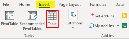
- Click on the “Insert” tab and then click on the “Table” button.
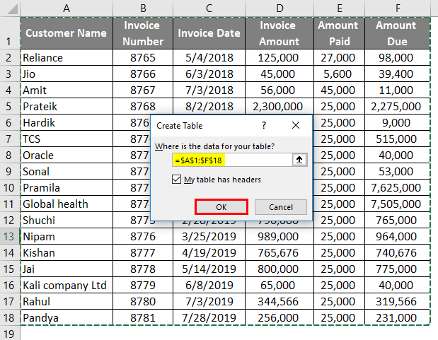
- After clicking on the “Table” option, you can give the range of data that you want to convert into the table and also select the checkbox of “My Table has Headers”, as shown in the below screenshot. The first row of your selection will automatically be assigned as column headers.
- Click Ok. You will see your data is converted into a Table.
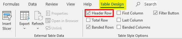
- You can Enable or Disable the Header row by going into the “Design” tab of the Table.
Things to Remember About Column Headers in Excel
- Always remember to format column headers differently and use Freeze panes to have visibility on the column header at all times. It will help you save time of scrolling up and down to understand data.
- Make sure to use the Print Area option and Rows to repeat at every page option while printing. This will make your printing job easy.
- Selection of Range and Column header is important while creating Table in Excel.
Recommended Article
This is a guide to Column Header in Excel. Here we discuss How to use Column Header in Excel along with practical examples and downloadable excel template. You can also go through our other suggested articles –
- Compare Two Columns in Excel for Matches
- Freeze Columns in Excel
- COLUMNS Formula in Excel
- Excel Header Row
Use a screen reader to create column headers in a table in Excel
Excel for Microsoft 365 Excel 2021 Excel 2019 Excel 2016 More…Less
This article is for people with visual or cognitive impairments who use a screen reader program such as Microsoft’s Narrator, JAWS, or NVDA with Microsoft 365 products. This article is part of the Microsoft 365 screen reader support content set where you can find more accessibility information on our apps. For general help, visit Microsoft Support home.
Use Excel with your keyboard and a screen reader to create descriptive column headers in an existing table. We have tested it with Narrator, JAWS, and NVDA, but it might work with other screen readers as long as they follow common accessibility standards and techniques.
Table headers also help people who use screen readers understand what the column is all about. In a long table, table headers replace the worksheet column headings so that they stay visible when you move through the table data. Table headers should not be confused with worksheet column headings or the headers for printed pages.
Notes:
-
New Microsoft 365 features are released gradually to Microsoft 365 subscribers, so your app might not have these features yet. To learn how you can get new features faster, join the Office Insider program.
-
To learn more about screen readers, go to How screen readers work with Microsoft 365.
Add column headers to an existing table
You can add column headers to a table even if you created your table without headers. You can also change the default header names directly in the worksheet.
For instructions on how to add column headers when creating a table, refer to Use a screen reader to insert a table in an Excel worksheet.
-
Place focus anywhere in the table.
-
Press Alt+J, T, and then O to add column headers.
-
To edit the default column header name, press the arrow keys until you hear with Narrator the column cell you want to edit, followed by «Editable, column,» and the default header name. With JAWS, you hear the default header name and the cell, followed by «Column header.» With NVDA, you hear the default header name and the cell.
-
Type the new header name.
See also
Use a screen reader to insert a table in an Excel worksheet
Use a screen reader to title a table in Excel
Keyboard shortcuts in Excel
Basic tasks using a screen reader with Excel
Set up your device to work with accessibility in Microsoft 365
Use a screen reader to explore and navigate Excel
Technical support for customers with disabilities
Microsoft wants to provide the best possible experience for all our customers. If you have a disability or questions related to accessibility, please contact the Microsoft Disability Answer Desk for technical assistance. The Disability Answer Desk support team is trained in using many popular assistive technologies and can offer assistance in English, Spanish, French, and American Sign Language. Please go to the Microsoft Disability Answer Desk site to find out the contact details for your region.
If you are a government, commercial, or enterprise user, please contact the enterprise Disability Answer Desk.
Need more help?
Want more options?
Explore subscription benefits, browse training courses, learn how to secure your device, and more.
Communities help you ask and answer questions, give feedback, and hear from experts with rich knowledge.
Find solutions to common problems or get help from a support agent.
Open the Spreadsheet
- Open the Spreadsheet.
- Open the Excel spreadsheet where you want to define your column headings.
- Use the Page Layout Tab.
- Click the “Page Layout” tab at the top of the ribbon, then find the Sheet Options area of the ribbon, which includes two small checkboxes under the Headings category.
Contents
- 1 How do you create column names in Excel?
- 2 What is column headings in Excel?
- 3 How do I make the first row in Excel a header?
- 4 How do I make column letters in Excel?
- 5 How do I insert column headings in Word?
- 6 How do I show column and row headings in Excel?
- 7 Where is the header row in Excel?
- 8 How do I keep column headers when scrolling in Excel?
- 9 How do I get the column name in Excel?
- 10 How do I convert row numbers to letters in Excel?
- 11 How do I get column names from column numbers in Excel?
- 12 How do I repeat headings in Excel?
- 13 What are the column headers in the table?
- 14 How can you create the first row of the table as the header of the table?
- 15 How do I change column headings in Excel 2010?
- 16 How do you see headings as you scroll around a report?
- 17 How do you keep row and column labels in view when scrolling?
- 18 How do I rename a column header in Excel?
- 19 Can’t see column headers in Excel?
- 20 How do you use flash fill in Excel?
How do you create column names in Excel?
Single Sheet
- Click the letter of the column you want to rename to highlight the entire column.
- Click the “Name” box, located to the left of the formula bar, and press “Delete” to remove the current name.
- Enter a new name for the column and press “Enter.”
In Excel and Google Sheets, the column heading or column header is the gray-colored row containing the letters (A, B, C, etc.) used to identify each column in the worksheet.used to identify each row in the worksheet.
With a cell in your table selected, click on the “Format as Table” option in the HOME menu. When the “Format As Table” dialog comes up, select the “My table has headers” checkbox and click the OK button. Select the first row; which should be your header row.
How do I make column letters in Excel?
To convert a column number to an Excel column letter (e.g. A, B, C, etc.) you can use a formula based on the ADDRESS and SUBSTITUTE functions. With this information, ADDRESS returns the text “A1”.
How do I insert column headings in Word?
To add column headings to a table in Word:
- Place your cursor in the first cell of the top row of the table.
- Type the name for the first column, and press Tab to move to the next column.
- Repeat step 2 for the remaining columns.
How do I show column and row headings in Excel?
On the Ribbon, click the Page Layout tab. In the Sheet Options group, under Headings, select the Print check box. , and then under Print, select the Row and column headings check box .
Row header or Row heading is the gray-colored column located on the left side of column 1 in the worksheet, which contains the numbers (1, 2, 3, etc.) where it helps out to identify each row in the worksheet.
How do I keep column headers when scrolling in Excel?
How to keep column header viewing when scrolling in Excel?
- Enable the worksheet you need to keep column header viewing, and click View > Freeze Panes > Freeze Top Row.
- If you want to unfreeze the column headers, just click View > Freeze Panes > Unfreeze Panes.
How do I get the column name in Excel?
Slightly manual but less VBA and a simpler formula:
- In a row of Excel, e.g. cell A1, enter the column number =column()
- In the row below, enter =Address(1,A1)
- This will provide the result $A$1.
How do I convert row numbers to letters in Excel?
To change the column headings to letters, select the File tab in the toolbar at the top of the screen and then click on Options at the bottom of the menu. When the Excel Options window appears, click on the Formulas option on the left. Then uncheck the option called “R1C1 reference style” and click on the OK button.
How do I get column names from column numbers in Excel?
- Try getColName = Cells(1, colNumber).Value. – Fadi.
- Columns in excel do not have names.
- @Scott Craner, you misunderstand me.
- Here is the answer to my question.
- getColName = Cells(1, colNumber).EntireColumn.Name.Name.
How do I repeat headings in Excel?
How to Repeat Excel Spreadsheet Column Headings at Top of Page
- Click the [Page Layout] tab > In the “Page Setup” group, click [Print Titles].
- Under the [Sheet] tab, in the “Rows to repeat at top” field, click the spreadsheet icon.
- Click and select the row you wish to appear at the top of every page.
What are the column headers in the table?
A table header is a row at the top of a table used to label each column. For example, in the below table there are three columns with a “Name,” “Date of Birth,” and “Phone” header.
In the table, right-click in the row that you want to repeat, and then click Table Properties. In the Table Properties dialog box, on the Row tab, select the Repeat as header row at the top of each page check box.
How do I change column headings in Excel 2010?
To change the column headings to letters, select the File tab in the toolbar at the top of the screen and then click on Options at the bottom of the menu. When the Excel Options window appears, click on the Formulas option on the left. Then uncheck the option called “R1C1 reference style” and click on the OK button.
How do you see headings as you scroll around a report?
Freeze Top Row
You want to be able to scroll through the data and always see the headings. You can use the Freeze Panes command on the View tab, in the Window group and then click on Freeze Top Row. A solid horizontal line will be drawn after rows 1.
How do you keep row and column labels in view when scrolling?
Select the cell below the rows and to the right of the columns you want to keep visible when you scroll. Select View > Freeze Panes > Freeze Panes.
How do I rename a column header in Excel?
Instead, rename them using Excel’s formula bar.
- Click “View” in Excel’s ribbon.
- Check the box marked “Formula Bar” in the Show group.
- Click the cell of the column header that you want to rename.
- Double-click the column’s name in the formula bar to select it.
- Type a new name.
Can’t see column headers in Excel?
Show or hide the Header Row
- Click anywhere in the table.
- Go to the Table tab on the Ribbon.
- In the Table Style Options group, select the Header Row check box to hide or display the table headers.
How do you use flash fill in Excel?
If Flash Fill doesn’t generate the preview, it might not be turned on. You can go to Data > Flash Fill to run it manually, or press Ctrl+E. To turn Flash Fill on, go to Tools > Options > Advanced > Editing Options > check the Automatically Flash Fill box.
For many small business owners, Microsoft Excel is not only a powerful tool for internal tracking and bookkeeping, but it can also be used to prepare documents for distribution to partners or customers. When creating a spreadsheet for distribution, controlling the spreadsheet’s appearance ensures it appears professional to colleagues and outside contacts. Excel offers two types of column headings; the letters the Excel assigns to each column, which you can toggle in both view and print modes, or the headings that you create yourself and place in the spreadsheet’s first row, which you can then freeze in place.
Understanding Excel Column Headers
Excel refers to rows by number and columns by letter, starting the first row at one and the first column with «A». For some purposes, this is fine, but you often want to add your own column labels in Excel specifying for yourself and other people using the spreadsheet what each column contains.
For instance, if each row is an employee record, you might label columns with headers such as «first name», «last name», «email address» and the like.
Default Excel Column Headings
-
Open the Spreadsheet
-
Open the Excel spreadsheet where you want to define your column headings.
-
Use the Page Layout Tab
-
Click the «Page Layout» tab at the top of the ribbon, then find the Sheet Options area of the ribbon, which includes two small checkboxes under the Headings category.
-
Check to Show Headings
-
Add or remove a check mark next to «View» to reveal or hide, respectively, the Excel headings on the spreadsheet. The headings for the columns and rows are linked, so you can only either see them both, or hide them both. The column headings will be letters and the row headings will be numbers.
-
Choose Whether to Print Headings
-
Place a check mark in the box next to «Print» to have Excel include the column and row headings on anything that you print out. These headings will appear on every page that you print, not just the first.
Customized Column Headings in Excel
-
Open the Spreadsheet
-
Open the spreadsheet where you want to have Excel make the top row a header row.
-
Add a Header Row
-
Enter the column headings for your data across the top row of the spreadsheet, if necessary. If your data is already present in the top row, right-click on the number «1» on the top of the left side of the spreadsheet and choose «Insert» from the pop-up menu to create a new top row, then enter your headings by typing in the appropriate cell.
-
Select the First Data Row
-
Click on the number «2» on the left side of the spreadsheet to select the second row, which is the now the first row under the headings and the first containing actual data.
-
Freeze the Headers in Place
-
Click the «View» tab in the ribbon menu, and then click the «Freeze Panes» button in the Window area of the ribbon. Your column headers now stay visible as you scroll down the spreadsheet, letting you see which column is which as you edit the document.
-
Configuring Printing Options
-
Click the «Page Layout» tab if you want your headers to print on every page of the spreadsheet. Click the arrow next to «Sheet Options» in the ribbon to open a small window. Check the box next to «Rows to repeat at top,» which shrinks the window and takes you back to the spreadsheet. Click the number one on the left side of the spreadsheet, and then click the small box again to return the window to its normal size. Click «OK» to save your changes.
Содержание
- What Is A Column Heading In Excel?
- What do you mean by column heading?
- What are row and column headings in Excel?
- How do I get column headings in Excel?
- What is a row heading in Excel?
- What is cell heading?
- What are headings and titles in a spreadsheet called?
- How do I get column headings on each page in Excel?
- How do you designate the first row as column headings?
- What is the difference between a page header and a heading on your worksheet?
- What is the row heading?
- What is row heading called?
- What is the row and column?
- How do you do a heading?
- How do you add a logo to a header in Excel?
- What is row with example?
- What are column headings in excel?
- What are headers in Excel?
- Where are headings in Excel?
- Excel Tutorial #08: How to create a column title
- What is AutoFilter in Excel?
- Where is the center header section in Excel?
- What is a sheet name code in Excel?
- Why can’t I see my header in Excel?
- How do I create a header row in Excel?
- What do you call the first column in a table?
- What is row and column headings in Excel?
- How do I make the first column a header in Excel?
- How To Create Column Headings In Excel?
- How do you create column names in Excel?
- What is column headings in Excel?
- How do I make the first row in Excel a header?
- How do I make column letters in Excel?
- How do I insert column headings in Word?
- How do I show column and row headings in Excel?
- Where is the header row in Excel?
- How do I keep column headers when scrolling in Excel?
- How do I get the column name in Excel?
- How do I convert row numbers to letters in Excel?
- How do I get column names from column numbers in Excel?
- How do I repeat headings in Excel?
- What are the column headers in the table?
- How can you create the first row of the table as the header of the table?
- How do I change column headings in Excel 2010?
- How do you see headings as you scroll around a report?
- How do you keep row and column labels in view when scrolling?
- How do I rename a column header in Excel?
- Can’t see column headers in Excel?
- How do you use flash fill in Excel?
What Is A Column Heading In Excel?
In Excel and Google Sheets, the column heading or column header is the gray-colored row containing the letters (A, B, C, etc.) used to identify each column in the worksheet. The column header is located above row 1 in the worksheet.used to identify each row in the worksheet.
What do you mean by column heading?
The column heading is a heading that identifies a column of a worksheet. Column headings are at the top of each column and are labeled A, B,… Z, AA, AB… . This example shows two columns, column A and column B.
What are row and column headings in Excel?
By default, Excel uses the A1 reference style, which refers to columns as letters (A through IV, for a total of 256 columns), and refers to rows as numbers (1 through 65,536). These letters and numbers are called row and column headings. To refer to a cell, type the column letter followed by the row number.
How do I get column headings in Excel?
Show or hide the Header Row
- Click anywhere in the table.
- Go to Table Tools > Design on the Ribbon.
- In the Table Style Options group, select the Header Row check box to hide or display the table headers.
What is a row heading in Excel?
A row heading identifies a row on a worksheet. Row headings are at the left of each row and are indicated by numbers.
What is cell heading?
Header cells are those that contain the information that is critical to understanding the raw data in a table. For example the number 210 is meaningless on its own, but becomes information if you know that it is the data for a) the number of properties in b) a given street.
What are headings and titles in a spreadsheet called?
Your Excel 2013 spreadsheets can benefit from page headers and fixed column titles, also called description rows.
How do I get column headings on each page in Excel?
How to Repeat Excel Spreadsheet Column Headings at Top of Page
- Click the [Page Layout] tab > In the “Page Setup” group, click [Print Titles].
- Under the [Sheet] tab, in the “Rows to repeat at top” field, click the spreadsheet icon.
- Click and select the row you wish to appear at the top of every page.
How do you designate the first row as column headings?
Enabling Customized Column Headers
With a cell in your table selected, click on the “Format as Table” option in the HOME menu. When the “Format As Table” dialog comes up, select the “My table has headers” checkbox and click the OK button. Select the first row; which should be your header row.
A page header automatically appears on every single printed page. Excel needs to be setup manually to repeat column headings.Page headers allow us to add important meta information in addition to the contents of a worksheet.
What is the row heading?
The row heading or row header is the gray-colored column located to the left of column 1 in the worksheet containing the numbers (1, 2, 3, etc.) used to identify each row in the worksheet.
What is row heading called?
The rows headings of a table are known as caption.
What is the row and column?
Rows are a group of cells arranged horizontally to provide uniformity. Columns are a group of cells aligned vertically, and they run from top to bottom.
How do you do a heading?
Add a heading
- Select the text you want to use as a heading.
- On the Home tab, move the pointer over different headings in the Styles gallery. Notice as you pause over each style, your text will change so you can see how it will look in your document. Click the heading style you want to use.
Go to Insert > Header or Footer > Blank. Double-click Type here in the header or footer area. Select Picture from File, choose your picture, and select Insert to add the picture.
What is row with example?
A row is a series of data banks laid out horizontally in a table or spreadsheet. For example, in the picture below, the row headers (row numbers) are numbered 1, 2, 3, 4, 5, etc. Row 16 is highlighted in red and cell D8 (on row  is the selected cell.
Источник
What are column headings in excel?
Last Update: Jan 03, 2023
This is a question our experts keep getting from time to time. Now, we have got the complete detailed explanation and answer for everyone, who is interested!
A header in excel: It is a section of the worksheet that appears at the top of each of the pages in the excel sheet or document. This remains constant across all the pages. It can contain information such as Page No., Date, Title or Chapter Name, etc.
Where are headings in Excel?
On the Insert tab, in the Text group, click Header & Footer. Excel displays the worksheet in Page Layout view. To add or edit a header or footer, click the left, center, or right header or footer text box at the top or the bottom of the worksheet page (under Header, or above Footer). Type the new header or footer text.
Excel Tutorial #08: How to create a column title
38 related questions found
What is AutoFilter in Excel?
Excel’s AutoFilter feature makes filtering out unwanted data in a data list as easy as clicking the AutoFilter button on the column on which you want to filter the data and then choosing the appropriate filtering criteria from that column’s drop-down menu.
Click the Insert tab, and click Header & Footer. This displays the worksheet in Page Layout view. The Header & Footer Tools Design tab appears, and by default, the cursor is in the center section of the header.
What is a sheet name code in Excel?
In Excel. . Using the sheet name code Excel formula requires combining the MID, CELL, and FIND functions into one formula. For example, if you are printing out a financial model. Discover the top 10 types onto paper or as a PDF, then you may want to display the sheet name on the top of each page.
The Advanced options of the Excel Options dialog box. Make sure the Show Row and Column Headers check box is selected. If cleared, then the header area is not displayed.
Go to the «Insert» tab on the Excel toolbar, and then click the “Header & Footer” button in the Text group to start the process of adding a header. Excel changes the document view to a Page Layout view. Click on the top of your document where it says “Click to Add Header,” and then type the header for your document.
What do you call the first column in a table?
The first column often presents information dimension description by which the rest of the table is navigated. This column is called «stub column». Tables may contain three or multiple dimensions and can be classified by the number of dimensions.
What is row and column headings in Excel?
In Excel and Google Sheets, the column heading or column header is the gray-colored row containing the letters (A, B, C, etc.) used to identify each column in the worksheet. . The row heading or row header is the gray-colored column located to the left of column 1 in the worksheet containing the numbers (1, 2, 3, etc.)
How do I make the first column a header in Excel?
With a cell in your table selected, click on the «Format as Table» option in the HOME menu. When the «Format As Table» dialog comes up, select the «My table has headers» checkbox and click the OK button. Select the first row; which should be your header row.
Источник
How To Create Column Headings In Excel?
Open the Spreadsheet
- Open the Spreadsheet.
- Open the Excel spreadsheet where you want to define your column headings.
- Use the Page Layout Tab.
- Click the “Page Layout” tab at the top of the ribbon, then find the Sheet Options area of the ribbon, which includes two small checkboxes under the Headings category.
How do you create column names in Excel?
Single Sheet
- Click the letter of the column you want to rename to highlight the entire column.
- Click the “Name” box, located to the left of the formula bar, and press “Delete” to remove the current name.
- Enter a new name for the column and press “Enter.”
What is column headings in Excel?
In Excel and Google Sheets, the column heading or column header is the gray-colored row containing the letters (A, B, C, etc.) used to identify each column in the worksheet.used to identify each row in the worksheet.
With a cell in your table selected, click on the “Format as Table” option in the HOME menu. When the “Format As Table” dialog comes up, select the “My table has headers” checkbox and click the OK button. Select the first row; which should be your header row.
How do I make column letters in Excel?
To convert a column number to an Excel column letter (e.g. A, B, C, etc.) you can use a formula based on the ADDRESS and SUBSTITUTE functions. With this information, ADDRESS returns the text “A1”.
How do I insert column headings in Word?
To add column headings to a table in Word:
- Place your cursor in the first cell of the top row of the table.
- Type the name for the first column, and press Tab to move to the next column.
- Repeat step 2 for the remaining columns.
How do I show column and row headings in Excel?
On the Ribbon, click the Page Layout tab. In the Sheet Options group, under Headings, select the Print check box. , and then under Print, select the Row and column headings check box .
Row header or Row heading is the gray-colored column located on the left side of column 1 in the worksheet, which contains the numbers (1, 2, 3, etc.) where it helps out to identify each row in the worksheet.
How to keep column header viewing when scrolling in Excel?
- Enable the worksheet you need to keep column header viewing, and click View > Freeze Panes > Freeze Top Row.
- If you want to unfreeze the column headers, just click View > Freeze Panes > Unfreeze Panes.
How do I get the column name in Excel?
Slightly manual but less VBA and a simpler formula:
- In a row of Excel, e.g. cell A1, enter the column number =column()
- In the row below, enter =Address(1,A1)
- This will provide the result $A$1.
How do I convert row numbers to letters in Excel?
To change the column headings to letters, select the File tab in the toolbar at the top of the screen and then click on Options at the bottom of the menu. When the Excel Options window appears, click on the Formulas option on the left. Then uncheck the option called “R1C1 reference style” and click on the OK button.
How do I get column names from column numbers in Excel?
- Try getColName = Cells(1, colNumber).Value. – Fadi.
- Columns in excel do not have names.
- @Scott Craner, you misunderstand me.
- Here is the answer to my question.
- getColName = Cells(1, colNumber).EntireColumn.Name.Name.
How do I repeat headings in Excel?
How to Repeat Excel Spreadsheet Column Headings at Top of Page
- Click the [Page Layout] tab > In the “Page Setup” group, click [Print Titles].
- Under the [Sheet] tab, in the “Rows to repeat at top” field, click the spreadsheet icon.
- Click and select the row you wish to appear at the top of every page.
What are the column headers in the table?
A table header is a row at the top of a table used to label each column. For example, in the below table there are three columns with a “Name,” “Date of Birth,” and “Phone” header.
How can you create the first row of the table as the header of the table?
In the table, right-click in the row that you want to repeat, and then click Table Properties. In the Table Properties dialog box, on the Row tab, select the Repeat as header row at the top of each page check box.
How do I change column headings in Excel 2010?
To change the column headings to letters, select the File tab in the toolbar at the top of the screen and then click on Options at the bottom of the menu. When the Excel Options window appears, click on the Formulas option on the left. Then uncheck the option called “R1C1 reference style” and click on the OK button.
Freeze Top Row
You want to be able to scroll through the data and always see the headings. You can use the Freeze Panes command on the View tab, in the Window group and then click on Freeze Top Row. A solid horizontal line will be drawn after rows 1.
How do you keep row and column labels in view when scrolling?
Select the cell below the rows and to the right of the columns you want to keep visible when you scroll. Select View > Freeze Panes > Freeze Panes.
How do I rename a column header in Excel?
Instead, rename them using Excel’s formula bar.
- Click “View” in Excel’s ribbon.
- Check the box marked “Formula Bar” in the Show group.
- Click the cell of the column header that you want to rename.
- Double-click the column’s name in the formula bar to select it.
- Type a new name.
Can’t see column headers in Excel?
Show or hide the Header Row
- Click anywhere in the table.
- Go to the Table tab on the Ribbon.
- In the Table Style Options group, select the Header Row check box to hide or display the table headers.
How do you use flash fill in Excel?
If Flash Fill doesn’t generate the preview, it might not be turned on. You can go to Data > Flash Fill to run it manually, or press Ctrl+E. To turn Flash Fill on, go to Tools > Options > Advanced > Editing Options > check the Automatically Flash Fill box.
Источник
Updated on November 18, 2019
In Excel and Google Sheets, the column heading or column header is the gray-colored row containing the letters (A, B, C, etc.) used to identify each column in the worksheet. The column header is located above row 1 in the worksheet.
The row heading or row header is the gray-colored column located to the left of column 1 in the worksheet containing the numbers (1, 2, 3, etc.) used to identify each row in the worksheet.
Column and Row Headings and Cell References
Taken together, the column letters and the row numbers in the two headings create cell references which identify individual cells that are located at the intersection point between a column and row in a worksheet.
Cell references – such as A1, F56, or AC498 – are used extensively in spreadsheet operations such as formulas and when creating charts.
Printing Row and Column Headings in Excel
By default, Excel and Google Spreadsheets do not print the column or row headings seen on screen. Printing these heading rows often makes it easier to track the location of data in large, printed worksheets.
In Excel, it is a simple matter to activate the feature. Note, however, that it must be turned on for each worksheet to be printed. Activating the feature on one worksheet in a workbook will not result in the row and column headings being printed for all worksheets.
Currently, it is not possible to print column and row headings in Google Spreadsheets.
To print the column and/or row headings for the current worksheet in Excel:
- Click Page Layout tab of the ribbon.
- Click on the Print checkbox in the Sheet Options group to activate the feature.
Turning Row and Column Headings on or off in Excel
The row and column headings do not have to be displayed on a particular worksheet. Reasons for turning them off would be to improve the appearance of the worksheet or to gain extra screen space on large worksheets – possibly when taking screen captures.
As with printing, the row and column headings must be turned on or off for each individual worksheet.
To turn off the row and column headings in Excel:
- Click on the File menu to open the drop-down list.
- Click Options in the list to open the Excel Options dialog box.
- In the left-hand panel of the dialog box, click on Advanced.
- In the Display options for this worksheet section – located near the bottom of the right-hand pane of the dialog box – click on the checkbox next to the Show row and column headers option to remove the checkmark.
- To turn off the row and column headings for additional worksheets in the current workbook, select the name of another worksheet from the drop-down box located next to the Display options for this worksheet heading and clear the checkmark in the Show row and column headers checkbox.
- Click OK to close the dialog box and return to the worksheet.
Currently, it is not possible to turn column and row headings off in Google Sheets.
R1C1 References vs. A1
By default, Excel uses the A1 reference style for cell references. This results, as mentioned, in the column headings displaying letters above each column starting with the letter A and the row heading displaying numbers beginning with one.
An alternative referencing system – known as R1C1 references – is available and if it is activated, all worksheets in all workbooks will display numbers rather than letters in the column headings. The row headings continue to display numbers as with the A1 referencing system.
There are some advantages to using the R1C1 system – mostly when it comes to formulas and when writing VBA code for Excel macros.
To turn the R1C1 referencing system on or off:
- Click on the File menu to open the drop-down list.
- Click on Options in the list to open the Excel Options dialog box.
- In the left-hand panel of the dialog box, click on Formulas.
- In the Working with formulas section of the right-hand pane of the dialog box, click on the checkbox next to the R1C1 reference style option to add or remove the checkmark.
- Click OK to close the dialog box and return to the worksheet.
Changing the Default Font in Column and Row Headers in Excel
Whenever a new Excel file is opened, the row and column headings are displayed using the workbook’s default Normal style font. This Normal style font is also the default font used in all worksheet cells.
For Excel 2013, 2016, and Excel 365, the default heading font is Calibri 11 pt. but this can be changed if it is too small, too plain, or just not to your liking. Note, however, that this change affects all worksheets in a workbook.
To change the Normal style settings:
- Click on the Home tab of the Ribbon menu.
- In the Styles group, click Cell Styles to open the Cell Styles drop-down palette.
- Right-click on the box in the palette entitled Normal – this is the Normal style – to open this option’s context menu.
- Click on Modify in the menu to open the Style dialog box.
- In the dialog box, click on the Format button to open the Format Cells dialog box.
- In this second dialog box, click on the Font tab.
- In the Font: section of this tab, select the desired font from the drop-down list of choices.
- Make any other desired changes – such as Font style or size.
- Click OK twice, to close both dialog boxes and return to the worksheet.
If you do not save the workbook after making this change the font change will not be saved and the workbook will revert back to the previous font the next time it is opened.
Thanks for letting us know!
Get the Latest Tech News Delivered Every Day
Subscribe
Column letters and Row numbers are principal features of Excel spreadsheets. Using Column letter and Row number, you can address any cell — the main element in Excel.
For more convenient work in Excel, you can:
- Hide Column and Row headers to get more space on the screen:

- Change Column headers to numbers:

- Rearrange the columns and rows as you prefer.
Hide column and row headers
If you need to share your data with others, along with other functions, you can hide row and column headers to protect your data (don’t forget to protect a sheet or workbook by a password before sharing).
To hide column and row headers, do the following:
1. On the File tab, click the Options button:

2. In the Excel Options dialog box, in the Advanced tab, under Display options for this workbook, uncheck the Show row and column headers option:

Change Column headers from letters to numbers and vice versa
To change column headers from letters to numbers, do the following:
1. On the File tab, click the Options button.
2. In the Excel Options dialog box, in the Formulas tab, under Working with formulas, select the R1C1 reference style option:

![]()
Download Article
The definitive guide to adding columns headers to your Excel spreadsheet
![]()
Download Article
- Keeping the Header Row Visible
- Printing a Header Row Across Multiple Pages
- Creating a Header in a Table
- Add and Rename Headers in Power Query
- Q&A
- Tips
|
|
|
|
|
This wikiHow will show you how to add a header row in Excel. There are several ways that you can create headers in Excel, and they all serve slightly different purposes. You can freeze a row so that it always appears on the screen, even if the reader scrolls down the page. If you want the same header to appear across multiple pages, you can set specific rows and columns to print on each page. If your data is organized into a table, you can use headers to help filter the data. If you imported a dataset using Power Query, you can change the first row into column headers.
Things You Should Know
- Freeze a row by going to View > Freeze Panes.
- Print a row across multiple pages using Page Layout > Print Titles.
- Create a table with headers with Insert > Table. Select My table has headers.
- Add headers to a Power Query table: Query > Edit > Transform > Use First Row as Headers.
-

1
Select a cell in the row you want to freeze. You can set Excel to freeze your header row so it’s always visible, even as you scroll.
- If your header row is in row 1, you don’t have to click any cells. Just continue to the next step.
- If your header row is down further, such as in row 2 or 3, click a cell below the header row.
- For example, if the row that contains your column labels is row 5, you will need to click a cell in row 6.
-
2
Click the View tab. You’ll see it at the top of the window.
Advertisement
-
3
Click Freeze Panes. This menu is in the toolbar at the top of Excel. A list of freezing options will appear.
-
4
Select a Freeze Pane option. The option you select on this menu depends on whether your header row is in row 1 or in a different row:
- If your header row is in row 1 (the first row on your sheet), select Freeze Top Row. This ensures that the top row of your sheet remains locked into position, even as you scroll through your data.
- If your header row is in a different row, such as row 3, select Freeze Panes. This freezes the row above the cell you selected in Step 1.
- For example, if you selected A6 in Step 1, selecting Freeze Panes will freeze row 5, making it your header row. This row will always stay visible as you scroll through your data.
- The Freeze Panes option works as a toggle. That is, if you already have panes frozen, clicking the option again will unfreeze your current setup. Clicking it a second time will refreeze the panes in the new position.
-
5
Add emphasis to your header row (optional). Create a visual contrast for this row by centering the text in these cells, applying bold text, adding a background color, or drawing a border under the cells. this can help the reader take notice of the header when reading the data on the sheet.


Advertisement
-
1
Click the Page Layout tab. If you have a large worksheet that spans multiple pages that you need to print, you can set a row or rows to print at the top of every page.
-
2
Click the Print Titles button. You’ll find this in the Page Setup section.
-
3
Set your Print Area to the cells containing the data. Click the button next to the Print Area field and then drag the selection over the data you want to print. Don’t include the column headers or row labels in this selection.
-
4
Click the button next to «Rows to repeat at top.» This will allow you to select the row(s) that you want to treat as the constant header.
-
5
Select the row(s) that you want to turn into a header. The rows that you select will appear at the top of every printed page. This is great for keeping large spreadsheets readable across multiple pages.
-
6
Click the button next to «Columns to repeat at left.» This will allow you to select columns that you want to keep constant on each page. These columns will act like the rows you selected in the previous step, and will appear on every printed page.
-
7
Set a header or footer (optional). You can include the company title or document title at the top, and insert page numbers at the bottom. This will help the reader get the pages organized. To set the header and footer:
- Click the Header/Footer tab
- Click the Header or Footer drop down menus to select a preset header.
- Alternatively, click Custom Header or Custom Footer to create your own.
-
8
Print your sheet. You can send the spreadsheet to print now, and Excel will print the data that you set with the constant header and columns you chose in the Print Titles window.
- Click Print to start the printing process.
- Check the print preview in the preview section.
- Click Print (the printer icon) to print the spreadsheet.


Advertisement
-
1
Select the data that you want to turn into a table. When you convert your data to a table, you can use the table to manipulate the data. One of the features of a table is the ability to set headers for the columns. Note that these are not the same as worksheet column headings or printed headers.
- For example, if you’re using Excel to track your bills, you might have headers like Date, Expense Type, and Amount.
-
2
Click the Insert tab and click Table. Confirm that your selection is correct.
- If you’re looking for Pivot Table information, check out our intro guide here.
-
3
Check the «My table has headers» box and click OK. This will create a table from the selected data. The first row of your selection will automatically be converted into column headers.
- If you don’t select «My table has headers,» a header row will be created using default names. You can edit these names by selecting the cell.
-
4
Enable or disable the header. This will show or hide the header. It won’t delete the header information, so you can turn it on and off as needed.[1]
- Click the Design tab
- Check or uncheck the «Header Row» box to toggle the header row on and off. You can find this option in the Table Style Options section of the Design tab.
- Note that turning the header off will also remove any applied filters from the table.


Advertisement
-
1
Select a cell in your imported data. This will cause the “Table Design” and “Query” tabs to appear at the top of Excel. This method is used to add row headers to the dataset you imported using Get & Transform (Power Query). You’ll also be able to rename existing headers using this method.[2]
- Note that this method requires the first row of your dataset to contain column header names.
-
2
Click Query. This is the rightmost tab at the top of Excel.
-
3
Click Edit in the Query tab. This is the icon with a spreadsheet and pencil. The Power Query Editor window will open.
-
4
Click Transform. This is a tab at the top of the Power Query Editor.
-
5
Make the first row of data the header. To do so:
- Click Use First Row as Headers.
- Select Use First Row as Headers in the drop down menu. This will make row 1 into the headers for the table.
-
6
Rename the headers. In the Power Query Editor, you can rename the column headers using these steps:
- Double-click the column header name.
- Type in a new name for the header.
- Press ↵ Enter to confirm the name.
-
7
Click Close & Load in the Home tab of the editor. This will reload the imported table with the changes you made in the editor.


Advertisement
Add New Question
-
Question
How do I get my headers to change the dates and days automatically?

Use the function @Today. You’ll find it near the top under the choice «Functions».
Ask a Question
200 characters left
Include your email address to get a message when this question is answered.
Submit
Advertisement
-
Most errors that occur from using the Freeze Panes option are the result of selecting the header row instead of the row just beneath it. If you receive an unintended result, remove the «Freeze Panes» option, select 1 row lower and try again.
Thanks for submitting a tip for review!
Advertisement
About This Article
Article SummaryX
1. Click the View tab.
2. Select the corner cell under the header row.
3. Click Freeze Panes.
4. Apply formatting to the header row.
Did this summary help you?
Thanks to all authors for creating a page that has been read 1,049,311 times.
Is this article up to date?
Asked by: Harmony Towne
Score: 4.4/5
(37 votes)
In Excel and Google Sheets, the column heading or column header is the gray-colored row containing the letters (A, B, C, etc.) used to identify each column in the worksheet. The column header is located above row 1 in the worksheet.
How do I make column headings in Excel?
Open the Spreadsheet
- Open the Spreadsheet.
- Open the Excel spreadsheet where you want to define your column headings.
- Use the Page Layout Tab.
- Click the «Page Layout» tab at the top of the ribbon, then find the Sheet Options area of the ribbon, which includes two small checkboxes under the Headings category.
What makes column headings?
The information across the top makes up the column headers. The states make up the row headers. If someone is reading this table visually, it is the intersection of those labels that makes the data within the table make sense. … With no headers, starting at the same number «11» cell, the user has no context.
What are headers in Excel?
A header in excel: It is a section of the worksheet that appears at the top of each of the pages in the excel sheet or document. This remains constant across all the pages. It can contain information such as Page No., Date, Title or Chapter Name, etc.
Where are headings in Excel?
On the Insert tab, in the Text group, click Header & Footer. Excel displays the worksheet in Page Layout view. To add or edit a header or footer, click the left, center, or right header or footer text box at the top or the bottom of the worksheet page (under Header, or above Footer). Type the new header or footer text.
38 related questions found
What is AutoFilter in Excel?
Excel’s AutoFilter feature makes filtering out unwanted data in a data list as easy as clicking the AutoFilter button on the column on which you want to filter the data and then choosing the appropriate filtering criteria from that column’s drop-down menu.
Where is the center header section in Excel?
Click the Insert tab, and click Header & Footer. This displays the worksheet in Page Layout view. The Header & Footer Tools Design tab appears, and by default, the cursor is in the center section of the header.
What is a sheet name code in Excel?
In Excel. … Using the sheet name code Excel formula requires combining the MID, CELL, and FIND functions into one formula. For example, if you are printing out a financial model. Discover the top 10 types onto paper or as a PDF, then you may want to display the sheet name on the top of each page.
Why can’t I see my header in Excel?
The Advanced options of the Excel Options dialog box. Make sure the Show Row and Column Headers check box is selected. If cleared, then the header area is not displayed.
How do I create a header row in Excel?
Go to the «Insert» tab on the Excel toolbar, and then click the “Header & Footer” button in the Text group to start the process of adding a header. Excel changes the document view to a Page Layout view. Click on the top of your document where it says “Click to Add Header,” and then type the header for your document.
What do you call the first column in a table?
The first column often presents information dimension description by which the rest of the table is navigated. This column is called «stub column». Tables may contain three or multiple dimensions and can be classified by the number of dimensions.
What is row and column headings in Excel?
In Excel and Google Sheets, the column heading or column header is the gray-colored row containing the letters (A, B, C, etc.) used to identify each column in the worksheet. … The row heading or row header is the gray-colored column located to the left of column 1 in the worksheet containing the numbers (1, 2, 3, etc.)
How do I make the first column a header in Excel?
With a cell in your table selected, click on the «Format as Table» option in the HOME menu. When the «Format As Table» dialog comes up, select the «My table has headers» checkbox and click the OK button. Select the first row; which should be your header row.
How do I add up a column in Excel?
Insert or delete rows and columns
- Select any cell within the column, then go to Home > Insert > Insert Sheet Columns or Delete Sheet Columns.
- Alternatively, right-click the top of the column, and then select Insert or Delete.
How do you add Rows and column headings in Excel?
On the Ribbon, click the Page Layout tab. In the Sheet Options group, under Headings, select the Print check box. , and then under Print, select the Row and column headings check box .
Can’t see rows and columns in Excel?
Step 1 — Click on «View» Tab on Excel Ribbon. Step 3 — Uncheck «Headings» checkbox to hide Excel worksheet Row and Column headings. Check «Headings» checkbox to show missing hidden Excel worksheet Row and Column headings, as explained in below image.
How do I keep the header visible in Excel?
To keep the column headers viewing means to freeze the top row of the worksheet.
- Enable the worksheet you need to keep column header viewing, and click View > Freeze Panes > Freeze Top Row.
- If you want to unfreeze the column headers, just click View > Freeze Panes > Unfreeze Panes.
How do I get the header back to normal in Excel?
To switch to full screen view, on the View tab, in the Workbook Views group, click Full Screen. To return to normal screen view, right-click anywhere in the worksheet, and then click Close Full Screen.
How do I get a list of tab names in Excel?
Excel: Right Click to Show a Vertical Worksheets List
- Right-click the controls to the left of the tabs.
- You’ll see a vertical list displayed in an Activate dialog box. Here, all sheets in your workbook are shown in an easily accessed vertical list.
- Click on whatever sheet you need and you’ll instantly see it!
What does this formula do?
This formula allows the user to select the Rep, Month and Count level and the formula returns the number of entries for the Rep in the selected month that are greater than or equal to the Level.
What do we call the name of a cell?
Every cell has a name called its cell reference and cell address.
How do I make row 1 print on every page?
Print row or column titles on every page
- Click the sheet.
- On the Page Layout tab, in the Page Setup group, click Page Setup.
- Under Print Titles, click in Rows to repeat at top or Columns to repeat at left and select the column or row that contains the titles you want to repeat.
- Click OK.
- On the File menu, click Print.
How do I concatenate in Excel?
Here are the detailed steps:
- Select a cell where you want to enter the formula.
- Type =CONCATENATE( in that cell or in the formula bar.
- Press and hold Ctrl and click on each cell you want to concatenate.
- Release the Ctrl button, type the closing parenthesis in the formula bar and press Enter.
How do you AutoFit in Excel?
Change the column width to automatically fit the contents (AutoFit)
- Select the column or columns that you want to change.
- On the Home tab, in the Cells group, click Format.
- Under Cell Size, click AutoFit Column Width.