
Excel Column Grouping
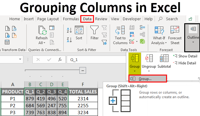
Group Column in Excel means bringing one or more columns together in an Excel worksheet. It enables an option to contract or expand the column, and Excel provides us a button to do so. To group columns, we must select two or more columns, and then from the “Data” tab in the “Outline” section, we have the option to group the columns.
Table of contents
- Excel Column Grouping
- How to Use Column Grouping in Excel? (with Examples)
- Example #1
- Example #2
- How to Hide or Unhide the Group Column?
- Shortcut Keys to Hide or Unhide Column Grouping in Excel
- Why you should use the Excel Column Grouping
- Why you should not use the Excel Column Grouping
- Things to Remember
- Recommended Articles
- How to Use Column Grouping in Excel? (with Examples)
How to Use Column Grouping in Excel? (with Examples)
You can download this Column Grouping Excel Template here – Column Grouping Excel Template
Example #1
Following are the steps of Excel column grouping:
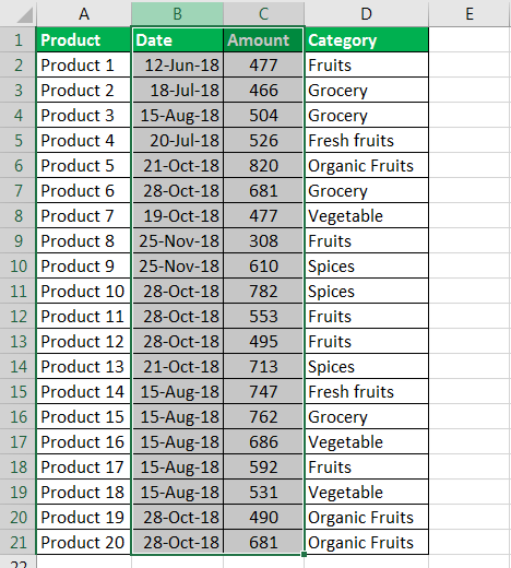
- We must select the data first that we are using to group the column in Excel.

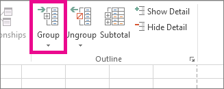
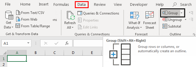
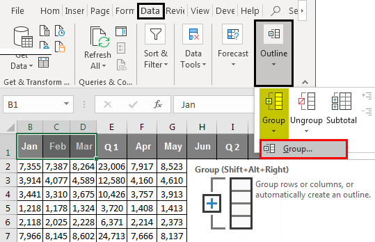
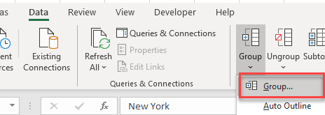
- Then, go to the “Data” option in the Excel toolbar and select the “Group” option in the “Outline” toolbar, as shown in the below screenshot.

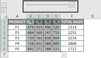
- When we click on the “Group,” it will enable us to group the particular column in the Excel spreadsheet. As shown below in the screenshot, the minus sign symbol is added to the outline above the selected columns.

When we hide columns C and D in a spreadsheet, it is the result. It automatically enables the grouping option in the spreadsheet.


Example #2
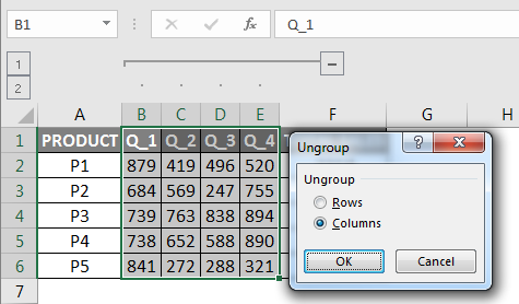
- Step 1: We must first select columns B and C.
- Step 2: Go to the “Data” option in the excel toolbarThe toolbar, also known as the quick access toolbar, is located on the left top-most side of the excel window and has only a few options by default, such as save, redo, and undo. Users can, however, customize it to their liking and add any option or button to make it easier to access the commands.read more and select the “Group” option in the outline toolbar, as shown below.

- Step 3: Next, go to the option group and make the group of a column selected.

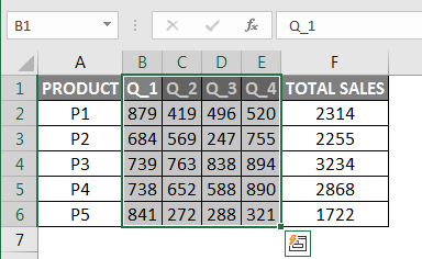
Now, we can see the two minus signs; two groups are created in a particular spreadsheet that we want to group.
How to Hide or Unhide the Group Column?
- Step 1: First, We must click on the created minus sign while grouping the column.

- Step 2: When we click on the minus sign, a column will collapse, resulting in the hide in a column.

- Step 3: Once we click on the minus sign, it automatically shows the plus sign, which means that if we want to unhide the column, click on the plus sign to unhide the columns.
- Step 4: We can likewise utilize the small numbers in the upper left corner. They let us cover up and unhide all groupings of a similar dimension without a moment’s delay. For instance, in the table on the screen capture, clicking on 2 will conceal columns B and D. This is particularly helpful if we made a progressive collection system. Likewise, clicking on 3 will unhide or hide columns C and D.

Shortcut Keys to Hide or Unhide Column Grouping in Excel
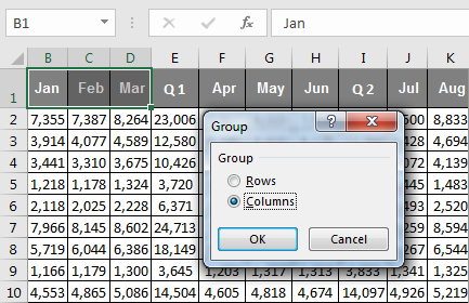
- Step 1: First, we must select the data. Then, press the Shortcut Excel KeysAn Excel shortcut is a technique of performing a manual task in a quicker way.read more – Shift + Alt + right arrow. We may see the dialog box in the Excel spreadsheet as follows:


- Step 2: Select the radio button on a column to hide the columns in excelThe methods to hide columns in excel are — hide columns using right-click option, hide columns using shortcut cut key, hide columns using column width, hide columns using VBA code.read more.

- Step 3: Click on the “OK.” Now, we can hide and unhide the columns in excelUsing the Home tab of the Excel ribbon, using the shortcut key, using the context menu, altering the column width, using the ctrl+G (go to) command, and using the ctrl+F (find) command are some of the ways to unhide a column in Excel.read more.

Why you should use the Excel Column Grouping
- To effectively expand and contract the section or areas of a worksheet.
- To limit schedules or side estimations that different users probably would not require while working in Excel worksheets.
- To keep data composed and in an organized structure.
- To make new sheets (tabs) as a substitute.
- It is a better option than hiding cells.
- It is a better function as compared to hiding the column function.
- It helps to set up the grouping level.
Why you should not use the Excel Column Grouping
- We would not be able to make a group of cells that are not adjacent.
- If we manage different worksheets and need to assemble similar lines/columns on numerous worksheets in the meantime, it is impossible to use this function.
- We always need to check that the data is in a sorted form.
- We always need to check while grouping the column in Excel to select the correct column that needs to group.
Things to Remember
- We would not be able to add the calculated items to grouped fields in the Excel spreadsheet.
- It is impractical to choose a few non-nearby columns.
- Clicking on the minus icon may hide the column, and the icon may change to the plus sign letting us instantly unhide the data.
- We can select the range and press “Shift + Alt + left arrow” to remove the grouping from the Excel spreadsheet.
Recommended Articles
This article is a guide to Group Columns in Excel. We discuss using group Excel columns, examples, and downloadable Excel templates here. You may also look at these useful functions in Excel: –
- Excel Move Columns
- Column Lock in Excel
- Freeze Columns in Excel
- Group Excel Worksheets
Reader Interactions
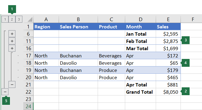
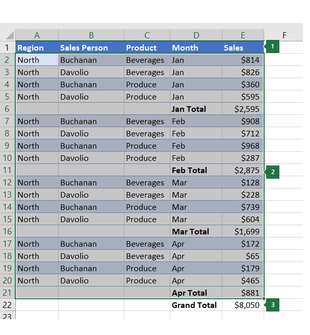
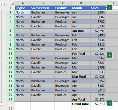
If you have a list of data you want to group and summarize, you can create an outline of up to eight levels. Each inner level, represented by a higher number in the outline symbols, displays detail data for the preceding outer level, represented by a lower number in the outline symbols. Use an outline to quickly display summary rows or columns, or to reveal the detail data for each group. You can create an outline of rows (as shown in the example below), an outline of columns, or an outline of both rows and columns.
|
|
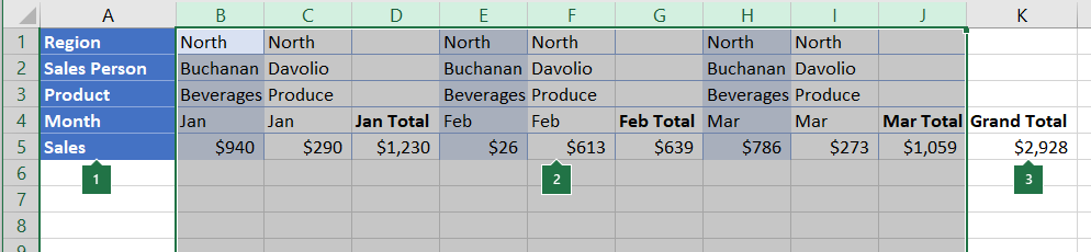
1. To display rows for a level, click the appropriate 2. Level 1 contains the total sales for all detail rows. 3. Level 2 contains total sales for each month in each region. 4. Level 3 contains detail rows — in this case, rows 17 through 20. 5. To expand or collapse data in your outline, click the |
 outline symbols.
 and
and  outline symbols, or press ALT+SHIFT+= to expand and ALT+SHIFT+- to collapse.
-
Make sure that each column of the data that you want to outline has a label in the first row (e.g., Region), contains similar facts in each column, and that the range you want to outline has no blank rows or columns.
-
If you want, your grouped detail rows can have a corresponding summary row—a subtotal. To create these, do one of the following:
-
Insert summary rows by using the Subtotal command
Use the Subtotal command, which inserts the SUBTOTAL function immediately below or above each group of detail rows and automatically creates the outline for you. For more information about using the Subtotal function, see SUBTOTAL function.
-
Insert your own summary rows
Insert your own summary rows, with formulas, immediately below or above each group of detail rows. For example, under (or above) the rows of sales data for March and April, use the SUM function to subtotal the sales for those months. The table later in this topic shows you an example of this.
-
-
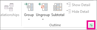
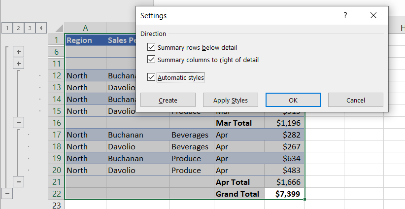
By default, Excel looks for summary rows below the details they summarize, but it’s possible to create them above the detail rows. If you created the summary rows below the details, skip to the next step (step 4). If you created your summary rows above your detail rows, on the Data tab, in the Outline group, click the dialog box launcher.

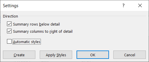
The Settings dialog box opens.
Then in the Settings dialog box, clear the Summary rows below detail checkbox, and then click OK.
-
Outline your data. Do one of the following:
Outline the data automatically
-
Select a cell in the range of cells you want to outline.
-
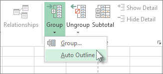
On the Data tab, in the Outline group, click the arrow under Group, and then click Auto Outline.
Outline the data manually
Important: When you manually group outline levels, it’s best to have all data displayed to avoid grouping the rows incorrectly.
-
To outline the outer group (level 1), select all of the rows the outer group will contain (i.e., the detail rows and if you added them, their summary rows).
1. The first row contains labels, and is not selected.
2. Since this is the outer group, select all the rows with subtotals and details.
3. Don’t select the grand total.
-
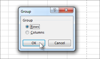
On the Data tab, in the Outline group, click Group. Then in the Group dialog box, click Rows, and then click OK.
Tip: If you select entire rows instead of just the cells, Excel automatically groups by row — the Group dialog box doesn’t even open.
The outline symbols appear beside the group on the screen.
-
Optionally, outline an inner, nested group — the detail rows for a given section of your data.
Note: If you don’t need to create any inner groups, skip to step f, below.
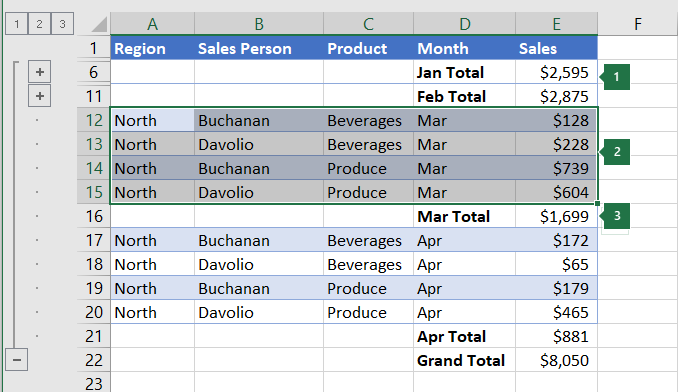
For each inner, nested group, select the detail rows adjacent to the row that contains the summary row.
1. You can create multiple groups at each inner level. Here, two sections are already grouped at level 2.
2. This section is selected and ready to group.
3. Don’t select the summary row for the data you are grouping.
-
On the Data tab, in the Outline group, click Group.
Then in the Group dialog box, click Rows, and then click OK. The outline symbols appear beside the group on the screen.
Tip: If you select entire rows instead of just the cells, Excel automatically groups by row — the Group dialog box doesn’t even open.
-
Continue selecting and grouping inner rows until you have created all of the levels that you want in the outline.
-
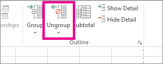
If you want to ungroup rows, select the rows, and then on the Data tab, in the Outline group, click Ungroup.
You can also ungroup sections of the outline without removing the entire level. Hold down SHIFT while you click the
or for the group, and then on the Data tab, in the Outline group, click Ungroup.Important: If you ungroup an outline while the detail data is hidden, the detail rows may remain hidden. To display the data, drag across the visible row numbers adjacent to the hidden rows. Then on the Home tab, in the Cells group, click Format, point to Hide & Unhide, and then click Unhide Rows.
-
-
Make sure that each row of the data that you want to outline has a label in the first column, contains similar facts in each row, and the range has no blank rows or columns.
-
Insert your own summary columns with formulas immediately to the right or left of each group of detail columns. The table listed in step 4 below shows you an example.
Note: To outline data by columns, you must have summary columns that contain formulas that reference cells in each of the detail columns for that group.
-
If your summary column is to the left of the detail columns, on the Data tab, in the Outline group, click the dialog box launcher.
The Settings dialog box opens.
Then in the Settings dialog box, clear the Summary columns to right of detail check box, and click OK.
-
To outline the data, do one of the following:
Outline the data automatically
-
Select a cell in the range.
-
On the Data tab, in the Outline group, click the arrow below Group and click Auto Outline.
Outline the data manually
Important: When you manually group outline levels, it’s best to have all data displayed to avoid grouping columns incorrectly.
-
To outline the outer group (level 1), select all of the subordinate summary columns, as well as their related detail data.
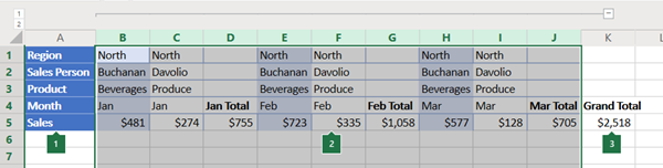
1. Column A contains labels.
2. Select all the detail and subtotal columns. Note that if you don’t select entire columns, when you click Group (on the Data tab in the Outline group) the Group dialog box will open and ask you to choose Rows or Columns.
3. Don’t select the grand total column.
-
On the Data tab, in the Outline group, click Group.
The outline symbol appears above the group.
-
To outline an inner, nested group of detail columns (level 2 or higher), select the detail columns adjacent to the column that contains the summary column.
1. You can create multiple groups at each inner level. Here, two sections are already grouped at level 2.
2. These columns are selected and ready to group. Note that if you don’t select entire columns, when you click Group (on the Data tab in the Outline group) the Group dialog box will open and ask you to choose Rows or Columns.
3. Don’t select the summary column for the data you are grouping.
-
On the Data tab, in the Outline group, click Group.
The outline symbols appear beside the group on the screen.
-
-
Continue selecting and grouping inner columns until you have created all of the levels that you want in the outline.
-
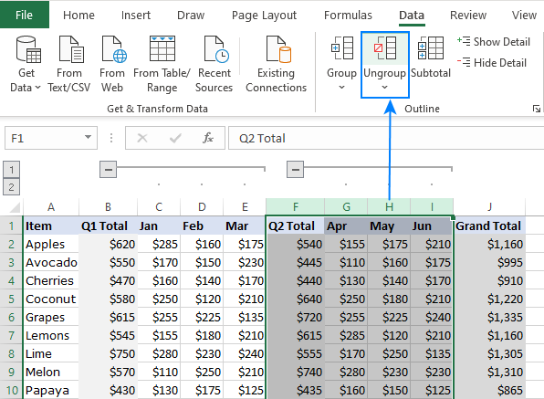
If you want to ungroup columns, select the columns, and then on the Data tab, in the Outline group, click Ungroup.
You can also ungroup sections of the outline without removing the entire level. Hold down SHIFT while you click the  or
or  for the group, and then on the Data tab, in the Outline group, click Ungroup.
If you ungroup an outline while the detail data is hidden, the detail columns may remain hidden. To display the data, drag across the visible column letters adjacent to the hidden columns. On the Home tab, in the Cells group, click Format, point to Hide & Unhide, and then click Unhide Columns
-
If you don’t see the outline symbols
, , and , go to File > Options > Advanced, and then under the Display options for this worksheet section, select the Show outline symbols if an outline is applied check box, and then click OK. -
Do one or more of the following:
-
Show or hide the detail data for a group
To display the detail data within a group, click the
button for the group, or press ALT+SHIFT+=. -
To hide the detail data for a group, click the
button for the group, or press ALT+SHIFT+-. -
Expand or collapse the entire outline to a particular level
In the
outline symbols, click the number of the level that you want. Detail data at lower levels is then hidden.For example, if an outline has four levels, you can hide the fourth level while displaying the rest of the levels by clicking
. -
Show or hide all of the outlined detail data
To show all detail data, click the lowest level in the
outline symbols. For example, if there are three levels, click . -
To hide all detail data, click
.
-
 .
. .
.For outlined rows, Microsoft Excel uses styles such as RowLevel_1 and RowLevel_2 . For outlined columns, Excel uses styles such as ColLevel_1 and ColLevel_2. These styles use bold, italic, and other text formats to differentiate the summary rows or columns in your data. By changing the way each of these styles is defined, you can apply different text and cell formats to customize the appearance of your outline. You can apply a style to an outline either when you create the outline or after you create it.
Do one or more of the following:
Automatically apply a style to new summary rows or columns
-
On the Data tab, in the Outline group, click the dialog box launcher.
The Settings dialog box opens.
-
Select the Automatic styles check box.
Apply a style to an existing summary row or column
-
Select the cells to which you want to apply a style.
-
On the Data tab, in the Outline group, click the dialog box launcher.
The Settings dialog box opens.
-
Select the Automatic styles check box, and then click Apply Styles.
You can also use autoformats to format outlined data.
-
If you don’t see the outline symbols
, , and , go to File > Options > Advanced, and then under the Display options for this worksheet section, select the Show outline symbols if an outline is applied check box. -
Use the outline symbols
, , and to hide the detail data that you don’t want copied.For more information, see the section, Show or hide outlined data.
-
Select the range of summary rows.
-
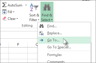
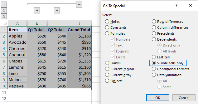
On the Home tab, in the Editing group, click Find & Select, and then click Go To.
-
Click Go To Special.
-
Click Visible cells only.
-
Click OK, and then copy the data.
Note: No data is deleted when you hide or remove an outline.
Hide an outline
-
Go to File > Options > Advanced, and then under the Display options for this worksheet section, uncheck the Show outline symbols if an outline is applied check box.
Remove an outline
-
Click the worksheet.
-
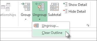
One the Data tab, in the Outline group, click Ungroup and click Clear Outline.
Important: If you remove an outline while the detail data is hidden, the detail rows or columns may remain hidden. To display the data, drag across the visible row numbers or column letters adjacent to the hidden rows and columns. On the Home tab, in the Cells group, click Format, point to Hide & Unhide, and then click Unhide Rows or Unhide Columns.
Imagine that you want to create a summary report of your data that only displays totals accompanied by a chart of those totals. In general, you can do the following:
-
Create a summary report
-
Outline your data.
For more information, see the sections Create an outline of rows or Create an outline of columns.
-
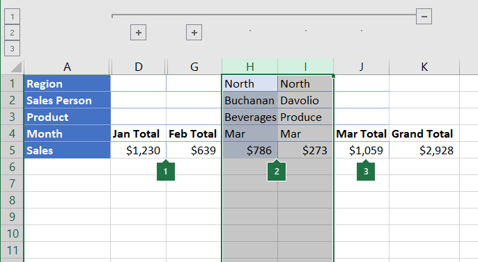
Hide the detail by clicking the outline symbols
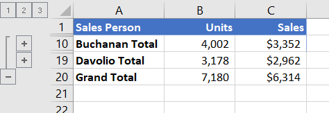
, , and to show only the totals as shown in the following example of a row outline:
-
For more information, see the section, Show or hide outlined data.
-
-
Chart the summary report
-
Select the summary data that you want to chart.
For example, to chart only the Buchanan and Davolio totals, but not the grand totals, select cells A1 through C19 as shown in the above example.
-
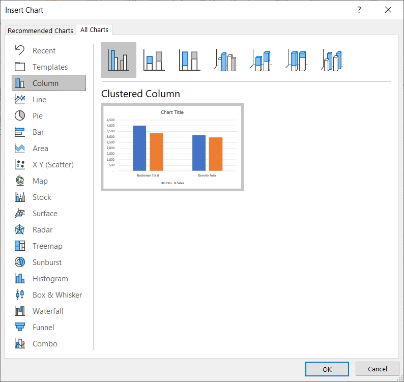
Click Insert > Charts > Recommended Charts, then click the All Charts tab and choose your chart type.
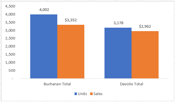
For example, if you chose the Clustered Column option, your chart would look like this:
If you show or hide details in the outlined list of data, the chart is also updated to show or hide the data.
-
You can group (or outline) rows and columns in Excel for the web.
Note: Although you can add summary rows or columns to your data (by using functions such as SUM or SUBTOTAL), you cannot apply styles or set a position for summary rows and columns in Excel for the web.
Create an outline of rows or columns
|
|
|
|
Outline of rows in Excel Online
|
Outline of columns in Excel Online
|
-
Make sure that each column (or row) of the data that you want to outline has a label in the first row (or column), contains similar facts in each column (or row), and that the range has no blank rows or columns.
-
Select the data (including any summary rows or columns).
-
On the Data tab, in the Outline group, click Group > Group Rows or Group Columns.
-
Optionally, if you want to outline an inner, nested group — select the rows or columns within the outlined data range, and repeat step 3.
-
Continue selecting and grouping inner rows or columns until you have created all of the levels that you want in the outline.
Ungroup rows or columns
-
To ungroup, select the rows or columns, and then on the Data tab, in the Outline group, click Ungroup and select Ungroup Rows or Ungroup Columns.
Show or hide outlined data
Do one or more of the following:
Show or hide the detail data for a group
-
To display the detail data within a group, click the
for the group, or press ALT+SHIFT+=. -
To hide the detail data for a group, click the
for the group, or press ALT+SHIFT+-.
Expand or collapse the entire outline to a particular level
-
In the
outline symbols, click the number of the level that you want. Detail data at lower levels is then hidden. -
For example, if an outline has four levels, you can hide the fourth level while displaying the rest of the levels by clicking
.
Show or hide all of the outlined detail data
-
To show all detail data, click the lowest level in the
outline symbols. For example, if there are three levels, click . -
To hide all detail data, click
.
Need more help?
You can always ask an expert in the Excel Tech Community or get support in the Answers community.
See Also
Group or ungroup data in a PivotTable
Grouping Columns in Excel (Table of Content)
- Excel Grouping Columns
- How to Enable Grouping of Columns in Excel?
Excel Grouping Columns
Sometimes the worksheet contains complex data, which is very difficult to read & analyze, to Access & read these types of data in an easier way, the grouping of cells will help you out. Grouping of columns or rows is used if you want to visually group of items or to monitor them in a concise & organized manner under one heading or if you want to hide or show data for better display & presentation. Grouping is very useful & most commonly used in accounting & finance spreadsheets. Under the Data tab in the Ribbon, you can find the Group option in the outline section. In this topic, we are going to learn about Grouping Columns in Excel.
Shortcut Key to Group Columns or Rows
Shift+Alt+Right Arrow is the shortcut key to group columns or rows, whereas
Shift+Alt+Left Arrow is the shortcut key to ungroup columns or rows.
Definition Grouping of Columns in Excel
It’s a process where you visually group the column items or datasets for a better display.
How to Enable Grouping of Columns in Excel?
Let’s check out how to group columns & How to collapse & expand columns after grouping columns.
You can download this Grouping Columns Excel Template here – Grouping Columns Excel Template
Example #1 – Grouping of Columns in Excel
Grouping of columns in Excel works out well for structured data where it should contain column headings, and it should not have a blank column or row data.
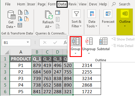
Initially, you need to select the column in which you want to group it (i.e. B, C, D, E columns). Go to the Data tab, then click on the group option under the outline section.
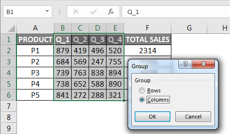
Click on the columns and then press OK.
Now you can observe in data, the columns are grouped perfectly, and the outline bars you can observe at the top represent different levels of data organization. Grouping also introduces a toggle option, or it will create a hierarchy of groups, which is known as an outline, to help your worksheet appear in an organized manner, where each bar represents a level of organization (Grouping is also referred to as Outlines.)
How to Collapse & Expand Columns After Column Grouping
you can press the “-” buttons in the margin to collapse the columns (B, C, D, E Columns completely disappears) or in case If you want to expand them again, press the “+” buttons in the margin (B, C, D, E Columns appears)
Another way to access data is the use of 1 or 2 options on the left side of the worksheet, i.e. it is called a state, 1st option is called a hidden state (if you click on it, it will hide B, C, D, E Columns) whereas 2nd option is called unhidden state, it will expand those hidden columns, I.E. B, C, D, E Columns appears
To Ungroup Columns in Excel
Select the columns you wish to ungroup (i.e. the columns which you have previously grouped). On the Data tab, in the Outline group, click on Ungroup command.
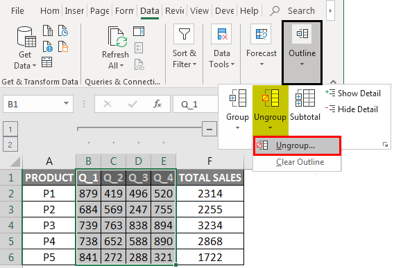
Click on the columns and then press OK.
Now, you can observe data bars & “+” buttons and “-” buttons disappear in the excel sheet once the ungroup option is selected.
Example #2 – Multiple Grouping of Columns for Sales Data in Excel
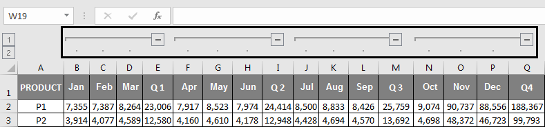
In the below-mentioned example, the Table contains product monthly sales data from Jan to Dec month, and it is also represented in quarterly & yearly sales.
Here the data is structured and does not contain any blank cells, hidden rows, or columns.
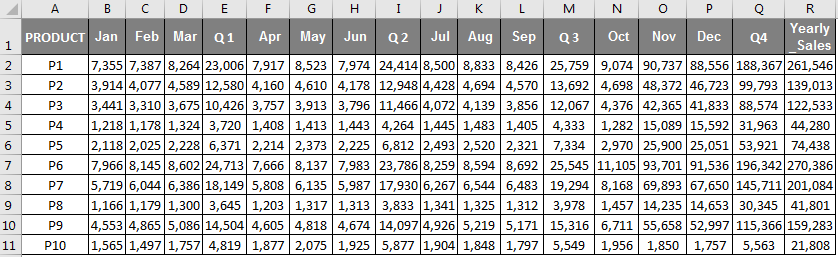
I don’t want all the monthly sales data to be displayed; I want only quarterly & yearly sales data to be displayed; it can be done through multiple grouping of column options.
Initially, I need to select the column which I want to group it; now, let’s select the months (i.e. Jan, Feb, Mar columns). Go to the Data tab in the Home ribbon, and it will open a toolbar below the ribbon, then click on the group option under the outline section; now you can observe in a data, the columns are grouped perfectly.
Click on the columns and then press OK.
A similar procedure is applied or followed for the month of Apr, May, Jun & Jul, Aug, Sep & Oct, Nov, Dec columns.
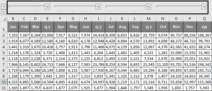
Once the grouping of the above-mentioned monthly columns is done, you can observe that the columns are grouped perfectly in a dataset. The four outline bars you can observe at the top represent different data organisation levels.
Collapsing & Expanding Columns After Column Grouping
You can press the “–” symbol or buttons in the outline bar to collapse all the month columns; once you are done, you can observe all the month Columns completely disappears, and Positive or “+” buttons in the outline bar appear.

Now, the sales data looks in a concise & compact form, and it looks well-organized & structured financial data. In case if you want to check any specific monthly sales data, you can expand them again by pressing the “+” buttons in in outline bar so that again, all the monthly sales data will appear.
Another way to access or hide monthly data is the use of 1 or 2 options on the left side of the worksheet, i.e. it is called a state, 1st option is called a hidden state (On a single click on it, it will hide all the month Columns) whereas 2nd option is called unhidden state, it will expand those hidden columns, I.E. all the month Columns appears.
Things to Remember
Grouping columns or rows in Excel is useful to create and maintain well-organized and well-structured financial sales data.
It is a better & superior alternative for hiding & unhiding cells; sometimes, it is not clear to the other user of the excel spreadsheet if you use the hide option. He needs to track which columns or rows you have hidden & where you have hidden.
Prior to applying grouping of columns or rows in excel, You have to ensure that your structured data should not contain any hidden or blank rows & columns; otherwise, your data will be grouped incorrectly.
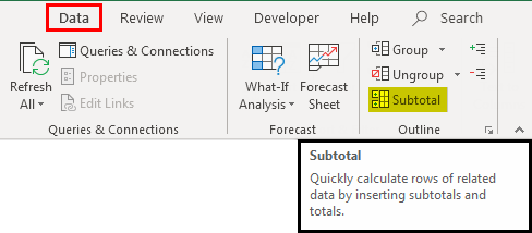
Apart from grouping, you can also do summarization of datasets in different groups with the help of the Subtotal command.
Recommended Articles
This has been a guide to Grouping Columns in Excel. Here we discussed How to Enable Grouping of Columns in Excel along with Examples and a downloadable excel template. You may also look at these useful functions in excel –
- Excel Move Columns
- VBA Columns
- Freeze Columns in Excel
- Switching Columns in Excel
When working on an extensive Excel worksheet, you can avoid getting confused and overwhelmed by organizing columns into groups.
This will enable you to easily show and hide different areas of the worksheet so that only relevant data is visible.
In this tutorial, I will show you three methods to group columns in Excel.
Note: Ensure that the worksheet does not have any hidden columns before applying any of the following methods.
Method #1: Select the Columns to be Grouped and Apply the Group Command
When we use this method, we first select the columns that we want to group and then apply the Group command.
The following dataset shows the sales of various tablets for three quarters.

In the above dataset, I want to group all the columns between the Tablet column and the Grand Total Column (so that all the months and quarters sales data could be easily hidden with a click).
Below are the steps to group columns in Excel:
- Select the columns by clicking the header of column B, holding down the mouse button, and dragging across the column headers to the header of column M.

- Select the Data tab, in the Outline group, click the downward arrow on the Group button and choose the Group option.

Alternatively, you can use the keyboard shortcut Shift + Alt + Right Arrow.
Level 1 outline is created as shown below (a gray line appears over the columns that have been grouped):

When you click the outline number 1 button in the top left corner (or you click the minus button in the top right corner), all the columns within the group are hidden, as shown below:

To unhide the columns, click the plus (+) button on top of the group.
How to Create Inner Groups
In the above example, we have created only one outline where all the selected columns were grouped.
Now you can follow the same steps and create inner groups within the main group.
For example, in our data set, we have grouped all the month’s data together as the main outline, and then we can also create inner groups for each quarter.
Below is our dataset where we have a Level 1 outline where all the columns in between columns A and N are grouped.

We want to create an inner group of columns within this group.
Below are the steps to create an inner group of columns:
- Select the columns we want to be included in the inner group. We want to include columns B, C, and D in this case.

- Select the Data tab, in the Outline group, click the downward arrow on the Group button and choose the Group option.

Alternatively, you can use the keyboard shortcut Shift + Alt + Right Arrow.
The inner group is created:

Note that because only adjacent columns can be grouped, we will have to repeat the process for any other group we want to create.
We can group the three columns preceding the Q2 Total column and the three columns preceding the Q3 Total column in the same way.

We now have 2 levels of column groups:
- One outer level 1 group is made up of columns B to M.
- Three inner level 2 groups; columns B-D, columns E-H, and columns J-K.
To collapse all the inner groups, click the level 2 button on the left of the groups.

To collapse each inner group click the minus (-) button on top of the group.
Method #2: Select Cells in the Columns to be Grouped and Apply the Group Command
This method is a variation of Method #1.
Instead of selecting the columns to be grouped and then applying the Group command, we select cells in the columns we want to group and apply the Group command.
The following dataset shows the sales of various tablets for three quarters.

We want to group all the columns between the Tablet and the Grand Total column.
Below are the steps to group columns in Excel:
- Select at least one cell in the columns we want to group.

- Select the Data tab, in the Outline group, click the downward arrow on the Group button and choose the Group option.

Alternatively, you can use the keyboard shortcut Shift + Alt + Right Arrow.
- In the Group dialog box that opens, select the Columns option and hen click Ok.

Level 1 outline is created as shown below:

Once the outline has been created, you can quickly hide the columns by clicking on the minus button at the top right part of the worksheet (the minus button is at the end of the gray line).
As soon as you click on the minus button, all the columns you have grouped will be hidden, and you will get the result as shown below.

To unhide the columns click the plus (+) button on top of the group.
Method #3: Use the Auto Outline Option
If your dataset has a predictable pattern, you can use the Auto Outline option in the Outline group to group the columns automatically.
The following dataset has a predictable pattern.

Columns B, C, D, F, G, H, J, K, and L contain the same type of data, the monthly sales figures for various tablets.
Each of the columns E, I, and M contains the summation of the three preceding columns. Column N contains the Grand Total of columns E, I, and M.
We can easily group columns in this dataset using the Auto Outline option.
We use the following steps to group the columns between the Tablet column and the Grand Total column.
- Select the tab of the worksheet containing the dataset to activate the worksheet.
- Select the Data tab, in the Outline group, click the down arrow on the Group button and choose the Auto Outline option.

Levels 1 and 2 outlines are created as shown below:

The columns of the dataset have been grouped into one level 1 outline and three level 2 outlines. There are three level 2 outlines because the data represents the tablet sales for three quarters.
When you click the outline number 1 button in the top left corner (or the minus button in the top right corner at the end of the gray line), all the columns within the group are hidden, as shown below:

We can unhide the columns or expand the group by clicking the plus (+) button on top of the group.
To hide the months in groups of threes, click on the minus (-) buttons of the level 2 outline.
In the following example, we have clicked the first minus (-) button of the level 2 outline to hide the first three months:

To collapse all the level 2 groups, we click the level number 2 button on the left of the outline area:

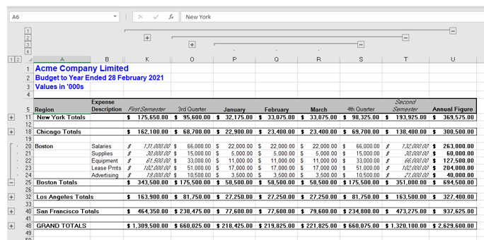
How to Group Columns When Summary Columns are On the Right of Detail Columns
Sometimes your dataset may have the summary columns on the left of the detail columns, as shown below:

You need to do the following before using the Auto Outline feature:
- Click the dialog box launcher icon in the bottom right corner of the Outline group.

- In the Settings dialog box that appears, deselect the ‘Summary columns to right of detail‘ option and click OK.

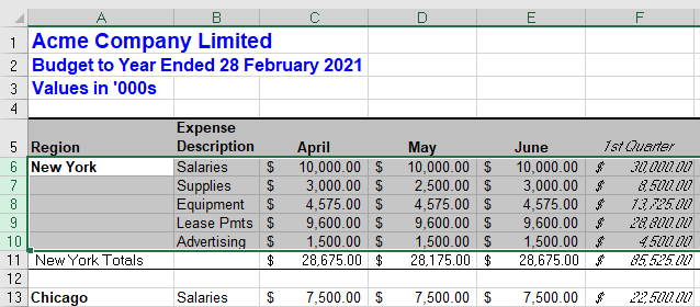
You can now use the Auto Outline option as explained earlier in this method, and the result will be as follows:

Notice that the Auto Outline feature has generated only one level of grouping with three groups, and the minus (-) buttons are on the left of the groups and not on the right.
How to Ungroup Particular Columns
To ungroup particular columns do the following:
- Select the columns you want to ungroup, for example, columns B-D in the following dataset,

- On the Data tab, in the Outline group, click the Ungroup button.

Alternatively, you can use the shortcut Shift + Alt + Left Arrow Key.
Columns B-D are ungrouped as seen below:

How to Clear an Outline in Grouped Columns
To remove all the column groupings, do the following:
- Open the Data tab, in the Outline group, click the down arrow below the Ungroup button and choose the Clear Outline option.

The other steps would instantly remove the outline in all the column groupings would be gone.
In this tutorial, I covered some methods you can use to group columns in Excel quickly.
If your data is arranged where there’s a predictable pattern, you can use the Auto Outline option, which would automatically create one or more levels of grouping for your data set.
You can also manually select the columns (or the cells in the columns you want to group) and then group them using the options in the ribbon.
Other Excel articles you may also like:
- How to Group Worksheets in Excel
- How to Group Numbers in Pivot Table in Excel
- Create Groups in Quick Access Toolbar in Excel
- How to Freeze Multiple Columns in Excel?
- Delete Blank Columns in Excel (3 Easy Ways + VBA)
- Select Till End of Data in a Column in Excel (Shortcuts)
- How to Delete All Hidden Rows and Columns in Excel
- How to Quickly Unhide COLUMNS in Excel (A Simple Guide)
Содержание
- How to Group in Excel
- In This Article
- Grouping in Excel
- How to Use Excel to Group Rows Manually
- How to Manually Group Columns in Excel
- How to Make Excel Group Columns and Rows Automatically
- How to Create a Multi-Level Group Hierarchy in Excel
- How to Automatically Create Multi-Level Hierarchy
- How to Expand and Collapse Groups
- Group in Excel
- Guide on How to Group in Excel
- Keyboard Shortcuts Sheet
- Excel Group Function
- Example of How to Group in Excel
- Why You Should Never Hide Cells in Excel
- Download Excel Group Template
- Additional Resources
- How to group columns in Excel
- How to group columns in Excel
- Create nested column groups
- How to auto outline columns in Excel
- How to hide and show grouped columns
- Hide and show a particular column group
- Expand or collapse the whole outline to a given level
- Hide and show all of the grouped data
- How to copy only visible columns
- How to ungroup columns in Excel
- How to remove the entire outline
- How to ungroup specific columns
How to Group in Excel
Get a handle on your data
:max_bytes(150000):strip_icc()/JodyMuelaner-6e62f52047f044b08c84c2b87fbeebea.jpg)
In This Article
Jump to a Section
Grouping rows and columns in Excel lets you collapse and expand sections of a worksheet. This can make large and complex datasets much easier to understand. Views become compact and organized. This article shows you step-by-step how to group and view your data.
Instructions in this article apply to Excel 2019, 2016, 2013, 2010, 2007; Excel for Microsoft 365, Excel Online and Excel for Mac.
Grouping in Excel
You can create groups by either manually selecting the rows and columns to include, or you can get Excel to automatically detect groups of data. Groups can also be nested inside other groups to create a multi-level hierarchy. Once your data is grouped, you can individually expand and collapse groups, or you can expand and collapse all groups at a given level in the hierarchy.
Groups provide a really useful way to navigate and view large and complex spreadsheets. They make it much easier to focus on the data that’s important. If you need to make sense of complex data you should definitely be using Groups and could also benefit from Power Pivot For Excel.
:max_bytes(150000):strip_icc()/15-Mixed-levels-da647df23db24f94ac2ca0f10e375c06.jpg)
How to Use Excel to Group Rows Manually
To make Excel group rows, the simplest method is to first select the rows you want to include, then make them into a group.
For the group of rows you want to group, select the first row number and drag down to the last row number to select all the rows in the group.
:max_bytes(150000):strip_icc()/001_how-to-group-in-excel-7b0153797bb344b88a4b47c7b54e7471.jpg)
Select the Data tab > Group > Group Rows, or simply select Group, depending on which version of Excel you’re using.
:max_bytes(150000):strip_icc()/002_how-to-group-in-excel-0438eb26a99b4a5fbd4988c108905cb5.jpg)
A thin line will appear to the left of the row numbers, indicating the extent of the grouped rows.
:max_bytes(150000):strip_icc()/003_how-to-group-in-excel-25021e1028884370a574f4dd7940fc8e.jpg)
Select the minus (-) to collapse the group. Small boxes containing the numbers one and two also appear at the top of this region, indicating the worksheet now has two levels in its hierarchy: the groups and the individual rows within the groups.
The rows have been grouped and can now be collapsed and expanded as required. This makes it much easier to focus on just the relevant data.
How to Manually Group Columns in Excel
To make Excel group columns, the steps are almost the same as doing so for rows.
For the group of columns you want to group, select the first column letter and drag right to the last column letter, thereby selecting all the columns in the group.
:max_bytes(150000):strip_icc()/004_how-to-group-in-excel-d6164b87c8aa44d88615ebe482bc217a.jpg)
Select the Data tab > Group > Group Columns, or select Group, depending on which version of Excel you’re using.
:max_bytes(150000):strip_icc()/005_how-to-group-in-excel-b4daa44acc5f46548bf0b5a5f6b02350.jpg)
A thin line will appear above the column letters. This line indicates the extent of the grouped columns.
:max_bytes(150000):strip_icc()/006_how-to-group-in-excel-bb3cb070500f4033be83eae7f428485a.jpg)
Select the minus (-) to collapse the group. Small boxes containing the numbers one and two also appear at the top of this region, indicating the worksheet now has two levels in its hierarchy for columns, as well as for rows.
The rows have been grouped and can now be collapsed and expanded as required.
How to Make Excel Group Columns and Rows Automatically
While you could repeat the above steps to create each group in your document, Excel can automatically detect groups of data and do it for you. Excel creates groups where formulas reference a continuous range of cells. If your worksheet doesn’t contain any formulas, Excel won’t be able to automatically create groups.
:max_bytes(150000):strip_icc()/007_how-to-group-in-excel-8fa872f54f764f9eb0e8e9b79b730c3a.jpg)
Select the Data tab > Group > Auto Outline and Excel will create the groups for you. In this example, Excel correctly identified each of the groups of rows. Because there’s no annual total for each spending category, it has not automatically grouped the columns.
:max_bytes(150000):strip_icc()/08-Auto-Grouped-866b0020299e48739c3c506fc9ae9512.jpg)
This option isn’t available in Excel Online, if you’re using Excel Online, you’ll need to create groups manually.
How to Create a Multi-Level Group Hierarchy in Excel
In the previous example, categories of income and expense were grouped together. It would make sense to also group all of the data for each year. You can do this manually by applying the same steps as you used to create the first level of groups.
Select all of the rows to be included.
:max_bytes(150000):strip_icc()/008_how-to-group-in-excel-70a5edaa206d4494a10bbd53517199b7.jpg)
Select the Data tab > Group > Group Rows, or select Group, depending on which version of Excel you are using.
Another thin line will appear to the left of the lines representing the existing groups and indicating the extent of the new group of rows. The new group encompasses two of the existing groups and there are now three small numbered boxes at the top of this region, signifying the worksheet now has three levels in its hierarchy.
:max_bytes(150000):strip_icc()/009_how-to-group-in-excel-a6245c3696b24c47be33dcfb4cd509c1.jpg)
The spreadsheet now contains two levels of groups, with individual rows within the groups.
How to Automatically Create Multi-Level Hierarchy
Excel uses formulas to detect multi-level groups, just as it uses them to detect individual groups. If a formula references more than one of the other formulas which define groups, this indicates these groups are part of a parent group.
:max_bytes(150000):strip_icc()/11-Auto-multi-level-f27cede739e446c3a778ae13ae473a34.jpg)
Keeping with the cash flow example, if we add a Gross Profit row to each year, which is simply the income minus the expenses, then this allows Excel to detect that each year is a group and the income and expenses are sub-groups within these. Select the Data tab > Group > Auto Outline to automatically create these multi-level groups.
How to Expand and Collapse Groups
The purpose of creating these groups of rows and/or columns is that it allows regions of the spreadsheet to be hidden, providing a clear overview of the entire spreadsheet.
To collapse all of the rows, select the number 1 box at the top of the region to the left of the row numbers.
:max_bytes(150000):strip_icc()/010_how-to-group-in-excel-209f6c1ff4864f598ff604cd2f9ab67b.jpg)
Select the number two box to expand the first level of groups and make the second level of groups visible. The individual rows within the second level groups remain hidden.
:max_bytes(150000):strip_icc()/011_how-to-group-in-excel-d2ed9216ebea41a7bf22a76205bfa890.jpg)
Select the number three box to expand the second level of groups so the individual rows within these groups also become visible.
:max_bytes(150000):strip_icc()/012_how-to-group-in-excel-027509f1fef745cf8d5c3cfd641b437c.jpg)
It’s also possible to expand and collapse individual groups. To do so, select the Plus (+) or Minus (-) that appears to mark a group that’s either collapsed or expanded. In this way, groups at different levels in the hierarchy can be viewed as required.
Источник
Group in Excel
The best way to keep spreadsheets organized
Guide on How to Group in Excel
Grouping rows and columns in Excel[1] is critical for building and maintaining a well-organized and well-structured financial model. Using the Excel group function is the best practice when it comes to staying organized, as you should never hide cells in Excel. This guide will show you how to group in Excel with step-by-step instructions, examples, and screenshots.

Keyboard Shortcuts Sheet
Looking to be an Excel wizard? Increase your productivity with CFI’s comprehensive keyboard shortcuts guide.
Excel Group Function
The Excel group function is one of the best secrets a world-class financial analyst uses to make their work extremely organized and easy for other users of the spreadsheet to understand.
Reasons to use the Excel Group Function:
- To easily expand and contract sections of a worksheet
- To minimize schedules or side calculations that other users might not need
- To keep information organized
- As a substitute for creating new sheets (tabs)
- As a superior alternative to hiding cells
The function is found in the Data section of the Ribbon, then Group.
Example of How to Group in Excel
Let’s look at a simple exercise to see how it works. Suppose we have a schedule in a worksheet that is becoming quite long, and we want to reduce the amount of detail that’s shown. The screenshots below will show you how to properly implement grouping in Excel.
Here are the steps to follow to group rows:
- Select the rows you wish to add grouping to (entire rows, not just individual cells)
- Go to the Data Ribbon
- Select Group
- Select Group again
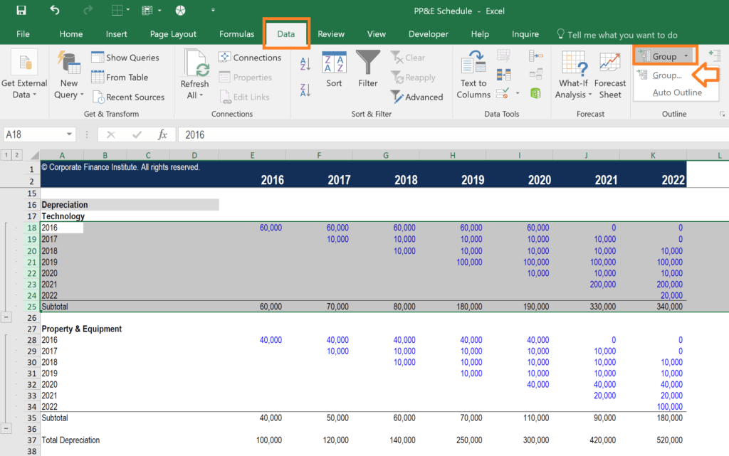
You can repeat the steps above as many times as you like, and you can also apply it to columns as well.
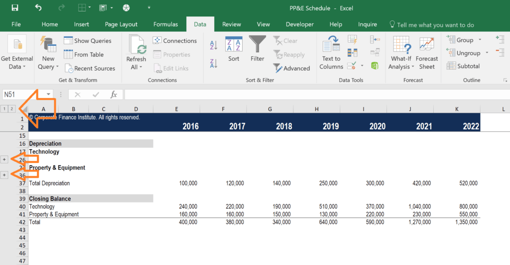
Once you’re finished, you can press the “-” buttons in the margin to collapse the rows or columns.
If you want to expand them again, press the “+” buttons in the margin, as shown in the screenshot below.
There is also a “1” button in the top left corner to collapse all groups, and a “2” button to expand all groups.
Why You Should Never Hide Cells in Excel
Though many people do it, you should never hide cells in Excel (or spreadsheets either, for that matter). The reason is that Excel does not make it clear to the user of the spreadsheet that cells have been hidden, and thus they may go unnoticed.
The only way to see that cells are hidden is to notice that the row number or column number suddenly jumps (e.g., from row 25 to row 167).
Since other users of the spreadsheet may not notice this (and you may forget yourself) you should never hide cells in Excel.
Download Excel Group Template
You can download the Template for free if you wish to use it as an example or starting point for how to group in Excel and apply it to your own work and financial analysis.
Additional Resources
Thank you for reading CFI’s guide to Group in Excel. To continue learning and advancing your career, these additional CFI resources will be helpful:
Источник
How to group columns in Excel
 by Alexander Frolov, updated on March 7, 2023
The tutorial looks at how to group columns in Excel manually and use the Auto Outline feature to group columns automatically.
If you feel overwhelmed or confused about the extensive content of your worksheet, you can organize columns in groups to easily hide and show different parts of your sheet, so that only the relevant information is visible.
How to group columns in Excel
When grouping columns in Excel, it’s best to do this manually because the Auto Outline feature often delivers controversial results.
Note. To avoid incorrect grouping, make sure your worksheet does not have any hidden columns.
To group columns in Excel, perform these steps:
- Select the columns you want to group, or at least one cell in each column.
- On the Data tab, in the Outline group, click the Group button. Or use the Shift + Alt + Right Arrow shortcut.
- If you’ve selected cells rather than entire columns, the Group dialog box will appear asking you to specify exactly what you want grouped. Obviously, you choose Columns and click OK.

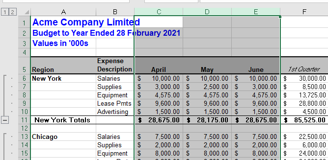
To see how it works in practice, let’s group all the intermediate columns in the below dataset. For this, we highlight columns B through I, and click Group: 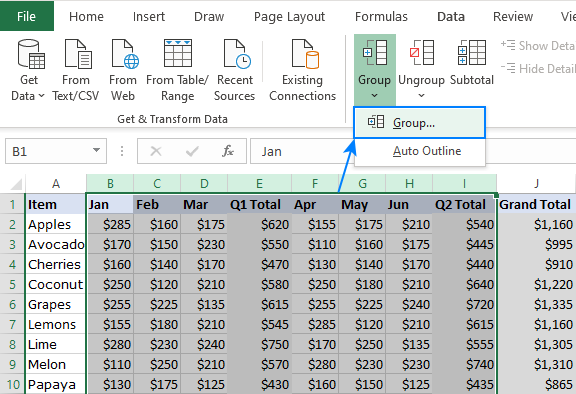
This creates the level 1 outline like shown below: 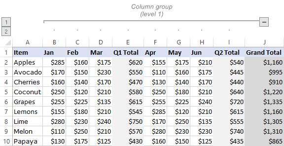
Clicking the minus (-) sign at the top of the group or the outline number 1 in the upper-left corner hides all the columns within the group: 
Create nested column groups
Within any group, you can outline multiple groups at inner levels. To create an inner, nested group of columns, this is what you need to do:
- Select the columns to be included in the inner group.
- On the Data tab, in the Outline group, click Group. Or press the Shift + Alt + Right Arrow shortcut.
In our dataset, to group the Q1 details, we select columns B through D and click Group: 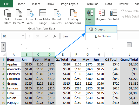
In the same fashion, you can group Q2 details (columns F through H).
Note. As only adjacent columns can be grouped, you will have to repeat the above steps for each inner group individually.
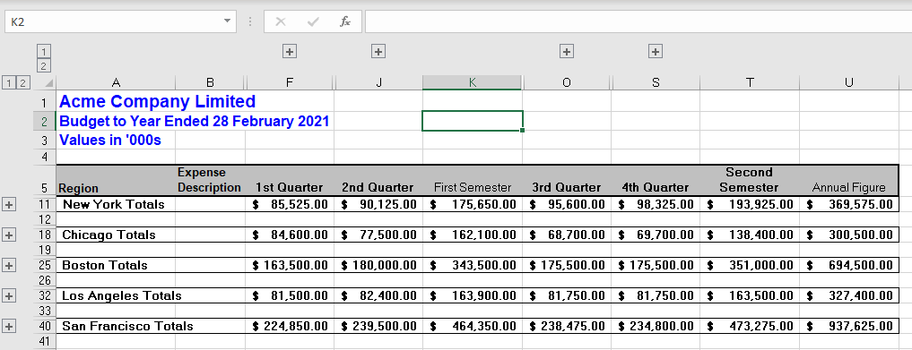
As the result, we now have 2 levels of grouping:
- Outer group (level 1) — columns B through I
- Two inner groups (level 2) — columns B — D and F — H.
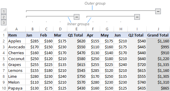
Clicking the minus (-) button above the inner group contracts only that particular group. Clicking the number 2 in the upper-left corner collapses all the groups of this level: 
To make the hidden data visible again, expand the column group by clicking the plus (+) button. Or you can expand all the groups at a given level by clicking the outline number.
- To quickly hide or show the outline bars and numbers, press the Ctrl + 8 keys together. Pressing the shortcut for the first time hides the outline symbols, pressing it again redisplays the outline.
- If the outline symbols don’t show up in your Excel, make sure the Show outline symbols if an outlineis applied check box is selected in your settings: File tab >Options >Advanced category.
How to auto outline columns in Excel
Microsoft Excel can also create an outline of columns automatically. This works with the following caveats:
- There should be no blank columns in your dataset. If there are any, remove them as described in this guide.
- To the right of each group of detail columns, there should be a summary column with formulas.
In our dataset, there are 3 summary columns like show below: 
To auto outline columns in Excel, do the following:
- Select the dataset or any single cell within it.
- On the Data tab, click the arrow below Group, and then click Auto Outline.
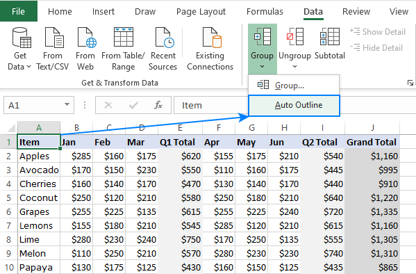
In our case, the Auto Outline feature created two groups for Q1 and Q2 data. If you also want an outer group for columns B — I, you’ll have to create it manually as explained in the first part of this tutorial. 
If your summary columns are placed to the left of the detail columns, proceed in this way:
- Click a small arrow in the lower-right corner of the Outline group, which is called the dialog box launcher.

In the Settings dialog box that pops up, clear the Summary columns to right of detail box, and click OK. 
After that, use the Auto Outline feature as explained above, and you will get the following result: 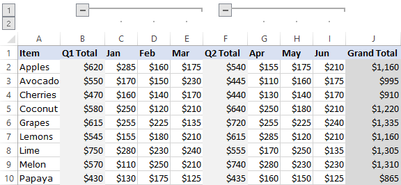
How to hide and show grouped columns
Depending on how many groups you want to cover up or display, use one of the below techniques.
Hide and show a particular column group
- To hide the data within a certain group, click the minus (-) sign for the group.
- To show the data within a certain group, click the plus (+) sign for the group.
Expand or collapse the whole outline to a given level
To hide or show the entire outline to a certain level, click the corresponding outline number.
For example, if your outline has three levels, you can hide all the groups of the second level by clicking the number 2. To expand all the groups, click the number 3.
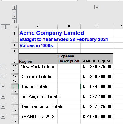
Hide and show all of the grouped data
- To hide all the groups, click the number 1. This will display the lowest level of detail.
- To display all the data, click the highest outline number. For example, if you have four levels, click the number 4.
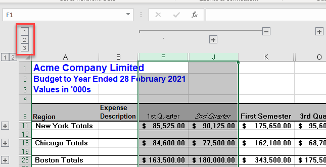
Our sample dataset has 3 outline levels:
Level 1 — only shows Items and Grand Total (columns A and J) while hiding all intermediate columns.
Level 2 – in addition to level 1, also displays Q1 and Q2 totals (columns E and I).
Level 3 — shows all the data. 
How to copy only visible columns
After hiding some column groups, you may want to copy the displayed data somewhere else. The problem is that highlighting the outlined data in the usual way selects all the data, including the hidden columns.
To select and copy only visible columns, this is what you need to do:
- Use the outline symbols to hide the columns that you don’t want copied.
- Select the visible columns using the mouse.
- On the Home tab, in the Editing group, click Find & Select >Go To.
- In the Go To Special dialog box, select Visible cells only, and click OK.
How to ungroup columns in Excel
Microsoft Excel provides an option to remove all groupings at once or ungroup certain columns only.
How to remove the entire outline
To remove all groupings at a time, go to the Data tab > Outline group, click the arrow under Ungroup, and then click Clear Outline. ![]()
- Clearing outline only removes the outline symbols; it does not delete any data.
- If some column groups were collapsed while clearing outline, those columns might remain hidden after the outline is removed. To display the data, undie columns manually.
- Once the outline is cleared, it’s not possible to get it back with Undo. You will have to recreate the outline from scratch.
How to ungroup specific columns
To remove grouping for certain columns without removing the entire outline, these are the steps to perform:
- Select the rows you want to ungroup. For this, you can hold down the Shift key while clicking the plus (+) or minus (-) button for the group.
- On the Data tab, in the Outline group, and click the Ungroup button. Or press the Shift + Alt + Left Arrow keys together, which is the ungrouping shortcut in Excel.
That’s how to group and auto outline columns in Excel. I thank you for reading and hope to see you on our blog next week.
Источник
Get a handle on your data
Grouping rows and columns in Excel lets you collapse and expand sections of a worksheet. This can make large and complex datasets much easier to understand. Views become compact and organized. This article shows you step-by-step how to group and view your data.
Instructions in this article apply to Excel 2019, 2016, 2013, 2010, 2007; Excel for Microsoft 365, Excel Online and Excel for Mac.
Grouping in Excel
You can create groups by either manually selecting the rows and columns to include, or you can get Excel to automatically detect groups of data. Groups can also be nested inside other groups to create a multi-level hierarchy. Once your data is grouped, you can individually expand and collapse groups, or you can expand and collapse all groups at a given level in the hierarchy.
Groups provide a really useful way to navigate and view large and complex spreadsheets. They make it much easier to focus on the data that’s important. If you need to make sense of complex data you should definitely be using Groups and could also benefit from Power Pivot For Excel.
How to Use Excel to Group Rows Manually
To make Excel group rows, the simplest method is to first select the rows you want to include, then make them into a group.
-
For the group of rows you want to group, select the first row number and drag down to the last row number to select all the rows in the group.
-
Select the Data tab > Group > Group Rows, or simply select Group, depending on which version of Excel you’re using.
-
A thin line will appear to the left of the row numbers, indicating the extent of the grouped rows.
Select the minus (-) to collapse the group. Small boxes containing the numbers one and two also appear at the top of this region, indicating the worksheet now has two levels in its hierarchy: the groups and the individual rows within the groups.
-
The rows have been grouped and can now be collapsed and expanded as required. This makes it much easier to focus on just the relevant data.
How to Manually Group Columns in Excel
To make Excel group columns, the steps are almost the same as doing so for rows.
-
For the group of columns you want to group, select the first column letter and drag right to the last column letter, thereby selecting all the columns in the group.
-
Select the Data tab > Group > Group Columns, or select Group, depending on which version of Excel you’re using.
-
A thin line will appear above the column letters. This line indicates the extent of the grouped columns.
Select the minus (-) to collapse the group. Small boxes containing the numbers one and two also appear at the top of this region, indicating the worksheet now has two levels in its hierarchy for columns, as well as for rows.
-
The rows have been grouped and can now be collapsed and expanded as required.
How to Make Excel Group Columns and Rows Automatically
While you could repeat the above steps to create each group in your document, Excel can automatically detect groups of data and do it for you. Excel creates groups where formulas reference a continuous range of cells. If your worksheet doesn’t contain any formulas, Excel won’t be able to automatically create groups.
Select the Data tab > Group > Auto Outline and Excel will create the groups for you. In this example, Excel correctly identified each of the groups of rows. Because there’s no annual total for each spending category, it has not automatically grouped the columns.
This option isn’t available in Excel Online, if you’re using Excel Online, you’ll need to create groups manually.
How to Create a Multi-Level Group Hierarchy in Excel
In the previous example, categories of income and expense were grouped together. It would make sense to also group all of the data for each year. You can do this manually by applying the same steps as you used to create the first level of groups.
-
Select all of the rows to be included.
-
Select the Data tab > Group > Group Rows, or select Group, depending on which version of Excel you are using.
-
Another thin line will appear to the left of the lines representing the existing groups and indicating the extent of the new group of rows. The new group encompasses two of the existing groups and there are now three small numbered boxes at the top of this region, signifying the worksheet now has three levels in its hierarchy.
-
The spreadsheet now contains two levels of groups, with individual rows within the groups.
How to Automatically Create Multi-Level Hierarchy
Excel uses formulas to detect multi-level groups, just as it uses them to detect individual groups. If a formula references more than one of the other formulas which define groups, this indicates these groups are part of a parent group.
Keeping with the cash flow example, if we add a Gross Profit row to each year, which is simply the income minus the expenses, then this allows Excel to detect that each year is a group and the income and expenses are sub-groups within these. Select the Data tab > Group > Auto Outline to automatically create these multi-level groups.
How to Expand and Collapse Groups
The purpose of creating these groups of rows and/or columns is that it allows regions of the spreadsheet to be hidden, providing a clear overview of the entire spreadsheet.
-
To collapse all of the rows, select the number 1 box at the top of the region to the left of the row numbers.
-
Select the number two box to expand the first level of groups and make the second level of groups visible. The individual rows within the second level groups remain hidden.
-
Select the number three box to expand the second level of groups so the individual rows within these groups also become visible.
It’s also possible to expand and collapse individual groups. To do so, select the Plus (+) or Minus (-) that appears to mark a group that’s either collapsed or expanded. In this way, groups at different levels in the hierarchy can be viewed as required.
Thanks for letting us know!
Get the Latest Tech News Delivered Every Day
Subscribe
How to Group Rows and Columns in Excel Step-By-Step
Working on complicated and extensive spreadsheets is so difficult – it’s bound to give you a headache 🥴
Luckily, Excel has grouping and outlining functions.
They make the data more readable and understandable by grouping it together. Not only that, but you can also create outlines and collapse rows to focus on a single section of data.
Using these functions can be challenging at first but worry not. We’re here to teach you just that.
If you want a free practice copy to try these functions, download our sample workbook here.
How to group rows in Excel
Before we begin, we need to be familiar with something 🧐
There are two primary ways to group rows in Excel. One, group rows automatically. And two, group rows manually.
Grouping rows automatically is much easier and faster. Especially when you have only one level of information, like this:

But sometimes Excel may group incorrect data when grouping automatically. That’s especially when you have different levels of information, like this:

In such a case, we group the data manually.
With that being said, let’s see how to group rows in Excel both automatically and manually below.
How to automatically group rows in Excel
Suppose we have the following data that we want to group.

To group this data automatically:
- Select any cell from the data set.

- Go to the Data Tab.

- Under the Outline group, select Auto Outline from the Group option.

- Choose the Rows option from the Group dialog box.
- The grouped data and outline appear automatically 😉

These small boxes on the left side with the minus sign are outline symbols. And they represent each level.
These boxes act like layers you can hide or show at any time to make your data more concise. It is similar to the tool used in Adobe Illustrator 🖼️
You can collapse a particular level by clicking its corresponding outline box. Like this:

And press the plus sign to expand the rows:

We also have the outline number of each group at the top.
1 always represents the least amount of data. This is the condition where the rows are collapsed. Like this:

Similarly, number 2 represents ungrouped data.

Make sure there are no hidden rows in the Excel sheet when you group data. Excel might perform the task incorrectly.
How to group rows manually in Excel
We saw earlier that Excel grouped rows automatically. But it didn’t include an outline of the whole data set. Using that outline, we would have been able to hide the entire data set.
So, how do we do that?
For that, we will group the rows manually 🔒
We will first remove the previous outline.
How to remove outlines
- Click Clear Outline from the Ungroup option under the Outline group.

- The outline disappears.

To manually group rows, we will first create the outermost outline. And then move toward the other levels.
To create the outermost outline:
- Select the whole data

- From the Data Tab, click Group under the Outline group.

- The outermost outline appears.

Collapsing this will hide the entire data set.
Now, for the other level, we will select a particular level each time and then group the rows together 😀
For instance, we will group the first level from A2:A4.
- Select the rows.

- Select the Group option from the Outline group.
- The selected rows have been grouped, and the outline appears.

- Perform the same steps with the remaining levels until the result looks like this.

As visible, there are three number boxes in the outline this time. Contrary to what we saw earlier in automatic Excel grouping, choosing the first box here will hide all the data.
The second box will show a part of the data, and the third box will show the entire data set.
How to group rows with the SUBTOTAL function
You can also subtotal rows in all the groups using the SUBTOTAL function. You can apply the COUNT, SUM, AVG, MIN, and MAX functions to your data.
Let’s understand this with the following example data.

- Click anywhere on the dataset and press the Subtotal button.

- The Dialog box appears.
Select the places you want to add subtotal to.

Put a checkmark on the ‘Summary below data’ option. It displays the result of the chosen function beneath the data. You can also change the function you want from the options.
The summary row looks like this:

The SUBTOTAL function automatically creates an outline along with the Grand total. Hence, you can use it to get two tasks done at the same time 🤓
And that’s it about grouping rows in Excel 🤗
How to group columns in Excel
Grouping columns in excel is the same as grouping rows. It is used when your data extends from left to right instead of top to bottom.
The only difference is that the outline appears on the top of the sheet instead of appearing on its left.
Let’s see how this works.
We will use the previous data set. And here, we want to group the columns.

We will first create the outermost outline and group all the data.

Now we will group each column individually, starting from column B – Mangoes.
- Select the column heading and click Group.
- Choose the Column option from the dialog box.
- Press Enter

- Repeat the same process with the remaining columns.

All your columns have now been grouped.
That’s it – Now what?
Knowing how to group rows or columns is very important. It helps organize data and improves the readability of complex and detailed information.
In this article, we learned how to group data in Excel and how to make a clear outline. These are some of the most useful features of Excel, but there’s so much more to learn.
If you are new to this giant spreadsheet software, we suggest you start by mastering the essential intermediate functions. These include VLOOKUP, IF, and SUMIF functions.
Join my 30-minute free email course to learn these fantastic functions and many more.
Other resources
The best part about grouping rows and columns in Excel is that it lets you focus on a small section of data instead of the whole sheet.
If you like this article, you might want to read some other articles like the SUBTOTAL function, FILTER function, or hiding rows. 😃
Frequently asked questions
To auto-outline data in Excel, select any cell from the data set. Go to the Data Tab. Select the Auto outline option under the Outline Group from the top right corner. From the dialog box, select the way you want to group your data and press Enter. Your data has been grouped.
You need to group the data manually to group rows by cell value. Divide your data into different levels. Select each level individually and group it using the Group option.
Kasper Langmann2022-12-13T00:00:36+00:00
Page load link
This tutorial will demonstrate how to Group Cells (Rows / Columns) in Excel & Google Sheets.
Grouping or outlining data in Excel allows us to hide or show rows or columns depending on how much detail we wish to see on the screen. Different levels can be displayed according to your needs. Excel allows up to 8 levels of grouping. To use the group function in Excel, the data really needs to be organized in your worksheet in a specific way that works with the grouping functionality.
Manually Grouping or Ungrouping Rows
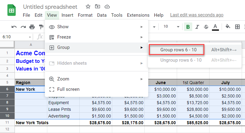
1. To group a number of rows together, first, highlight the rows you wish to group.
2. In the Ribbon, select Data > Outline > Group >Group.
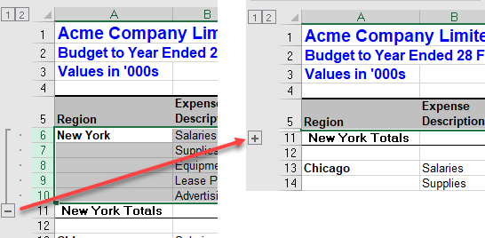
3. A small minus sign will be added into the outline bar on the left of the screen. Clicking on the minus sign allows us to collapse the group and the minus sign will then change to a plus sign indicating that there is hidden data within the outline.
4. We can repeat manual grouping to add more groups to the worksheet as required.
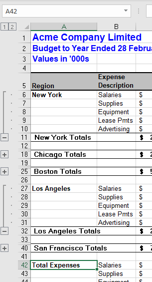
5. As well as using the plus and minus outline symbols, we can also use the 1 or 2 in the top left hand corner of the screen to expand or collapse all the groups.
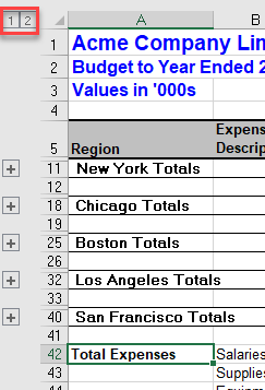
6. Clicking on the 1 will collapse all the groups while clicking on 2 will expand all the groups.
Manually Grouping or Ungrouping Columns
1. To group a number of columns together, first, highlight the columns you wish to group. This can be done if you have rows already grouped or not.
2. In the Ribbon, select Data > Outline > Group >Group to group the columns together. Repeat this until you have created all the groups that you require.
3. Once we have grouped our rows and / or columns, we can add a new level but grouping once again. This will add a third level of grouping to the outline symbols in the top left hand corner of the screen.
4. Once again, we can repeat this across our worksheet, and add up to 8 levels of grouping.
Ungrouping Rows or Columns
1. Highlight the group you wish to ungroup and then, in the Ribbon, select Data > Outline > Ungroup > Ungroup.
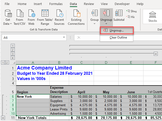
This will only remove the one group.
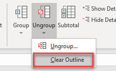
2. To remove all the grouping in the worksheet, click anywhere in the data and then, in the Ribbon, select Data > Outline > Ungroup > Clear Outline.
Auto-Outline
We can use the Auto Outline function of Excel as long as our data is logically organized so that Excel recognizes the groups within the rows and columns. There must not be any blank rows in the data and the data must be summed or subtotaled at each level.
1. Click anywhere in the data where you wish the outline to be created and then, in the Ribbon, select Data > Outline > Group > Auto Outline.
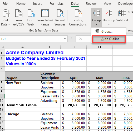
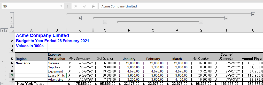
2. Excel will create as many grouping levels as the logical layout of the data allows.
How to Group Cells in Google Sheets
Google Sheets only allows us to manually group or ungroups rows and columns of data.
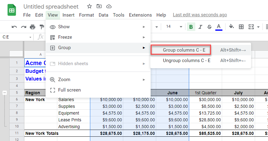
1. Select the rows you wish to group and then, in the Menu, select View > Group > Group rows (the number of rows selected will be shown).
2. Similarly, select the columns you wish to group and then in the Menu, select View > Group > Group columns (the number of columns selected will be shown).
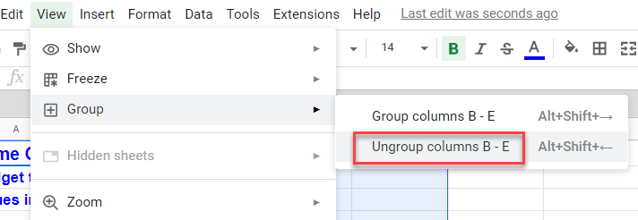
3. To ungroup rows or columns, click in the group you wish to ungroup and then in the Menu, select View > Group > Ungroup (rows or columns).
The best way to keep spreadsheets organized
Guide on How to Group in Excel
Grouping rows and columns in Excel[1] is critical for building and maintaining a well-organized and well-structured financial model. Using the Excel group function is the best practice when it comes to staying organized, as you should never hide cells in Excel. This guide will show you how to group in Excel with step-by-step instructions, examples, and screenshots.
Keyboard Shortcuts Sheet
Looking to be an Excel wizard? Increase your productivity with CFI’s comprehensive keyboard shortcuts guide.
Excel Group Function
The Excel group function is one of the best secrets a world-class financial analyst uses to make their work extremely organized and easy for other users of the spreadsheet to understand.
Reasons to use the Excel Group Function:
- To easily expand and contract sections of a worksheet
- To minimize schedules or side calculations that other users might not need
- To keep information organized
- As a substitute for creating new sheets (tabs)
- As a superior alternative to hiding cells
The function is found in the Data section of the Ribbon, then Group.
Example of How to Group in Excel
Let’s look at a simple exercise to see how it works. Suppose we have a schedule in a worksheet that is becoming quite long, and we want to reduce the amount of detail that’s shown. The screenshots below will show you how to properly implement grouping in Excel.
Here are the steps to follow to group rows:
- Select the rows you wish to add grouping to (entire rows, not just individual cells)
- Go to the Data Ribbon
- Select Group
- Select Group again
You can repeat the steps above as many times as you like, and you can also apply it to columns as well.
Once you’re finished, you can press the “-” buttons in the margin to collapse the rows or columns.
If you want to expand them again, press the “+” buttons in the margin, as shown in the screenshot below.
There is also a “1” button in the top left corner to collapse all groups, and a “2” button to expand all groups.
Why You Should Never Hide Cells in Excel
Though many people do it, you should never hide cells in Excel (or spreadsheets either, for that matter). The reason is that Excel does not make it clear to the user of the spreadsheet that cells have been hidden, and thus they may go unnoticed.
The only way to see that cells are hidden is to notice that the row number or column number suddenly jumps (e.g., from row 25 to row 167).
Since other users of the spreadsheet may not notice this (and you may forget yourself) you should never hide cells in Excel.
Download Excel Group Template
You can download the Template for free if you wish to use it as an example or starting point for how to group in Excel and apply it to your own work and financial analysis.
Additional Resources
Thank you for reading CFI’s guide to Group in Excel. To continue learning and advancing your career, these additional CFI resources will be helpful:
- List of 300+ Excel Functions
- Keyboard Shortcuts
- What is Financial Modeling?
- Financial Modeling Courses
- See all Excel resources