Column formatting in excel - Word и Excel - помощь в работе с программами

Excel provides numerous predefined table styles that you can use to quickly format a table. If the predefined table styles don’t meet your needs, you can create and apply a custom table style. Although you can delete only custom table styles, you can remove any predefined table style so that it is no longer applied to a table.

You can further adjust the table formatting by choosing Quick Styles options for table elements, such as Header and Total Rows, First and Last Columns, Banded Rows and Columns, as well as Auto Filtering.

Note: The screen shots in this article were taken in Excel 2016. If you have a different version your view might be slightly different, but unless otherwise noted, the functionality is the same.

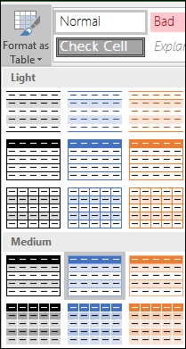
Choose a table style

When you have a data range that is not formatted as a table, Excel will automatically convert it to a table when you select a table style. You can also change the format for an existing table by selecting a different format.

Select any cell within the table, or range of cells you want to format as a table.
On the Home tab, click Format as Table.
Click the table style that you want to use.

Notes:

Auto Preview — Excel will automatically format your data range or table with a preview of any style you select, but will only apply that style if you press Enter or click with the mouse to confirm it. You can scroll through the table formats with the mouse or your keyboard’s arrow keys.
When you use Format as Table, Excel automatically converts your data range to a table. If you don’t want to work with your data in a table, you can convert the table back to a regular range while keeping the table style formatting that you applied. For more information, see Convert an Excel table to a range of data.

Important:

Once created, custom table styles are available from the Table Styles gallery under the Custom section.
Custom table styles are only stored in the current workbook, and are not available in other workbooks.

Create a custom table style

Select any cell in the table you want to use to create a custom style.
On the Home tab, click Format as Table, or expand the Table Styles gallery from the Table Tools > Design tab (the Table tab on a Mac).
Click New Table Style, which will launch the New Table Style dialog.
In the Name box, type a name for the new table style.
In the Table Element box, do one of the following:
- To format an element, click the element, then click Format, and then select the formatting options you want from the Font, Border or Fill tabs.
- To remove existing formatting from an element, click the element, and then click Clear.
Under Preview, you can see how the formatting changes that you made affect the table.
To use the new table style as the default table style in the current workbook, select the Set as default table style for this document check box.

Delete a custom table style

Select any cell in the table from which you want to delete the custom table style.
On the Home tab, click Format as Table, or expand the Table Styles gallery from the Table Tools > Design tab (the Table tab on a Mac).
Under Custom, right-click the table style that you want to delete, and then click Delete on the shortcut menu.

Note: All tables in the current workbook that are using that table style will be displayed in the default table format.

Select any cell in the table from which you want to remove the current table style.
On the Home tab, click Format as Table, or expand the Table Styles gallery from the Table Tools > Design tab (the Table tab on a Mac).
Click Clear.

The table will be displayed in the default table format.

Note: Removing a table style does not remove the table. If you don’t want to work with your data in a table, you can convert the table to a regular range. For more information, see Convert an Excel table to a range of data.

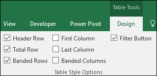
There are several table style options that can be toggled on and off. To apply any of these options:

Select any cell in the table.
Go to Table Tools > Design, or the Table tab on a Mac, and in the Table Style Options group, check or uncheck any of the following:
- Header Row — Apply or remove formatting from the first row in the table.
- Total Row — Quickly add SUBTOTAL functions like SUM, AVERAGE, COUNT, MIN/MAX to your table from a drop-down selection. SUBTOTAL functions allow you to include or ignore hidden rows in calculations.
- First Column — Apply or remove formatting from the first column in the table.
- Last Column — Apply or remove formatting from the last column in the table.
- Banded Rows — Display odd and even rows with alternating shading for ease of reading.
- Banded Columns — Display odd and even columns with alternating shading for ease of reading.
- Filter Button — Toggle AutoFilter on and off.

In Excel for the web, you can apply table style options to format the table elements.

Choose table style options to format the table elements

There are several table style options that can be toggled on and off. To apply any of these options:

Select any cell in the table.
On the Table Design tab, under Style Options, check or uncheck any of the following:
- Header Row — Apply or remove formatting from the first row in the table.
- Total Row — Quickly add SUBTOTAL functions like SUM, AVERAGE, COUNT, MIN/MAX to your table from a drop-down selection. SUBTOTAL functions allow you to include or ignore hidden rows in calculations.
- Banded Rows — Display odd and even rows with alternating shading for ease of reading.
- First Column — Apply or remove formatting from the first column in the table.
- Last Column — Apply or remove formatting from the last column in the table.
- Banded Columns — Display odd and even columns with alternating shading for ease of reading.
- Filter Button — Toggle AutoFilter on and off.

Источник

Application examples of formatting Excel data of various types for computationally intensive calculations.

Changing of cells format in data tables

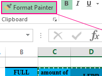Format Painter in Excel for table layout.
Multiple copies of table cell formats on multiple sheets using the Format Painter tool. Copying the width of columns and rows of a sheet.

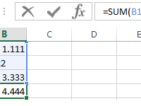Influence of the cell format on working of the SUM function.
The possible errors in the summation, where there is a comma instead of a dot. Quick search of incorrect fractional numbers. Automatic assignment of the cell formats with the SUMM function.

Transfer of data from one Excel table to another one.
You can transfer table data within one sheet, as well as to another sheet or to another file. In this case, you can copy either the entire table, or its individual values, properties or parameters.

Источник

The maximum width for a column is 255 if the default font and font size is used. The minimum width is zero, of course. If a column width is zero, the column will be hidden.

To set a column to a specific width, select the column that you want to format.

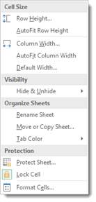
Next, go to the Cells group under the Home tab. Click the Format dropdown menu.

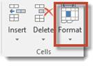
Pictured below is the dropdown menu.

Select Column Width.

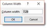
Type in the width of the column, keeping in mind that it reflects the number of characters that can be displayed.

Change the Width of the Column to Fit the Contents

Maybe you just want to make sure that the columns are wide enough to display all the contents, but you don’t want to take the time to count characters. Perhaps you aren’t even sure how many characters there will be, but want to make sure the column will be wide enough anyway.

To do this, go back to the Format dropdown menu. This time select AutoFit Column Width.

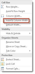
The width of all the cells in a selected column will now be determined by the cell with the most characters.

Match the Column Width to Another Column’s Width

You can also match the width of one column to the width of another column. To do this, select the column whose width you want to match.

Copy the column by right clicking and selecting copy.

Next, select the column whose width you want to change. Right click within a cell in that column and select Paste Special.

Put a check by Column Widths, then click OK.

As you can see, the column width of column D has been expanded to match the column width in column B.

Change the Default Width for All Columns in a Worksheet or Workbook

To change a default column width for a worksheet, click the worksheet tab to make the worksheet active. To change it for the entire workbook, click a worksheet tab, then right click, and select Select All Sheets.

Now, go back to the Home tab and click the Format dropdown arrow again.

Select Default Width.

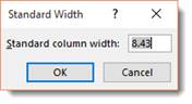
In the Standard Width box, type the new measurement.

Change the Width of Columns by Moving the Mouse

To change the width of one column using your mouse, drag the right side of the column to the right until you reach the desired width. To do so, move your mouse to the line separating two columns until you see horizontal arrows appear.

To change the width of multiple columns, select the columns that you want to change, then drag the right side of one column to its desired width.

To change the width of all the columns in a worksheet, select the entire worksheet by clicking the box to the left of column A and above row 1, then dragging the boundary of any column.

Changing Rows to a Specific Height

You follow the exact same steps to change row height as you did for columns.

To change a row to a specific height, select the row(s) that you want to change.

Go to the Home tab and click the dropdown arrow below Format.

Select Row Height.

Row height is measured in points. In the snapshot above, the row height is set at 15 points. This is the same size as font size 15.

Enter the row height, then click OK.

Change Row Height to Fit Contents

Just as you changed the width of a column to fit the contents of the widest cell in a column, you can also change the height of a row to match the height of the tallest cell.

To do this, select the rows(s) that you want to change.

Select AutoFit Row Height from the Format dropdown menu on the Ribbon.

Change a Row Height by Dragging the Mouse

You can also change the height of a row(s) by simply dragging the mouse.

To do this, select the row(s) whose height you want to change.

Next, drag the boundary below a row to adjust its height. To adjust the height of multiple rows, drag the boundary of one of them.

Источник

Definition of Format Cells

A format in excel can be defined as the change of appearance of the data in the cell the way it is, without changing the actual data or numbers in the cells. That means the data in the cell remains the same, but we will change the way it looks.

Different Formats in Excel

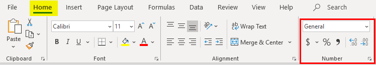
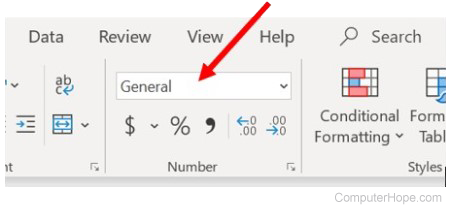
We have multiple formats in Excel to use. To see the available formats in excel, click on the “Home” menu on the top left corner.

General Format

In General format, there is no specific format; whatever you input, it will appear in the same way; it may be a number or text or symbol. After clicking on the HOME menu, go to the “NUMBER” segment, where you can find a drop of formats.

Click on the drop-down where you see the “General” option.

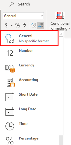
We will discuss each of these formats one by one with related examples.

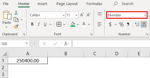
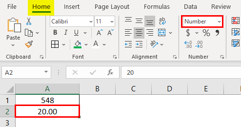
1. Number Format

This format converts the data to a number format. When we input the data initially, it will be in General format; after converting to Number format only, it will appear as number format. Observe the below screenshot for the number in General format.

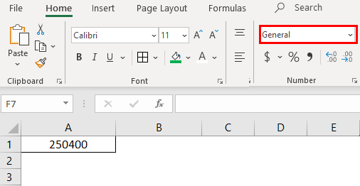
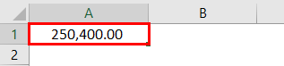
Now choose the format “Number” from the drop-down list and see how the appearance of cell A1 changes.

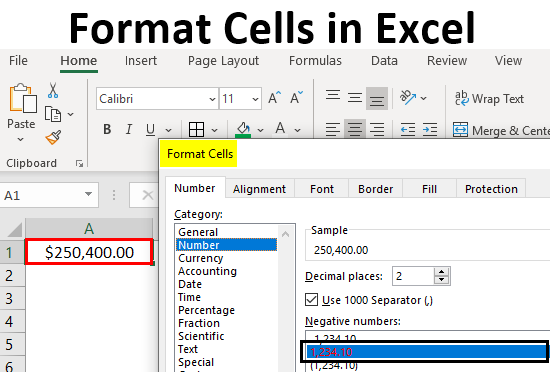
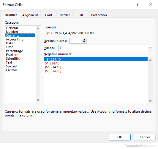
That is a difference between the General and Number format. If you want further customizations to your number format, select the cell that you want to do customization and right-click the below menu will come.

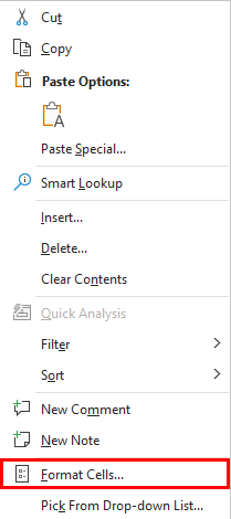
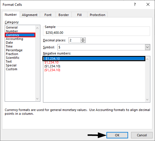
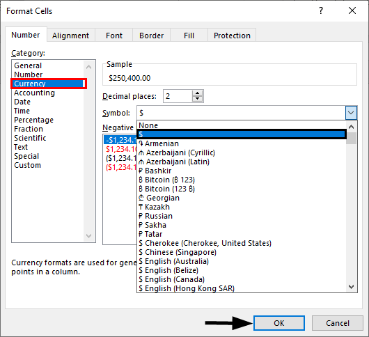
Choose the “Format Cells“ option then you will get the below window.

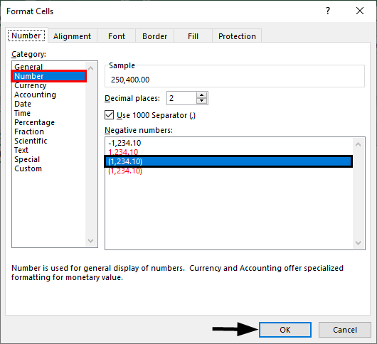
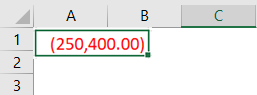
Choose “Number” under the “Category” option then you will get the customizations for the Number format. Choose the number of decimals you want to display. Tick the checkbox “Use 1000 separator” for separation of 1000’s with a comma (,).

Choose the negative number format whether you want to display with a negative symbol, brackets, red colour, nd red col, etc.

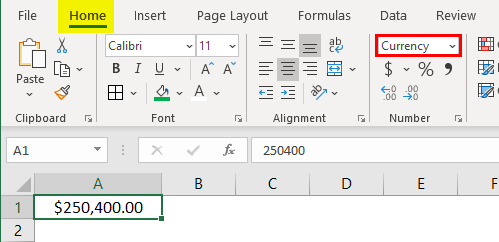
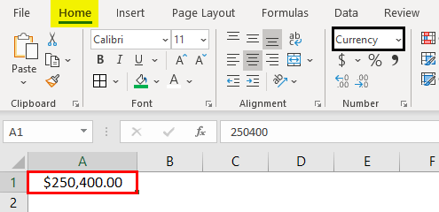
2. Currency Format

Currency format helps to convert the data to a currency format. We have an option to choose the type of currency as per our requirement. Select the cell which you want to convert to Currency format and choose the “Currency” option from the drop-down.

Currently, it is in Dollar currency. We can change by clicking on the drop-down of “$” and choose your required currency.

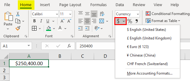
In the drop-down, we have few currencies; if you want the other currencies, click on the option “More Accounting formats”, which will display a pop-up menu as below.

Click on the drop-down “Symbol” and choose the required currency format.

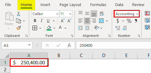
3. Accounting Format

As you all know, accounting numbers are all related to money; hence whenever we convert any number to accounting format, it will add a currency symbol to that. The difference between currency and accounting is currency symbol alignment. Below are the screenshots for reference.

4. Accounting Alignment

5. Currency Alignment

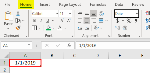
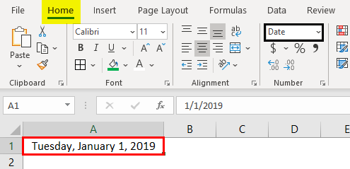
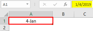
6. Short Date Format

A date can represent in a short format and long format. When you want to represent your date in a short format, use the short date format. E.g., 1/1/2019.

7. Long Date Format

The long date is used to represent our date in an expandable format like the below screenshot.

We see the short date format and long date format have multiple formats to represent our dates. Right-click and select “Format Cells” as to how we did before for “numbers”, then we will get the window to select the required formats.

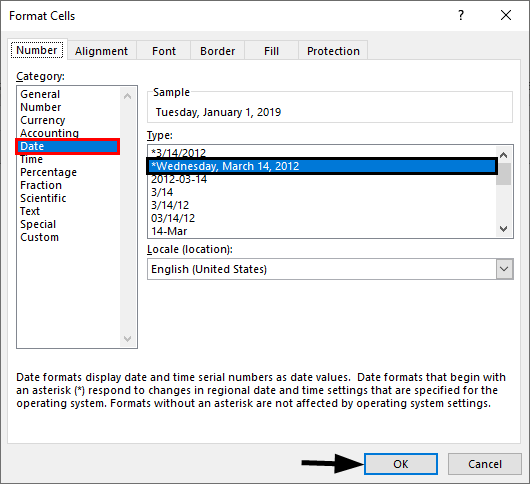
You can choose the location from the “Locale” drop-down menu.

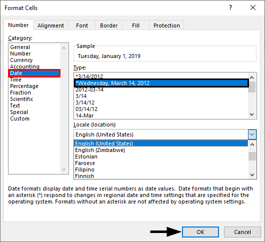
Choose the date format under the “Type” menu.

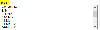
We can represent our date in any of the formats from the available formats.

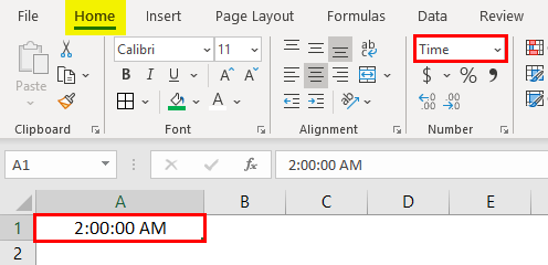
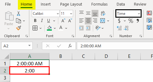
8. Time Format

This format is used to represent the time. If you input time without converting the cell into time format, it will show normally, but if you convert the cell into time format and input, it will clearly represent the time. Find the below screenshot for the differences.

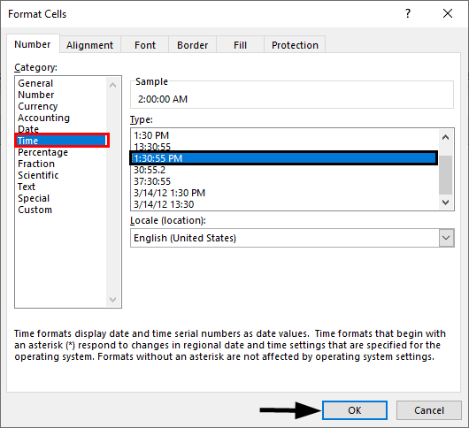
If you still want to change the time format, then change in the format cells menu as shown below.

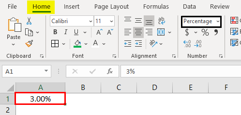
9. Percentage Format

Suppose you want to represent the number percentage use this format. Input any number in the cell and select that cell and choose the percentage format then the number will convert into a percentage.

10. Fraction Format

When we input the fraction numbers like 1/5, we should convert the cells into Fraction format. If we input the same 1/5 in a normal cell, it will show as a date.

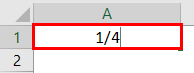
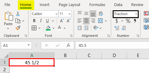
This is how the fraction format works.

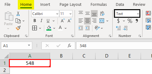
11. Text Format

When you input the number and convert it to text format, the number will align to the left side. It will consider as text as only, not the number.

12. Scientific Format

When you input a number 10000 (Ten thousand) and convert it into a scientific format, it will display as 1E+04, here E means exponent and 04 represents the number of zeros. If we input the number 0.0003, it will display as 3E-04. Try different numbers in excel format and check you will get a better idea to understand this better.

13. Other Formats

Apart from the explained formats, we have other formats like Alignment, Font, Border, Fill, and Protection.

Most of them are self-explanatory; hence I am leaving and explaining protection alone. When you want to lock any cells in the spreadsheet, use this option. But this lock will enable only when you protect the sheet.

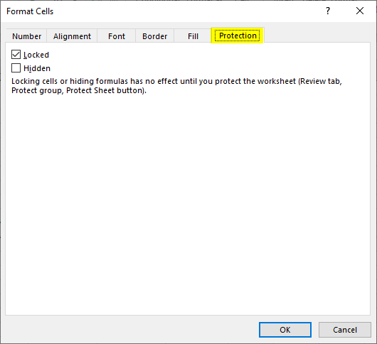
You can hide and lock the cells on the same screen; Excel has provided instructions on when it will affect.

Things to Remember About Format Cells in Excel

One can apply formats by right-clicking and selecting the format cells or from the drop-down as explained initially. The impact of them is the same; however, you will have multiple options when you right-click.
When you want to apply a format to another cell, use format painter, select the cell, click on formatted painters, and choose the cell you want to apply.
Use the option “Custom” when you want to create your own formats as per requirement.

Change font type, size, or color of data in a cell

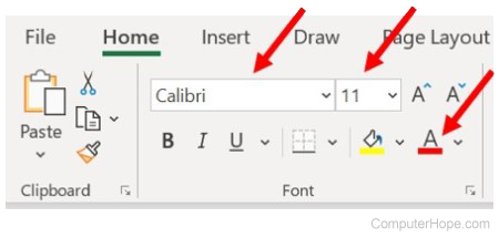
To change the font type, size, or color, select the cell you want to change, then the appropriate option on the Home tab Font section on the Ribbon.

How to select one or more cells in a spreadsheet program.
How to change the font color, size, or type in Excel.

Set data to be bold, italic, or underlined in a cell

In Excel, you can set data in a cell to be bold, italic, or underlined, to help bring attention to it.

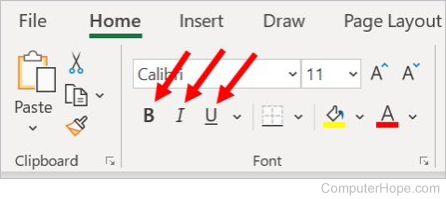
To change a cell’s text format, on the Home tab Font section of the Ribbon, click the B icon for bold, I icon for italic, or U icon for underline.

Change the background color of a cell

In Excel, you can change the background color of a cell to a wide variety of colors to highlight specific data in a spreadsheet.

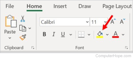
To fill in the background color of a cell, select the cell you want to change. On the Home tab Font section on the Ribbon, click the paint bucket. Select the desired background color from the drop-down window, or click More Colors.

Add a border around one or more cells

In Excel, you can add a border around one or more cells, to group or separate them, improving both visibility and readability of data. You can also choose from different types of borders, and customize their thickness.

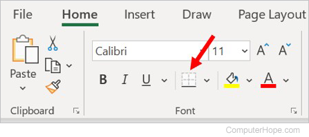
To set a border around cells, select the cells that you want to add a border. On the Home tab Font section on the Ribbon, click the icon with a cross and black line on the bottom of the box. In the drop-down window, select the type of border you want to add around the cells.

For additional border styles and options, right-click the selected cells and choose Format Cells. Click the Border tab in the Format Cells window, and select the style of border you prefer.

Change the alignment of data in a cell

In Excel, you can change the horizontal and vertical alignment of data in a cell. You can also indent the data in a cell, if desired.

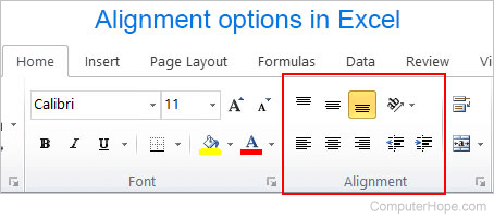
To change the alignment or indentation, select the cell you want to change. On the Home tab, in the Alignment section on the Ribbon, click the desired alignment option icon. The horizontal alignment options have 3 lines in the icon (top row of icons) and the vertical alignment options have 6 lines in the icon (bottom row of icons).

To indent data in a cell, click the icon with two bold lines and an arrow pointing to the right. To remove indentation of data in a cell, click the icon with two bold lines and an arrow pointing to the left.

How to align text in Microsoft Excel, Calc, and Google Sheets.

Change the data type for a cell

In Excel, you can change, or format, the type of data in a cell. For example, you can change the data to display a currency, displaying a currency symbol next to the left of it. Other data types you can change data to include numerical with decimal places, date, time, percentage, fraction, and text.

Select the cell that you want to change the data type. On the Home tab, Number section in the Ribbon, click the data type drop-down list, and select the data type.

If you want to change the data type to currency or percentage, click the dollar sign icon or the percent icon below the data type drop-down list. If you click the down arrow to the right of the dollar sign icon, you can choose between several currency types, including European and Chinese currencies.

In addition to the above method, you can change the cells format by following the steps below.

Right-click the cell.
Click Format cells.
In the Format Cells window (shown below), select the number format you’d like to use. For example, if you wanted the cell to be shown as a dollar amount, select Currency.

Format cells categories

Below is a brief description about each of the number format categories found in the Format Cells window.

General — Default format with no specific number format.
Number — General display for number with the ability of adjusting the decimal place.
Currency — Currency format for showing monetary values with the ability to adjust the decimal and symbol.
Accounting — Like the currency format with lining up the currency symbols and decimal points.
Date — Show the number in a date format. For example, 10/28/22 or October, 28, 2022.
Time — Show the number in a time format. For example, 6:01:20 PM.
Percentage — Show the number in a percentage format with the ability to adjust the decimal place.
Fraction — Display the number in a fraction format.
Scientific — Show the number in a scientific format, for example, 1.38E+19 with the ability to adjust decimal places.
Text — Treat any text in the cells only as text, even if it contains numbers.
Special — Special formatting for numbers including zip codes, phone number, and social security numbers.
Custom — Display numbers in one of several custom formats.

Set up conditional formatting for one or more cells

In Excel, you can set conditional formatting for a cell, based on data in that cell. Conditional formatting is useful for automatically setting a background color in a cell. A common use of conditional formatting is setting the background color to green, yellow, or red based on the numerical data in the cells.

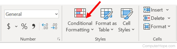
Select the cells where conditional formatting needs to be set. On the Home tab, in the Styles section on the Ribbon, click the Conditional Formatting icon and select a pre-defined rule or click New Rule to create your own.

If you selected a pre-defined conditional formatting rule, enter and select the applicable conditions and options in the window that opens. If you chose to create a new rule, select a Rule Type, then enter and select the applicable conditions and options in the New Formatting Rule window.

See our conditional formatting page for more information and help on setting up conditional formatting in your spreadsheet.

Change width of a column or height of a row

In Excel, the width of a column or the height of a row can be adjusted to fit all text or data. Making these width or height adjustments can make data in the spreadsheet easier to read and understand.

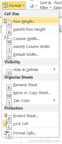
There are two ways you can change the width of a column or height of a row. On the Home tab, in the Cells section on the Ribbon, click the Format option. In the drop-down menu, select Column Width or Row Height to change the size of the selected column or row. In the Column Width or Row Height window that opens, enter the desired width or height value.

The second way is to use your mouse to change the column width or row height. For a column width change, in the horizontal header bar, place the mouse cursor between the column you want to change. The cursor changes to a cross with arrows on either side of the horizontal line in it. Press and hold the left mouse button, then drag the mouse to the left or right to change the column width. Release the left mouse button to set the new column width.

For a row height change, in the vertical header bar, place the mouse cursor between the row you want to change. The cursor changes to a cross, with arrows on top and bottom of the vertical line in the cross. Press and hold the left mouse button, then drag the mouse up or down to change the row height. Release the left mouse button to set the new row height.

Adjust the width and height of a spreadsheet column or row.

In Excel, the column headers are labeled as A, B, C, D, etc. Unfortunately, there is no ability to change these column headers. Instead, you need to enter names into row 1.

To set your own column headers, if you have data in row 1 of the spreadsheet, insert a new row above row 1. To make the column headers stand out from the rest of the data in the columns, consider adding background color and bold formatting.

How to add or remove a cell, column, or row in Excel.
How to change the name of the column headers in Excel.

Источник

This tutorial demonstrates how to apply conditional formatting rules to entire columns in Excel and Google Sheets.

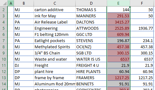
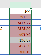
Apply Conditional Formatting to Entire Column

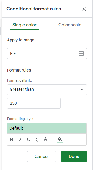
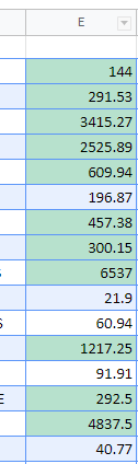
You can emphasize larger numbers in a dataset by highlighting all the cells in a column (e.g., E) that are greater than a specified value (e.g., 250) with a Conditional Formatting Rule.

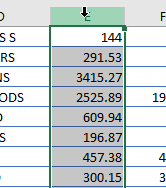
Click on the column header to select the entire column.

In the Ribbon, select Home > Conditional Formatting > Highlight Cells Rules > Greater Than…

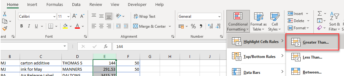
Type in the value you wish to test for, then select the format you require.

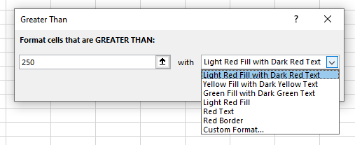
Click OK to apply the rule to the entire column.

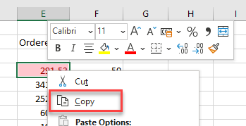
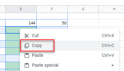
Copy Conditional Formatting From One Cell

Copy-Paste

If you already have a conditional formatting rule set for a specific cell, you can copy this format to the entire column with Paste Special.

Select the cell that has a conditional formatting rule and then right-click and click Copy (or use the keyboard shortcut CTRL + C).

Click on the column header of the required column and then right-click and click Paste Special > Paste Format.

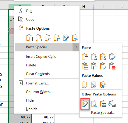
The conditional formatting rule that was applied to the original cell will now be applied to the entire column.

Format Painter

You can also copy the format applied to a single cell (in this case, conditional formatting) with the Format Painter feature.

Select the cell that has a conditional formatting rule and then, in the Ribbon, select Home > Clipboard > Format Painter.

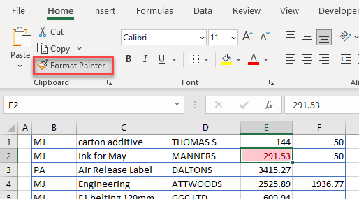
Click on the header of the column where you want the rule applied.

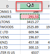
The conditional formatting rule that was applied to the original cell is applied to the entire column.

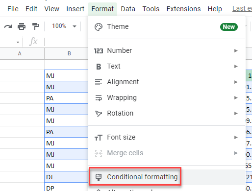
Apply to Entire Column in Google Sheets

You can also apply Conditional Formatting to an entire column in Google Sheets.

Apply Conditional Formatting

In the Menu, select Format > Conditional Formatting.

Click on the small square in the right of the Apply to range box.

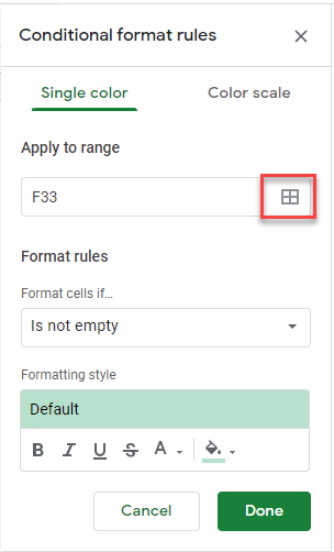
Select the column header of the column you wish to apply the conditional formatting rule to, then click OK.

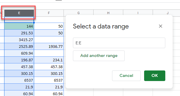
Create the rule in the Format cells if drop down box, and select the formatting style, and then click Done.

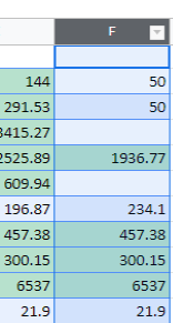
The rule is applied to the entire column.

Copy From One Cell

Copy-Paste

If you already have a cell or column with a Conditional Formatting rule set up, you can use Copy-Paste to copy the rule to another column.

Right-click on a cell that has the conditional formatting rule applied to it and click Copy (or use the keyboard shortcut CTRL + C).

Right click on the column header of the column you wish to apply the rule to, and then select Paste special > Format only (or use the keyboard shortcut CTRL + ALT + V).

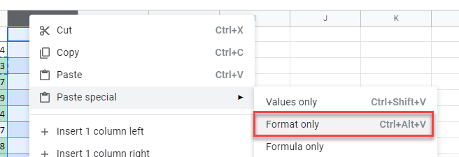
The conditional formatting rule is applied to the entire column you selected.

Paint Format

If you already have a cell or column with a conditional formatting rule set up, you can use Paint Format to copy the rule to another column.

Select the cell which has the conditional formatting rule applied.
In the Menu, select Paint format.

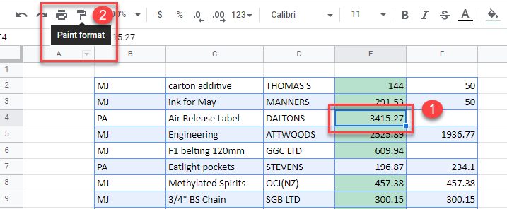
Click on the header of the column you wish to apply the rule to copy the conditional formatting to that column.

Источник

We’ve learned how to navigate Excel spreadsheets, resize rows and columns, and format numbers. But how do Excel experts get their sheets to look so beautiful? To answer that question, we’ll take a look at the options that Excel includes for cell formatting.

Basic text formatting

If we select any cell and head to the Home tab on the Ribbon, we’ll see some basic formatting options at the top of the ribbon: font style and size; bold, underline, and italics; and borders:

Of particular note are the font color and cell background color drop-downs, which allow us to style cells as we see fit:

To the right, we’ll see a number of paragraph options, including cell vertical alignment (top, middle, or bottom); horizontal alignment (left, right, and center); and indentation:

The «wrap text» option on this page allows us to toggle text wrapping within a cell on or off. If toggled on, text within a cell will automatically wrap to multiple lines rather than being cut off or just appearing on one line:

And, the «merge and center» button on this same tab allows us to merge multiple cells together to create headers. Try selecting a block of cells and hitting the «Merge» button to transform it into one larger block. We usually use this option at the top of charts, like so:

Advanced formatting

Looking for more cell formatting options? Try right-clicking a cell or selected range of cells; then hitting the Format Cells… button:

A cell formatting dialogue will appear with a number of tabs that allow us to format our spreadsheet in a ton of different ways:

The Number tab allows us to change number formats with some more expansive options, like commas (,) and number of decimal places.
The Alignment tab allows us to choose vertical and horizontal alignment; angle text; wrap text; and merge and center cells.
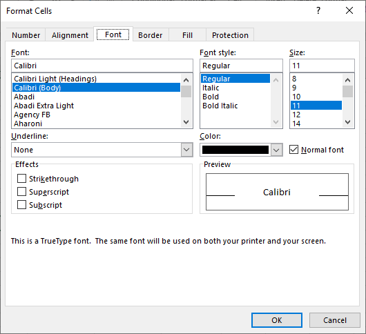
The Font tab allows us to modify text with features like colors; font styles; underlines; bold; italic; superscript; subscripts; strikethroughs; and different sizes.
The Border tab allows us to add various borders to our cells, including double borders, thick borders, and colored borders.
The Fill tab allows us to fill the backgrounds of cells with custom colors or patterns.

Take some time to explore the Format Cells dialogue to get a feel for all of the formatting options we have at our fingertips. We can combine these formatting options to beautify our spreadsheets in many different ways — so have fun and experiment to get a sense for what works well for you!

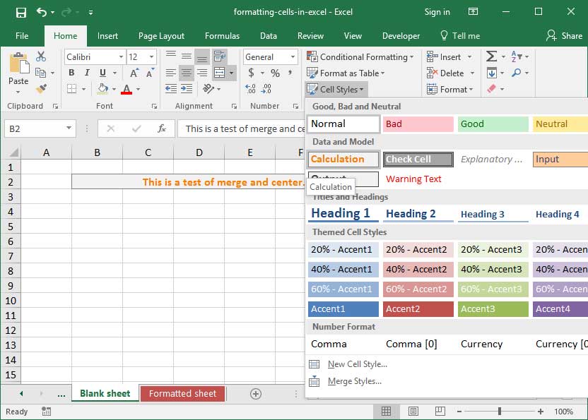
Custom styles

Excel also has a number of built-in Excel styles available for easy access. Check out the Cell Styles menu on the Home section of the ribbon to take a look at them. Using these preset styles is a great way to format our sheets with minimal effort while maintaining consistency across workbooks.

How we format our spreadsheets

Take a look at the below spreadsheet, which we’ve formatted using our standard procedure. Of course, formatting is totally subjective — so you can make your spreadsheet look however you want it to look — but consider the following as inspiration for where you might want to start.

In the above sheet, we’ve:

Formatted column headings with bold styling and a light blue cell background for easy viewing. We’ve also added a thick white border to the cells to differentiate them from each other.
Used Merge and Center on top of column headings, where appropriate.
Used appropriate number formats to accurately represent the quantities we’re analyzing.
Indented titles appropriately in the first column of our data set to represent the various components of different quantities. For example, Units sold and Sale price per unit are both components of Revenue, so they’re indented below it to represent dependency.
Used preset Cell Styles to represent key assumptions and outputs on our sheet.

Explore the 5 must-learn ‘fundamentals’ of Excel

Getting started with Excel is easy. Sign up for our 5-day mini-course to receive easy-to-follow lessons on using basic spreadsheets.

The basics of rows, columns, and cells…
How to sort and filter data like a pro…
Plus, we’ll reveal why formulas and cell references are so important and how to use them…

Comments

Источник

Formatting in Excel (2016, 2013 & 2010 and Others)

Formatting in Excel is a neat trick used to change the appearance of the data represented in the worksheet. We can do formatting in multiple ways, such as we can format the font of the cells or format the table by using the “Styles” and “Format” tabs available in the “Home” tab.

Formatting in Excel (2016, 2013 & 2010 and Others)
- How to Format Data in Excel? (Step by Step)
- Shortcut Keys to Format Data in Excel
- Things to Remember
- Recommended Articles

How to Format Data in Excel? (Step by Step)

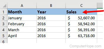
Let us understand the working of data formatting in Excel by simple examples. Now, suppose we have a simple report of sales for an organization as below:

You can download this Formatting Excel Template here – Formatting Excel Template

This report is not attractive to viewers. Therefore, we need to format the data.

Now, to format data in Excel, we must do the following:

Bold the text of the column header.
Make the font size larger.
Adjust the column width using the shortcut key (Alt+H+O+I) after selecting the whole table (Ctrl+A).
Align the data in the center.
Apply the outline border by using (Alt+H+B+T)
Apply background color using the “Fill Color” command available in the “Font” group on the “Home” tab

We will be applying the same format for the table’s last “Total” row by using the “Format Painter” command available in the “Clipboard” group on the “Home” tab.

As the amount collected is a currency, we should format the same as “Currency” using the command available in the “Number” group placed on the “Home” tab.

After selecting the cells we need to format as currency, we need to open the “Format Cells” dialog box by clicking the above arrow.

Choose “Currency” and click on “OK.“

We can also apply the outline border to the table.

We will be creating the label for the report by using “Shapes.” To make the shape above the table, we need to add two new rows. So, we will select the row by “Shift+Spacebar” and then insert two rows by pressing “Ctrl+’+” twice.

We must choose an appropriate shape from the “Shapes” command available in the “Illustration” group in the “Insert” tab to insert the shape.

Create the shape according to the requirement and with the same color as the heads of the column. Then, add the text on the shape by right-clicking on the shapes and choosing “Edit Text.”

We can also use the “Format” contextual tab for formatting the shape using various commands such as “Shape Outline,” “Shape Fill,” “Text Fill,” “Text Outline,” etc. We can also apply the excel formatting on textText formatting in Excel include changing the colour, font name, font size, alignment, font appearance in bold, underlining, italic, background colour of the font cell, and so on.read more using the commands available in the “Font” group placed on the “Home” tab.

We can also use “Conditional Formatting” to take the viewers’ attention to the “Top 3” salesperson and “Bottom 3” salesperson.

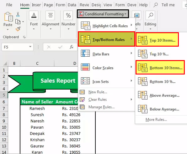
Format the cells that rank in the “Top 3” with “Green Fill with Dark Green Text.”

Also, format the cells that rank in the “Bottom 3” with “Light Red with Dark Red Text.”

We can also apply another conditional formatting option, “Data Bars.”

We can also create a chart to display the data, part of “Data Formatting Excel.”

Shortcut Keys to Format Data in Excel

To make the text bold: Ctrl+B or Ctrl+2
To make the text italic: Ctrl+I or Ctrl+3
To make the text underline: Ctrl+U or Ctrl+4
To make the font size of the text larger: Alt+H, FG
To make the font size of the text smaller: Alt+H, FK
To open the ”Font” dialog box: Alt+H,FN
To open the ”Alignment” dialog box: Alt+H, FA
To center align cell contents: Alt+H, A, then C
To add borders: Alt+H, B
To open the ”Format Cells” dialog box: Ctrl+1
To apply or remove strikethrough data formatting Excel: Ctrl+5
To apply an outline border to the selected cells: Ctrl+Shift+Ampersand(&)
To apply the “Percentage” format with no decimal places: Ctrl+Shift+Percent (%)
To add a non-adjacent cell or range to a selection of cells using the arrow keys: Shift+F8

Things to Remember

While data formatting in Excel, we must make the title stand out, good and bold, it ensures it conveys the content we are showing. Next, we should enlarge the column and row heads and put them in a second color. Readers may quickly scan the column and row headings to get a sense of how the information on the worksheet is organized. This way, it can help them view what is most important on the page and where they should begin.

Choose a table style

Choose table style options to format the table elements

Changing of cells format in data tables

Definition of Format Cells

Different Formats in Excel

General Format

1. Number Format

2. Currency Format

3. Accounting Format

4. Accounting Alignment

5. Currency Alignment

6. Short Date Format

7. Long Date Format

8. Time Format

9. Percentage Format

10. Fraction Format

11. Text Format

12. Scientific Format

13. Other Formats

Things to Remember About Format Cells in Excel

Recommended Articles

Change font type, size, or color of data in a cell

Set data to be bold, italic, or underlined in a cell

Change the background color of a cell

Add a border around one or more cells

Change the alignment of data in a cell

Change the data type for a cell

Format cells categories

Set up conditional formatting for one or more cells

Change width of a column or height of a row

Apply Conditional Formatting to Entire Column

Copy Conditional Formatting From One Cell

Copy-Paste

Format Painter

Apply to Entire Column in Google Sheets

Apply Conditional Formatting

Copy From One Cell

Copy-Paste

Paint Format

Basic text formatting

Advanced formatting

Custom styles

How we format our spreadsheets

Explore the 5 must-learn ‘fundamentals’ of Excel

Comments

Formatting in Excel (2016, 2013 & 2010 and Others)

Table of contents

How to Format Data in Excel? (Step by Step)

Shortcut Keys to Format Data in Excel

Things to Remember

Recommended Articles