Column array in excel - Word и Excel - помощь в работе с программами

An array formula is a formula that can perform multiple calculations on one or more items in an array. You can think of an array as a row or column of values, or a combination of rows and columns of values. Array formulas can return either multiple results, or a single result.

Beginning with the September 2018 update for Microsoft 365, any formula that can return multiple results will automatically spill them either down, or across into neighboring cells. This change in behavior is also accompanied by several new dynamic array functions. Dynamic array formulas, whether they’re using existing functions or the dynamic array functions, only need to be input into a single cell, then confirmed by pressing Enter. Earlier, legacy array formulas require first selecting the entire output range, then confirming the formula with Ctrl+Shift+Enter. They’re commonly referred to as CSE formulas.

You can use array formulas to perform complex tasks, such as:

Quickly create sample datasets.
Count the number of characters contained in a range of cells.
Sum only numbers that meet certain conditions, such as the lowest values in a range, or numbers that fall between an upper and lower boundary.
Sum every Nth value in a range of values.

The following examples show you how to create multi-cell and single-cell array formulas. Where possible, we’ve included examples with some of the dynamic array functions, as well as existing array formulas entered as both dynamic and legacy arrays.

Download our examples

Download an example workbook with all the array formula examples in this article.

This exercise shows you how to use multi-cell and single-cell array formulas to calculate a set of sales figures. The first set of steps uses a multi-cell formula to calculate a set of subtotals. The second set uses a single-cell formula to calculate a grand total.

Multi-cell array formula
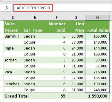
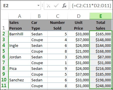
Here we’re calculating Total Sales of coupes and sedans for each salesperson by entering =F10:F19*G10:G19 in cell H10.

When you press Enter, you’ll see the results spill down to cells H10:H19. Notice that the spill range is highlighted with a border when you select any cell within the spill range. You might also notice that the formulas in cells H10:H19 are grayed out. They’re just there for reference, so if you want to adjust the formula, you’ll need to select cell H10, where the master formula lives.
Single-cell array formula

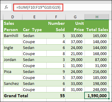
In cell H20 of the example workbook, type or copy and paste =SUM(F10:F19*G10:G19), and then press Enter.

In this case, Excel multiplies the values in the array (the cell range F10 through G19), and then uses the SUM function to add the totals together. The result is a grand total of $1,590,000 in sales.

This example shows how powerful this type of formula can be. For example, suppose you have 1,000 rows of data. You can sum part or all of that data by creating an array formula in a single cell instead of dragging the formula down through the 1,000 rows. Also, notice that the single-cell formula in cell H20 is completely independent of the multi-cell formula (the formula in cells H10 through H19). This is another advantage of using array formulas — flexibility. You could change the other formulas in column H without affecting the formula in H20. It can also be good practice to have independent totals like this, as it helps validate the accuracy of your results.
Dynamic array formulas also offer these advantages:
- Consistency If you click any of the cells from H10 downward, you see the same formula. That consistency can help ensure greater accuracy.
- Safety You can’t overwrite a component of a multi-cell array formula. For example, click cell H11 and press Delete. Excel won’t change the array’s output. To change it, you need to select the top-left cell in the array, or cell H10.
- Smaller file sizes You can often use a single array formula instead of several intermediate formulas. For example, the car sales example uses one array formula to calculate the results in column E. If you had used standard formulas such as =F10*G10, F11*G11, F12*G12, etc., you would have used 11 different formulas to calculate the same results. That’s not a big deal, but what if you had thousands of rows to total? Then it can make a big difference.
- Efficiency Array functions can be an efficient way to build complex formulas. The array formula =SUM(F10:F19*G10:G19) is the same as this: =SUM(F10*G10,F11*G11,F12*G12,F13*G13,F14*G14,F15*G15,F16*G16,F17*G17,F18*G18,F19*G19).
- Spilling Dynamic array formulas will automatically spill into the output range. If your source data is in an Excel table, then your dynamic array formulas will automatically resize as you add or remove data.
- #SPILL! error Dynamic arrays introduced the #SPILL! error, which indicates that the intended spill range is blocked for some reason. When you resolve the blockage, the formula will automatically spill.

Array constants are a component of array formulas. You create array constants by entering a list of items and then manually surrounding the list with braces ({ }), like this:

={1,2,3,4,5} or ={«January»,»February»,»March»}

If you separate the items by using commas, you create a horizontal array (a row). If you separate the items by using semicolons, you create a vertical array (a column). To create a two-dimensional array, you delimit the items in each row with commas, and delimit each row with semicolons.

The following procedures will give you some practice in creating horizontal, vertical, and two-dimensional constants. We’ll show examples using the SEQUENCE function to automatically generate array constants, as well as manually entered array constants.

Create a horizontal constant

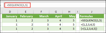
Use the workbook from the previous examples, or create a new workbook. Select any empty cell and enter =SEQUENCE(1,5). The SEQUENCE function builds a 1 row by 5 column array the same as ={1,2,3,4,5}. The following result is displayed:
Create a vertical constant

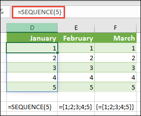
Select any blank cell with room beneath it, and enter =SEQUENCE(5), or ={1;2;3;4;5}. The following result is displayed:
Create a two-dimensional constant

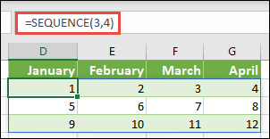
Select any blank cell with room to the right and beneath it, and enter =SEQUENCE(3,4). You see the following result:

You can also enter: or ={1,2,3,4;5,6,7,8;9,10,11,12}, but you’ll want to pay attention to where you put semi-colons versus commas.

As you can see, the SEQUENCE option offers significant advantages over manually entering your array constant values. Primarily, it saves you time, but it can also help reduce errors from manual entry. It’s also easier to read, especially as the semi-colons can be hard to distinguish from the comma separators.

Here’s an example that uses array constants as part of a bigger formula. In the sample workbook, go to the Constant in a formula worksheet, or create a new worksheet.

In cell D9, we entered =SEQUENCE(1,5,3,1), but you could also enter 3, 4, 5, 6, and 7 in cells A9:H9. There’s nothing special about that particular number selection, we just chose something other than 1-5 for differentiation.

In cell E11, enter =SUM(D9:H9*SEQUENCE(1,5)), or =SUM(D9:H9*{1,2,3,4,5}). The formulas return 85.

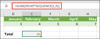
The SEQUENCE function builds the equivalent of the array constant {1,2,3,4,5}. Because Excel performs operations on expressions enclosed in parentheses first, the next two elements that come into play are the cell values in D9:H9, and the multiplication operator (*). At this point, the formula multiplies the values in the stored array by the corresponding values in the constant. It’s the equivalent of:

=SUM(D9*1,E9*2,F9*3,G9*4,H9*5), or =SUM(3*1,4*2,5*3,6*4,7*5)

Finally, the SUM function adds the values, and returns 85.

To avoid using the stored array and keep the operation entirely in memory, you can replace it with another array constant:

=SUM(SEQUENCE(1,5,3,1)*SEQUENCE(1,5)), or =SUM({3,4,5,6,7}*{1,2,3,4,5})

Elements that you can use in array constants

Array constants can contain numbers, text, logical values (such as TRUE and FALSE), and error values such as #N/A. You can use numbers in integer, decimal, and scientific formats. If you include text, you need to surround it with quotation marks («text”).
Array constants can’t contain additional arrays, formulas, or functions. In other words, they can contain only text or numbers that are separated by commas or semicolons. Excel displays a warning message when you enter a formula such as {1,2,A1:D4} or {1,2,SUM(Q2:Z8)}. Also, numeric values can’t contain percent signs, dollar signs, commas, or parentheses.

One of the best ways to use array constants is to name them. Named constants can be much easier to use, and they can hide some of the complexity of your array formulas from others. To name an array constant and use it in a formula, do the following:

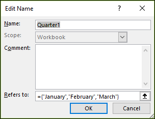
Go to Formulas > Defined Names > Define Name. In the Name box, type Quarter1. In the Refers to box, enter the following constant (remember to type the braces manually):

={«January»,»February»,»March»}

The dialog box should now look like this:

Click OK, then select any row with three blank cells, and enter =Quarter1.

The following result is displayed:

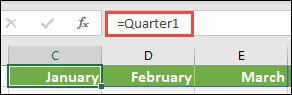
If you want the results to spill vertically instead of horizontally, you can use =TRANSPOSE(Quarter1).

If you want to display a list of 12 months, like you might use when building a financial statement, you can base one off the current year with the SEQUENCE function. The neat thing about this function is that even though only the month is displaying, there is a valid date behind it that you can use in other calculations. You’ll find these examples on the Named array constant and Quick sample dataset worksheets in the example workbook.

=TEXT(DATE(YEAR(TODAY()),SEQUENCE(1,12),1),»mmm»)

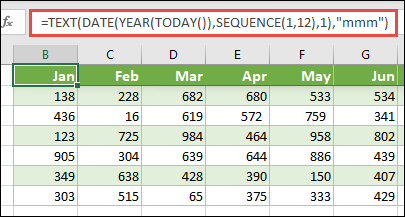
This uses the DATE function to create a date based on the current year, SEQUENCE creates an array constant from 1 to 12 for January through December, then the TEXT function converts the display format to «mmm» (Jan, Feb, Mar, etc.). If you wanted to display the full month name, such as January, you’d use «mmmm».

When you use a named constant as an array formula, remember to enter the equal sign, as in =Quarter1, not just Quarter1. If you don’t, Excel interprets the array as a string of text and your formula won’t work as expected. Finally, keep in mind that you can use combinations of functions, text and numbers. It all depends on how creative you want to get.

The following examples demonstrate a few of the ways in which you can put array constants to use in array formulas. Some of the examples use the TRANSPOSE function to convert rows to columns and vice versa.

Multiple each item in an array

Enter =SEQUENCE(1,12)*2, or ={1,2,3,4;5,6,7,8;9,10,11,12}*2

You can also divide with (/), add with (+), and subtract with (—).
Square the items in an array

Enter =SEQUENCE(1,12)^2, or ={1,2,3,4;5,6,7,8;9,10,11,12}^2
Find the square root of squared items in an array

Enter =SQRT(SEQUENCE(1,12)^2), or =SQRT({1,2,3,4;5,6,7,8;9,10,11,12}^2)
Transpose a one-dimensional row

Enter =TRANSPOSE(SEQUENCE(1,5)), or =TRANSPOSE({1,2,3,4,5})

Even though you entered a horizontal array constant, the TRANSPOSE function converts the array constant into a column.
Transpose a one-dimensional column

Enter =TRANSPOSE(SEQUENCE(5,1)), or =TRANSPOSE({1;2;3;4;5})

Even though you entered a vertical array constant, the TRANSPOSE function converts the constant into a row.
Transpose a two-dimensional constant

Enter =TRANSPOSE(SEQUENCE(3,4)), or =TRANSPOSE({1,2,3,4;5,6,7,8;9,10,11,12})

The TRANSPOSE function converts each row into a series of columns.

This section provides examples of basic array formulas.

Create an array from existing values

The following example explains how to use array formulas to create a new array from an existing array.

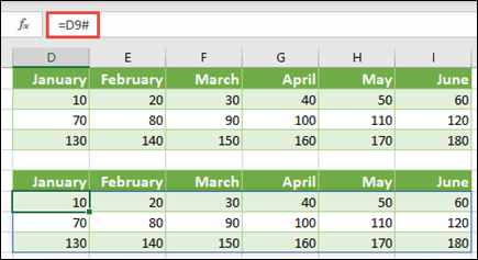
Enter =SEQUENCE(3,6,10,10), or ={10,20,30,40,50,60;70,80,90,100,110,120;130,140,150,160,170,180}

Be sure to type { (opening brace) before you type 10, and } (closing brace) after you type 180, because you’re creating an array of numbers.

Next, enter =D9#, or =D9:I11 in a blank cell. A 3 x 6 array of cells appears with the same values you see in D9:D11. The # sign is called the spilled range operator, and it’s Excel’s way of referencing the entire array range instead of having to type it out.
Create an array constant from existing values

You can take the results of a spilled array formula and convert that into its component parts. Select cell D9, then press F2 to switch to edit mode. Next, press F9 to convert the cell references to values, which Excel then converts into an array constant. When you press Enter, the formula, =D9#, should now be ={10,20,30;40,50,60;70,80,90}.
Count characters in a range of cells

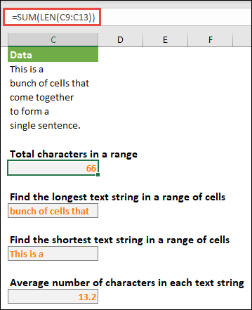
The following example shows you how to count the number of characters in a range of cells. This includes spaces.

=SUM(LEN(C9:C13))

In this case, the LEN function returns the length of each text string in each of the cells in the range. The SUM function then adds those values together and displays the result (66). If you wanted to get average number of characters, you could use:

=AVERAGE(LEN(C9:C13))
Contents of longest cell in range C9:C13

=INDEX(C9:C13,MATCH(MAX(LEN(C9:C13)),LEN(C9:C13),0),1)

This formula works only when a data range contains a single column of cells.

Let’s take a closer look at the formula, starting from the inner elements and working outward. The LEN function returns the length of each of the items in the cell range D2:D6. The MAX function calculates the largest value among those items, which corresponds to the longest text string, which is in cell D3.

Here’s where things get a little complex. The MATCH function calculates the offset (the relative position) of the cell that contains the longest text string. To do that, it requires three arguments: a lookup value, a lookup array, and a match type. The MATCH function searches the lookup array for the specified lookup value. In this case, the lookup value is the longest text string:

MAX(LEN(C9:C13)

and that string resides in this array:

LEN(C9:C13)

The match type argument in this case is 0. The match type can be a 1, 0, or -1 value.
- 1 — returns the largest value that is less than or equal to the lookup val
- 0 — returns the first value exactly equal to the lookup value
- -1 — returns the smallest value that is greater than or equal to the specified lookup value
- If you omit a match type, Excel assumes 1.
Finally, the INDEX function takes these arguments: an array, and a row and column number within that array. The cell range C9:C13 provides the array, the MATCH function provides the cell address, and the final argument (1) specifies that the value comes from the first column in the array.

If you wanted to get the contents of the smallest text string, you would replace MAX in the above example with MIN.
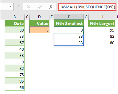
Find the n smallest values in a range

This example shows how to find the three smallest values in a range of cells, where an array of sample data in cells B9:B18has been created with: =INT(RANDARRAY(10,1)*100). Note that RANDARRAY is a volatile function, so you’ll get a new set of random numbers each time Excel calculates.

Enter =SMALL(B9#,SEQUENCE(D9), =SMALL(B9:B18,{1;2;3})

This formula uses an array constant to evaluate the SMALL function three times and return the smallest 3 members in the array that’s contained in cells B9:B18, where 3 is a variable value in cell D9. To find more values, you can increase the value in the SEQUENCE function, or add more arguments to the constant. You can also use additional functions with this formula, such as SUM or AVERAGE. For example:

=SUM(SMALL(B9#,SEQUENCE(D9))

=AVERAGE(SMALL(B9#,SEQUENCE(D9))
Find the n largest values in a range

To find the largest values in a range, you can replace the SMALL function with the LARGE function. In addition, the following example uses the ROW and INDIRECT functions.

Enter =LARGE(B9#,ROW(INDIRECT(«1:3»))), or =LARGE(B9:B18,ROW(INDIRECT(«1:3»)))

At this point, it may help to know a bit about the ROW and INDIRECT functions. You can use the ROW function to create an array of consecutive integers. For example, select an empty and enter:

=ROW(1:10)

The formula creates a column of 10 consecutive integers. To see a potential problem, insert a row above the range that contains the array formula (that is, above row 1). Excel adjusts the row references, and the formula now generates integers from 2 to 11. To fix that problem, you add the INDIRECT function to the formula:

=ROW(INDIRECT(«1:10»))

The INDIRECT function uses text strings as its arguments (which is why the range 1:10 is surrounded by quotation marks). Excel does not adjust text values when you insert rows or otherwise move the array formula. As a result, the ROW function always generates the array of integers that you want. You could just as easily use SEQUENCE:

=SEQUENCE(10)

Let’s examine the formula that you used earlier — =LARGE(B9#,ROW(INDIRECT(«1:3»))) — starting from the inner parentheses and working outward: The INDIRECT function returns a set of text values, in this case the values 1 through 3. The ROW function in turn generates a three-cell column array. The LARGE function uses the values in the cell range B9:B18, and it is evaluated three times, once for each reference returned by the ROW function. If you want to find more values, you add a greater cell range to the INDIRECT function. Finally, as with the SMALL examples, you can use this formula with other functions, such as SUM and AVERAGE.

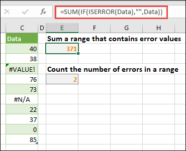
Sum a range that contains error values

The SUM function in Excel does not work when you try to sum a range that contains an error value, such as #VALUE! or #N/A. This example shows you how to sum the values in a range named Data that contains errors:
=SUM(IF(ISERROR(Data),»»,Data))

The formula creates a new array that contains the original values minus any error values. Starting from the inner functions and working outward, the ISERROR function searches the cell range (Data) for errors. The IF function returns a specific value if a condition you specify evaluates to TRUE and another value if it evaluates to FALSE. In this case, it returns empty strings («») for all error values because they evaluate to TRUE, and it returns the remaining values from the range (Data) because they evaluate to FALSE, meaning that they don’t contain error values. The SUM function then calculates the total for the filtered array.
Count the number of error values in a range

This example is like the previous formula, but it returns the number of error values in a range named Data instead of filtering them out:

=SUM(IF(ISERROR(Data),1,0))

This formula creates an array that contains the value 1 for the cells that contain errors and the value 0 for the cells that don’t contain errors. You can simplify the formula and achieve the same result by removing the third argument for the IF function, like this:

=SUM(IF(ISERROR(Data),1))

If you don’t specify the argument, the IF function returns FALSE if a cell does not contain an error value. You can simplify the formula even more:

=SUM(IF(ISERROR(Data)*1))

This version works because TRUE*1=1 and FALSE*1=0.

You might need to sum values based on conditions.

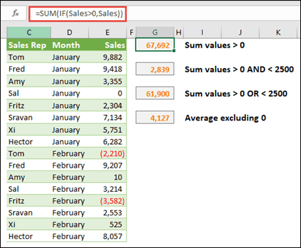
For example, this array formula sums just the positive integers in a range named Sales, which represents cells E9:E24 in the example above:

=SUM(IF(Sales>0,Sales))

The IF function creates an array of positive and false values. The SUM function essentially ignores the false values because 0+0=0. The cell range that you use in this formula can consist of any number of rows and columns.

You can also sum values that meet more than one condition. For example, this array formula calculates values greater than 0 AND less than 2500:

=SUM((Sales>0)*(Sales<2500)*(Sales))

Keep in mind that this formula returns an error if the range contains one or more non-numeric cells.

You can also create array formulas that use a type of OR condition. For example, you can sum values that are greater than 0 OR less than 2500:

=SUM(IF((Sales>0)+(Sales<2500),Sales))

You can’t use the AND and OR functions in array formulas directly because those functions return a single result, either TRUE or FALSE, and array functions require arrays of results. You can work around the problem by using the logic shown in the previous formula. In other words, you perform math operations, such as addition or multiplication on values that meet the OR or AND condition.

This example shows you how to remove zeros from a range when you need to average the values in that range. The formula uses a data range named Sales:

=AVERAGE(IF(Sales<>0,Sales))

The IF function creates an array of values that do not equal 0 and then passes those values to the AVERAGE function.

This array formula compares the values in two ranges of cells named MyData and YourData and returns the number of differences between the two. If the contents of the two ranges are identical, the formula returns 0. To use this formula, the cell ranges need to be the same size and of the same dimension. For example, if MyData is a range of 3 rows by 5 columns, YourData must also be 3 rows by 5 columns:

=SUM(IF(MyData=YourData,0,1))

The formula creates a new array of the same size as the ranges that you are comparing. The IF function fills the array with the value 0 and the value 1 (0 for mismatches and 1 for identical cells). The SUM function then returns the sum of the values in the array.

You can simplify the formula like this:

=SUM(1*(MyData<>YourData))

Like the formula that counts error values in a range, this formula works because TRUE*1=1, and FALSE*1=0.

This array formula returns the row number of the maximum value in a single-column range named Data:

=MIN(IF(Data=MAX(Data),ROW(Data),»»))

The IF function creates a new array that corresponds to the range named Data. If a corresponding cell contains the maximum value in the range, the array contains the row number. Otherwise, the array contains an empty string («»). The MIN function uses the new array as its second argument and returns the smallest value, which corresponds to the row number of the maximum value in Data. If the range named Data contains identical maximum values, the formula returns the row of the first value.

If you want to return the actual cell address of a maximum value, use this formula:

=ADDRESS(MIN(IF(Data=MAX(Data),ROW(Data),»»)),COLUMN(Data))

You’ll find similar examples in the sample workbook on the Differences between datasets worksheet.

Multi-cell array formula

Copy the entire table below and paste it into cell A1 in a blank worksheet.

Sales Person	Car Type	Number Sold	Unit Price
Barnhill	Sedan	5	33000
	Coupe	4	37000
Ingle	Sedan	6	24000
	Coupe	8	21000
Jordan	Sedan	3	29000
	Coupe	1	31000
Pica	Sedan	9	24000
	Coupe	5	37000
Sanchez	Sedan	6	33000
	Coupe	8	31000
Formula (Grand Total)			Grand Total
‘=SUM(C2:C11*D2:D11)			=SUM(C2:C11*D2:D11)

To see Total Sales of coupes and sedans for each salesperson, select cells E2:E11, enter the formula =C2:C11*D2:D11, and then press Ctrl+Shift+Enter.
To see the Grand Total of all sales, select cell F11, enter the formula =SUM(C2:C11*D2:D11), and then press Ctrl+Shift+Enter.

When you press Ctrl+Shift+Enter, Excel surrounds the formula with braces ({ }) and inserts an instance of the formula in each cell of the selected range. This happens very quickly, so what you see in column E is the total sales amount for each car type for each salesperson. If you select E2, then select E3, E4, and so on, you’ll see that the same formula is shown: {=C2:C11*D2:D11}.

Create a single-cell array formula

In cell D13 of the workbook, type the following formula, and then press Ctrl+Shift+Enter:

=SUM(C2:C11*D2:D11)

In this case, Excel multiplies the values in the array (the cell range C2 through D11) and then uses the SUM function to add the totals together. The result is a grand total of $1,590,000 in sales. This example shows how powerful this type of formula can be. For example, suppose you have 1,000 rows of data. You can sum part or all of that data by creating an array formula in a single cell instead of dragging the formula down through the 1,000 rows.

Also, notice that the single-cell formula in cell D13 is completely independent of the multi-cell formula (the formula in cells E2 through E11). This is another advantage of using array formulas — flexibility. You could change the formulas in column E or delete that column altogether, without affecting the formula in D13.

Array formulas also offer these advantages:

Consistency If you click any of the cells from E2 downward, you see the same formula. That consistency can help ensure greater accuracy.
Safety You cannot overwrite a component of a multi-cell array formula. For example, click cell E3 and press Delete. You have to either select the entire range of cells (E2 through E11) and change the formula for the entire array, or leave the array as is. As an added safety measure, you have to press Ctrl+Shift+Enter to confirm any change to the formula.
Smaller file sizes You can often use a single array formula instead of several intermediate formulas. For example, the workbook uses one array formula to calculate the results in column E. If you had used standard formulas (such as =C2*D2, C3*D3, C4*D4…), you would have used 11 different formulas to calculate the same results.

In general, array formulas use standard formula syntax. They all begin with an equal (=) sign, and you can use most of the built-in Excel functions in your array formulas. The key difference is that when using an array formula, you press Ctrl+Shift+Enter to enter your formula. When you do this, Excel surrounds your array formula with braces — if you type the braces manually, your formula will be converted to a text string, and it won’t work.

Array functions can be an efficient way to build complex formulas. The array formula =SUM(C2:C11*D2:D11) is the same as this: =SUM(C2*D2,C3*D3,C4*D4,C5*D5,C6*D6,C7*D7,C8*D8,C9*D9,C10*D10,C11*D11).

Important: Press Ctrl+Shift+Enter whenever you need to enter an array formula. This applies to both single-cell and multi-cell formulas.

Whenever you work with multi-cell formulas, also remember:

Select the range of cells to hold your results before you enter the formula. You did this when you created the multi-cell array formula when you selected cells E2 through E11.
You can’t change the contents of an individual cell in an array formula. To try this, select cell E3 in the workbook and press Delete. Excel displays a message that tells you that you can’t change part of an array.
You can move or delete an entire array formula, but you can’t move or delete part of it. In other words, to shrink an array formula, you first delete the existing formula and then start over.
To delete an array formula, select the entire formula range (for example, E2:E11), then press Delete.
You can’t insert blank cells into, or delete cells from a multi-cell array formula.

At times, you may need to expand an array formula. Select the first cell in existing array range, and continue until you’ve selected the entire range that you want to extend the formula to. Press F2 to edit the formula, then press CTRL+SHIFT+ENTER to confirm the formula once you’ve adjusted the formula range. The key is to select the entire range, starting with the top-left cell in the array. The top-left cell is the one that gets edited.

Array formulas are great, but they can have some disadvantages:

You may occasionally forget to press Ctrl+Shift+Enter. It can happen to even the most experienced Excel users. Remember to press this key combination whenever you enter or edit an array formula.
Other users of your workbook might not understand your formulas. In practice, array formulas are generally not explained in a worksheet. Therefore, if other people need to modify your workbooks, you should either avoid array formulas or make sure those people know about any array formulas and understand how to change them, if they need to.
Depending on the processing speed and memory of your computer, large array formulas can slow down calculations.

Array constants are a component of array formulas. You create array constants by entering a list of items and then manually surrounding the list with braces ({ }), like this:

={1,2,3,4,5}

By now, you know you need to press Ctrl+Shift+Enter when you create array formulas. Because array constants are a component of array formulas, you surround the constants with braces by manually typing them. You then use Ctrl+Shift+Enter to enter the entire formula.

Here’s an array in a single row: {1,2,3,4}. Here’s an array in a single column: {1;2;3;4}. And here’s an array of two rows and four columns: {1,2,3,4;5,6,7,8}. In the two row array, the first row is 1, 2, 3, and 4, and the second row is 5, 6, 7, and 8. A single semicolon separates the two rows, between 4 and 5.

As with array formulas, you can use array constants with most of the built-in functions that Excel provides. The following sections explain how to create each kind of constant and how to use these constants with functions in Excel.

The following procedures will give you some practice in creating horizontal, vertical, and two-dimensional constants.

Create a horizontal constant

In a blank worksheet, select cells A1 through E1.
In the formula bar, enter the following formula, and then press Ctrl+Shift+Enter:

={1,2,3,4,5}

In this case, you should type the opening and closing braces ({ }), and Excel will add the second set for you.

The following result is displayed.

Create a vertical constant

In your workbook, select a column of five cells.
In the formula bar, enter the following formula, and then press Ctrl+Shift+Enter:

={1;2;3;4;5}

The following result is displayed.

Create a two-dimensional constant

In your workbook, select a block of cells four columns wide by three rows high.
In the formula bar, enter the following formula, and then press Ctrl+Shift+Enter:

={1,2,3,4;5,6,7,8;9,10,11,12}

You see the following result:

Use constants in formulas

Here is a simple example that uses constants:

In the sample workbook, create a new worksheet.
In cell A1, type 3, and then type 4 in B1, 5 in C1, 6 in D1, and 7 in E1.
In cell A3, type the following formula, and then press Ctrl+Shift+Enter:

=SUM(A1:E1*{1,2,3,4,5})

Notice that Excel surrounds the constant with another set of braces, because you entered it as an array formula.

The value 85 appears in cell A3.

The next section explains how the formula works.

The formula you just used contains several parts.

1. Function

2. Stored array

3. Operator

4. Array constant

The last element inside the parentheses is the array constant: {1,2,3,4,5}. Remember that Excel does not surround array constants with braces; you actually type them. Also remember that after you add a constant to an array formula, you press Ctrl+Shift+Enter to enter the formula.

Because Excel performs operations on expressions enclosed in parentheses first, the next two elements that come into play are the values stored in the workbook (A1:E1) and the operator. At this point, the formula multiplies the values in the stored array by the corresponding values in the constant. It’s the equivalent of:

=SUM(A1*1,B1*2,C1*3,D1*4,E1*5)

Finally, the SUM function adds the values, and the sum 85 appears in cell A3.

To avoid using the stored array and to just keep the operation entirely in memory, replace the stored array with another array constant:

=SUM({3,4,5,6,7}*{1,2,3,4,5})

To try this, copy the function, select a blank cell in your workbook, paste the formula into the formula bar, and then press Ctrl+Shift+Enter. You’ll see the same result as you did in the earlier exercise that used the array formula:

=SUM(A1:E1*{1,2,3,4,5})

Array constants can contain numbers, text, logical values (such as TRUE and FALSE), and error values ( such as #N/A). You can use numbers in the integer, decimal, and scientific formats. If you include text, you need to surround the text with quotation marks («).

Array constants can’t contain additional arrays, formulas, or functions. In other words, they can contain only text or numbers that are separated by commas or semicolons. Excel displays a warning message when you enter a formula such as {1,2,A1:D4} or {1,2,SUM(Q2:Z8)}. Also, numeric values can’t contain percent signs, dollar signs, commas, or parentheses.

One of the best way to use array constants is to name them. Named constants can be much easier to use, and they can hide some of the complexity of your array formulas from others. To name an array constant and use it in a formula, do the following:

On the Formulas tab, in the Defined Names group, click Define Name.
The Define Name dialog box appears.
In the Name box, type Quarter1.
In the Refers to box, enter the following constant (remember to type the braces manually):

={«January»,»February»,»March»}

The contents of the dialog box now looks like this:
Click OK, and then select a row of three blank cells.
Type the following formula, and then press Ctrl+Shift+Enter.

=Quarter1

The following result is displayed.

When you use a named constant as an array formula, remember to enter the equal sign. If you don’t, Excel interprets the array as a string of text and your formula won’t work as expected. Finally, keep in mind that you can use combinations of text and numbers.

Look for the following problems when your array constants don’t work:

Some elements might not be separated with the proper character. If you omit a comma or semicolon, or if you put one in the wrong place, the array constant might not be created correctly, or you might see a warning message.
You might have selected a range of cells that doesn’t match the number of elements in your constant. For example, if you select a column of six cells for use with a five-cell constant, the #N/A error value appears in the empty cell. Conversely, if you select too few cells, Excel omits the values that don’t have a corresponding cell.

Multiply each item in an array

Create a new worksheet, and then select a block of empty cells four columns wide by three rows high.
Type the following formula, and then press Ctrl+Shift+Enter:

={1,2,3,4;5,6,7,8;9,10,11,12}*2

Square the items in an array

Select a block of empty cells four columns wide by three rows high.
Type the following array formula, and then press Ctrl+Shift+Enter:

={1,2,3,4;5,6,7,8;9,10,11,12}*{1,2,3,4;5,6,7,8;9,10,11,12}

Alternatively, enter this array formula, which uses the caret operator (^):

={1,2,3,4;5,6,7,8;9,10,11,12}^2

Transpose a one-dimensional row

Select a column of five blank cells.
Type the following formula, and then press Ctrl+Shift+Enter:

=TRANSPOSE({1,2,3,4,5})

Even though you entered a horizontal array constant, the TRANSPOSE function converts the array constant into a column.

Transpose a one-dimensional column

Select a row of five blank cells.
Enter the following formula, and then press Ctrl+Shift+Enter:

=TRANSPOSE({1;2;3;4;5})

Even though you entered a vertical array constant, the TRANSPOSE function converts the constant into a row.

Transpose a two-dimensional constant

Select a block of cells three columns wide by four rows high.
Enter the following constant, and then press Ctrl+Shift+Enter:

=TRANSPOSE({1,2,3,4;5,6,7,8;9,10,11,12})

The TRANSPOSE function converts each row into a series of columns.

This section provides examples of basic array formulas.

Create arrays and array constants from existing values

The following example explains how to use array formulas to create links between ranges of cells in different worksheets. It also shows you how to create an array constant from the same set of values.

Create an array from existing values

On a worksheet in Excel, select cells C8:E10, and enter this formula:

={10,20,30;40,50,60;70,80,90}

Be sure to type { (opening brace) before you type 10, and } (closing brace) after you type 90, because you’re creating an array of numbers.
Press Ctrl+Shift+Enter, which enters this array of numbers in the cell range C8:E10 by using an array formula. On your worksheet, C8 through E10 should look like this:

10

20

30

40

50

60

70

80

90
Select the cell range C1 through E3.
Enter the following formula in the formula bar, and then press Ctrl+Shift+Enter:

=C8:E10

A 3×3 array of cells appears in cells C1 through E3 with the same values you see in C8 through E10.

10	20	30
40	50	60
70	80	90

Create an array constant from existing values

With cells C1:C3 selected, press F2 to switch to edit mode.
Press F9 to convert the cell references to values. Excel converts the values into an array constant. The formula should now be ={10,20,30;40,50,60;70,80,90}.
Press Ctrl+Shift+Enter to enter the array constant as an array formula.

Count characters in a range of cells

The following example shows you how to count the number of characters, including spaces, in a range of cells.

Copy this entire table and paste into a worksheet in cell A1.

Data
This is a
bunch of cells that
come together
to form a
single sentence.

Total characters in A2:A6
=SUM(LEN(A2:A6))

Contents of longest cell (A3)
=INDEX(A2:A6,MATCH(MAX(LEN(A2:A6)),LEN(A2:A6),0),1)

Select cell A8, and then press Ctrl+Shift+Enter to see the total number of characters in cells A2:A6 (66).
Select cell A10, and then press Ctrl+Shift+Enter to see the contents of the longest of cells A2:A6 (cell A3).

The following formula is used in cell A8 counts the total number of characters (66) in cells A2 through A6.

=SUM(LEN(A2:A6))

In this case, the LEN function returns the length of each text string in each of the cells in the range. The SUM function then adds those values together and displays the result (66).

Find the n smallest values in a range

This example shows how to find the three smallest values in a range of cells.

Enter some random numbers in cells A1:A11.
Select cells C1 through C3. This set of cells will hold the results returned by the array formula.
Enter the following formula, and then press Ctrl+Shift+Enter:

=SMALL(A1:A11,{1;2;3})

This formula uses an array constant to evaluate the SMALL function three times and return the smallest (1), second smallest (2), and third smallest (3) members in the array that is contained in cells A1:A10 To find more values, you add more arguments to the constant. You can also use additional functions with this formula, such as SUM or AVERAGE. For example:

=SUM(SMALL(A1:A10,{1,2,3})

=AVERAGE(SMALL(A1:A10,{1,2,3})

Find the n largest values in a range

To find the largest values in a range, you can replace the SMALL function with the LARGE function. In addition, the following example uses the ROW and INDIRECT functions.

Select cells D1 through D3.
In the formula bar, enter this formula, and then press Ctrl+Shift+Enter:

=LARGE(A1:A10,ROW(INDIRECT(«1:3»)))

At this point, it may help to know a bit about the ROW and INDIRECT functions. You can use the ROW function to create an array of consecutive integers. For example, select an empty column of 10 cells in your practice workbook, enter this array formula, and then press Ctrl+Shift+Enter:

=ROW(1:10)

The formula creates a column of 10 consecutive integers. To see a potential problem, insert a row above the range that contains the array formula (that is, above row 1). Excel adjusts the row references, and the formula generates integers from 2 to 11. To fix that problem, you add the INDIRECT function to the formula:

=ROW(INDIRECT(«1:10»))

The INDIRECT function uses text strings as its arguments (which is why the range 1:10 is surrounded by double quotation marks). Excel does not adjust text values when you insert rows or otherwise move the array formula. As a result, the ROW function always generates the array of integers that you want.

Let’s take a look at the formula that you used earlier — =LARGE(A5:A14,ROW(INDIRECT(«1:3»))) — starting from the inner parentheses and working outward: The INDIRECT function returns a set of text values, in this case the values 1 through 3. The ROW function in turn generates a three-cell columnar array. The LARGE function uses the values in the cell range A5:A14, and it is evaluated three times, once for each reference returned by the ROW function. The values 3200, 2700, and 2000 are returned to the three-cell columnar array. If you want to find more values, you add a greater cell range to the INDIRECT function.

As with earlier examples, you can use this formula with other functions, such as SUM and AVERAGE.

Find the longest text string in a range of cells

Go back to the earlier text string example, enter the following formula in an empty cell, and press Ctrl+Shift+Enter:

=INDEX(A2:A6,MATCH(MAX(LEN(A2:A6)),LEN(A2:A6),0),1)

The text «bunch of cells that» appears.

Let’s take a closer look at the formula, starting from the inner elements and working outward. The LEN function returns the length of each of the items in the cell range A2:A6. The MAX function calculates the largest value among those items, which corresponds to the longest text string, which is in cell A3.

Here’s where things get a little complex. The MATCH function calculates the offset (the relative position) of the cell that contains the longest text string. To do that, it requires three arguments: a lookup value, a lookup array, and a match type. The MATCH function searches the lookup array for the specified lookup value. In this case, the lookup value is the longest text string:

(MAX(LEN(A2:A6))

and that string resides in this array:

LEN(A2:A6)

The match type argument is 0. The match type can consist of a 1, 0, or -1 value. If you specify 1, MATCH returns the largest value that is less than or equal to the lookup value. If you specify 0, MATCH returns the first value exactly equal to the lookup value. If you specify -1, MATCH finds the smallest value that is greater than or equal to the specified lookup value. If you omit a match type, Excel assumes 1.

Finally, the INDEX function takes these arguments: an array, and a row and column number within that array. The cell range A2:A6 provides the array, the MATCH function provides the cell address, and the final argument (1) specifies that the value comes from the first column in the array.

This section provides examples of advanced array formulas.

Sum a range that contains error values

The SUM function in Excel does not work when you try to sum a range that contains an error value, such as #N/A. This example shows you how to sum the values in a range named Data that contains errors.

=SUM(IF(ISERROR(Data),»»,Data))

The formula creates a new array that contains the original values minus any error values. Starting from the inner functions and working outward, the ISERROR function searches the cell range (Data) for errors. The IF function returns a specific value if a condition you specify evaluates to TRUE and another value if it evaluates to FALSE. In this case, it returns empty strings («») for all error values because they evaluate to TRUE, and it returns the remaining values from the range (Data) because they evaluate to FALSE, meaning that they don’t contain error values. The SUM function then calculates the total for the filtered array.

Count the number of error values in a range

This example is similar to the previous formula, but it returns the number of error values in a range named Data instead of filtering them out:

=SUM(IF(ISERROR(Data),1,0))

This formula creates an array that contains the value 1 for the cells that contain errors and the value 0 for the cells that don’t contain errors. You can simplify the formula and achieve the same result by removing the third argument for the IF function, like this:

=SUM(IF(ISERROR(Data),1))

If you don’t specify the argument, the IF function returns FALSE if a cell does not contain an error value. You can simplify the formula even more:

=SUM(IF(ISERROR(Data)*1))

This version works because TRUE*1=1 and FALSE*1=0.

Sum values based on conditions

You might need to sum values based on conditions. For example, this array formula sums just the positive integers in a range named Sales:

=SUM(IF(Sales>0,Sales))

The IF function creates an array of positive values and false values. The SUM function essentially ignores the false values because 0+0=0. The cell range that you use in this formula can consist of any number of rows and columns.

You can also sum values that meet more than one condition. For example, this array formula calculates values greater than 0 and less than or equal to 5:

=SUM((Sales>0)*(Sales<=5)*(Sales))

Keep in mind that this formula returns an error if the range contains one or more non-numeric cells.

You can also create array formulas that use a type of OR condition. For example, you can sum values that are less than 5 and greater than 15:

=SUM(IF((Sales<5)+(Sales>15),Sales))

The IF function finds all values smaller than 5 and greater than 15 and then passes those values to the SUM function.

You can’t use the AND and OR functions in array formulas directly because those functions return a single result, either TRUE or FALSE, and array functions require arrays of results. You can work around the problem by using the logic shown in the previous formula. In other words, you perform math operations, such as addition or multiplication, on values that meet the OR or AND condition.

Compute an average that excludes zeros

This example shows you how to remove zeros from a range when you need to average the values in that range. The formula uses a data range named Sales:

=AVERAGE(IF(Sales<>0,Sales))

The IF function creates an array of values that do not equal 0 and then passes those values to the AVERAGE function.

Count the number of differences between two ranges of cells

This array formula compares the values in two ranges of cells named MyData and YourData and returns the number of differences between the two. If the contents of the two ranges are identical, the formula returns 0. To use this formula, the cell ranges need to be the same size and of the same dimension (for example, if MyData is a range of 3 rows by 5 columns, YourData must also be 3 rows by 5 columns):

=SUM(IF(MyData=YourData,0,1))

The formula creates a new array of the same size as the ranges that you are comparing. The IF function fills the array with the value 0 and the value 1 (0 for mismatches and 1 for identical cells). The SUM function then returns the sum of the values in the array.

You can simplify the formula like this:

=SUM(1*(MyData<>YourData))

Like the formula that counts error values in a range, this formula works because TRUE*1=1, and FALSE*1=0.

Find the location of the maximum value in a range

This array formula returns the row number of the maximum value in a single-column range named Data:

=MIN(IF(Data=MAX(Data),ROW(Data),»»))

The IF function creates a new array that corresponds to the range named Data. If a corresponding cell contains the maximum value in the range, the array contains the row number. Otherwise, the array contains an empty string («»). The MIN function uses the new array as its second argument and returns the smallest value, which corresponds to the row number of the maximum value in Data. If the range named Data contains identical maximum values, the formula returns the row of the first value.

If you want to return the actual cell address of a maximum value, use this formula:

=ADDRESS(MIN(IF(Data=MAX(Data),ROW(Data),»»)),COLUMN(Data))

Acknowledgement

Parts of this article were based on a series of Excel Power User columns written by Colin Wilcox, and adapted from chapters 14 and 15 of Excel 2002 Formulas, a book written by John Walkenbach, a former Excel MVP.

Need more help?

You can always ask an expert in the Excel Tech Community or get support in the Answers community.

Watch the Intro Video

Entering and Identifying an Array Formula

When using an Array Formula, you press Ctrl+Shift+Enter instead of just Enter after entering or editing the formula. This is why array formulas are often called CSE formulas.
An Array Formula will show curly brackets or braces around the formula in the Formula Bar like this: {=SUM(A1:A5*B1:B5)}
Array Constants (arrays «hard-coded» into formulas) are enclosed in braces { } and use commas to separate columns, and semi-colons to separate rows, like this 2×3 array: {1, 1, 1; 2, 2, 2}
If an Array Formula returns more than one value (a multi-cell array formula), first select a range of cells equal to size of the returned array, then enter your formula.
To select all the cells within a multi-cell array: Press F5 > Special > Current Array.

! Every time you edit an Array Formula, you must remember to press Ctrl+Shift+Enter afterward. If you forget to, the formula may return an error without you realizing it.

NOTE Google Sheets uses the ARRAYFORMULA function instead of showing the formula surrounded by braces. It is not necessary to press Ctrl+Shift+Enter in Google Sheets, but if you do, ARRAYFORMULA( is added to the beginning of the formula.

Using Array Constants in Formulas

Many functions allow you use array constants like {1,2,6,12} as arguments within formulas. An example that I often use in my yearly calendar templates returns the weekday abbreviation for a given date. The nice thing about this formula is that you can choose whether to display a single character or two characters.

=INDEX({"Su";"M";"Tu";"W";"Th";"F";"Sa"},WEEKDAY(theDate,1))

This formula is not technically an Array Formula because you don’t enter it using Ctrl+Shift+Enter. Using a hard-coded array within a formula does not necessarily require using Ctrl+Shift+Enter.

TIP If you are going to use the array constant in multiple formulas, you may want to first create a Named Constant. Go to Formulas > Name Manager > New Name, enter a descriptive name like payment_frequency and enter ={1,2,6,12} into the Refers To field. You can use the name within your formulas. If you ever want to change the values within that array constant, you only need to change it one place (within the Name Manager).

A Simple Array Formula Example

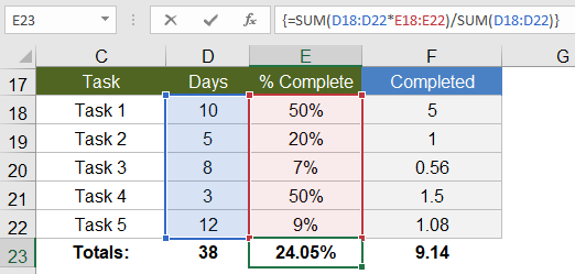
To start out, I will show how an array formula works using a very basic example. Let’s say that I have a list of tasks, the number of days each of those tasks will take, and a column for the percent complete. I want to know the total number of days that have been completed.

Without an array formula, you would create another column called «Completed» and multiply the number of days by the % complete, and copy the formula down. Then I would use SUM to total the number of days completed, like the image below:

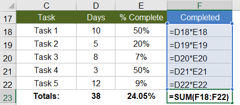
With an array formula, you can do essentially the same thing without having to create the extra column. Within a single cell, you can calculate the total days completed as =SUM(D18:D22*E18:E22), remembering to press Ctrl+Shift+Enter because it is an array formula.

{ =SUM(D18:D22*E18:E22) }

Evaluation Steps
Step 1: =SUM( {10;5;8;3;12} * {0.5;0.2;0.07;0.5;0.09} )
Step 2: =SUM( {10*0.5;5*0.2;8*0.7;3*0.5;12*0.09} )
Step 3: =SUM( {5;1;0.56;1.5;1.08} )
Step 4: =9.14

In this and other examples, I’ve shown the evaluation steps below the formula so that you can see how the formula works. You don’t actually type the curly brackets { }, but in this article I will surround all array formulas with brackets to indicate that they are entered as CSE formulas.

In the evaluation steps shown in the above example, you’ll see that Excel is multiplying each element of the first array by the corresponding element in the second array, and then SUM adds the results.

NOTE It turns out that this particular example can be used to show how the SUMPRODUCT function works, but the SUMPRODUCT function deserves its own article.

To take this example just a bit further, if all we wanted to know was the Total Percent Complete for the entire project, we can divide the total days completed (9.14) by the total days (38) all within a single array formula, and we don’t need column F at all (as shown in the image below).

This example is an example of a single-cell array formula, meaning that the formula is entered into a single cell.

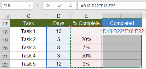
Entering a Multi-Cell Array Formula

Whenever your array formula returns more than one value, if you want to display more than just the first value, you need to select the range of cells that will contain the resulting array before entering your formula. Doing this will result in a multi-cell array formula, meaning that the result of the formula is a multi-cell array.

Using the same example as above, we could use an array formula in the Completed column to calculate Days * Percent Complete. First, select cells F18:F22, then press = and enter the formula, followed by Ctrl+Shift+Enter (CSE). The image below is what it will look like just before you press CSE.

You can edit a multi-cell array formula by selecting any of the cells in the array and then updating the formula and pressing Ctrl+Shift+Enter when you are done. However, you can’t use this technique to modify the size of the array.

«You can’t change part of an array» — This is the warning or error you will get if you try to insert rows or columns or change individual cells within a multi-cell array.

Using multi-cell array formulas can make it more difficult to customize a spreadsheet because to change the size of the array requires that you (1) delete the formula (after selecting all the cells of the array), (2) select the new range of cells, and (3) re-enter the array formula. TIP: Make sure to copy your original formula before deleting it. Then, when you re-enter the formula, you can paste it and modify the ranges.

Nested IF Array Formulas

A nested IF array formula can be very powerful and is probably one of the more common uses for array formulas in Excel. Although Excel provides the SUMIF and COUNTIF and AVERAGEIF functions, they don’t allow as much freedom as a nested IF array formula.

MAX-IF Array Formula

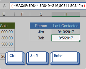
Older versions of Excel do not have the MAXIFS or MINIFS functions, so let’s create our own MAX-IF formula. When we use hyphens to name a formula, it usually means that we’re nesting the functions (IF within MAX in this case).

Let’s say that I have the following contact and sales log and I want a formula that will tell me when I last contacted Bob (cell H51).

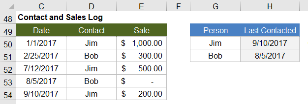
Using MAX on the date range will give me that latest date (9/10/2017), but I only want to include the rows where the contact is Bob. So, I’ll use the MAX-IF array formula:

{ =MAX(IF(contact_range="Bob",date_range)) }

Evaluation Steps
Step 1: =MAX(IF({"Jim";"Bob";"Jim";"Bob";"Jim"}="Bob", date_range ))
Step 2: =MAX(IF({FALSE;TRUE;FALSE;TRUE;FALSE}, date_range ))
Step 3: =MAX( {FALSE,2/25/2017,FALSE,8/5/2017,FALSE} )
Step 4: =8/5/2017

LARGE-IF Array Formula

The LARGE and SMALL functions come in handy when you want to find the value that is perhaps the 2nd largest or 2nd smallest.

The following function will return the second largest sale where the contact is Jim.

{ =LARGE(IF(contact_range="Jim",sale_range),2) }

SMALL-IF Array Formula

This function returns the second smallest sale where the contact is Jim.

{ =SMALL(IF(contact_range="Jim",date_range),2) }

The LARGE and SMALL functions can be used for sorting arrays. More on that later. Hopefully, Excel will introduce a SORT function soon (Google Sheets has already done that).

The SMALL-IF formula can be used in combination with INDEX to do a lookup a value based on the Nth Match.

SUM-IF Array Formula

Yes, there is already a SUMIF function that is generally better than using an array formula, but we’ll be getting into more advanced SUM-IF array formulas, so it’s useful to see the simple example:

{ =SUM(IF(contact_range="Jim",sales_range)) }

More Reading: Chip Pearson provides some great examples of ways to use nested IF functions within the SUM and AVERAGE functions to ignore errors and zero values. See Chip Pearson’s article.

COUNTIF Alternative: SUM-Boolean Array Formulas

Although there is already a COUNTIF function, the criteria available in the COUNTIF family of functions is limited. An alternative method is to do a SUM of boolean (TRUE/FALSE) results that have been converted to 0s and 1s (FALSE=0, TRUE=1). Boolean results can be converted to 0s and 1s by adding +0, multiplying by *1 and by using double negation.

SUM-ISERROR: Count the number of Error values in a range

{ =SUM(1*ISERROR(range)) }
{ =SUM(0+ISERROR(range)) }
{ =SUM(--ISERROR(range)) }

Evaluation Steps
Step 1: =SUM( 1*{FALSE,TRUE,TRUE,FALSE,TRUE} )
Step 2: =SUM( {0,1,1,0,1} )
Step 3: =3

SUM-ISBLANK: Count the number of Blank values in a range

{ =SUM(--ISBLANK(range)) }

Remember: A formula that returns an empty «» string is considered NOT blank.

SUM-NOT-ISBLANK: Count the number of Non-Blank values in a range

{ =SUM(--NOT(ISBLANK(range)) }

Multi-Criteria Boolean Array Formulas

The AND and OR functions return only a single value, even when they contain multiple arrays, so we don’t generally use them within array formulas.

For multiple-criteria logical array formulas, such as SUM-IF between two dates, you need to do the boolean logic by adding boolean values for «or» conditions and by multiplying boolean values for «and» conditions.

SUM-IF Between Two Dates

Yes, SUMIFS would be easier, but let’s assume we are using an older version of Excel. Referring back to the Contact and Sales log, we’ll sum all of the Sales between 2/1/2017 and 9/1/2017, meaning that Date >= 2/1/2017 AND Date <= 9/1/2017.

{ =SUM(IF((date_range>=start)*(date_range<=end), sum_range) ) }

Evaluation Steps
Step 1: SUM(IF({FALSE,TRUE,TRUE,TRUE,TRUE}*{TRUE,TRUE,TRUE,TRUE,FALSE},sum_range))
Step 2: SUM(IF({0,1,1,1,0},sum_range))
Step 3: SUM({FALSE,300,500,0,FALSE})
Step 4: 800

In this case we don’t need to use 1*(…) to convert the boolean values, because the boolean values are converted to 0s and 1s automatially when we multiply the two arrays together. The IF function in Excel treats the value 0 as FALSE and all other values as TRUE.

Overlapping OR Conditions

To demonstrate a logical OR condition, we’ll sum the sales where Name = «Bob» OR Date > 7/1/2017. An «or» condition is true when one or more of the conditions is true, so we check whether the sum of the expressions is greater than 0.

{ =SUM(IF( ((contact_range="Bob")+(date_range>=date))>0, sum_range) ) }

Evaluation Steps
Step 1: SUM(IF(({FALSE,TRUE,FALSE,TRUE,FALSE}+{FALSE,FALSE,TRUE,TRUE,TRUE})>0,sum_range))
Step 2: SUM(IF({0,1,1,2,1}>0,sum_range))
Step 3: SUM(IF({FALSE,TRUE,TRUE,TRUE,TRUE},sum_range))
Step 4: SUM({FALSE,300,500,0,200})
Step 5: 1000

Using this approach, you can create multiple-criteria equivalents for MAX-IF, LARGE-IF, and other array formulas.

Sequential Number Arrays

For many array formulas, you will need to use an array of sequential numbers like {1; 2; 3; … n}. You can return a sequential number array from 1 to n using this formula:

{ =ROW(1:n) }
-or-
{ =ROW(OFFSET($A$1,0,0,n,1)) }

Important: Although it doesn’t matter what is contained in cell A1, if you delete the cell (by removing row 1 or column A for example), insert a row above or a column to the left of cell A1, or cut and paste cell A1 to a different location, your array formula will be messed up. To avoid this problem, use the INDIRECT function:

{ =ROW(INDIRECT("1:"&n)) }
-or-
{ ROW(OFFSET(INDIRECT("A1"),0,0,n,1)) }

NOTE The OFFSET and INDIRECT function are volatile functions. If calculation speed becomes a problem due to these formulas, you could either use ROW(1:n) and risk having row 1 removed, or you could reference a hidden or protected worksheet using =ROW(Sheet4!1:n)

Variant #1: Create a Sequence of Whole Numbers from i to j

If you want to hard-code the values for i and j into the formula, an array formula such as ROW(4:8) may work fine to create the array {4;5;6;7;8}. If you want the formula to use cell references for i and j, you can use INDIRECT like this:

A1 = 4
B1 = 8
{ =ROW(INDIRECT(A1&":"&B1)) }

Result: {4;5;6;7;8}

Variant #2: Create an n x 1 Vector of Whole Numbers Starting From s

You can use this technique when you want to specify the length of the number array instead of the end value. To create the array {s; s+1; s+2; … s+n-1} use

s = 4
n = 7
{ =s+ROW(OFFSET(INDIRECT("A1"),0,0,n,1))-1 }
   -or-
{ =ROW(INDIRECT(s&":"&s+n-1)) }

Result: {4;5;6;7;8;9;10}

Variant #3: Sequence of Dates Between START and END (inclusive)

To create an array of dates from start through end (assuming start and end are cells containing date values), remember that date values are stored as whole numbers. If they are indeed date values and not date-time values, you can use:

start_date = 1/1/2018
end_date = 1/5/2018
{ =ROW(INDIRECT(start_date&":"&end_date)) }

Result: {43101;43102;43103;43104;43105}

The result shows the numeric values for 1/1/2018, 1/2/2018, etc. You can format the results using whatever date format you want. If your start and end dates might be date-time values, then strip the time portion off of the number like this:

{ =ROW(INDIRECT(INT(start_date)&":"&INT(end_date)) }

Variant #4: Create an n x 1 Vector of Sequential Powers of 10

To create the array {1; 10; 100; 1000; … 10^(n-1)} use

{ =10^(ROW(OFFSET(INDIRECT("A1"),0,0,n,1))-1) }
-or-
{ =10^(ROW(INDIRECT("1:"&n))-1) }

Formulas for Matrices

Excel contains some key functions for working with matrices:

MUNIT(m): Creates an Identity matrix of size m x m
MMULT(A,B): Uses matrix multiplication to multiply an n x k matrix A by a k x m matrix B resulting in an array of size n x m.
TRANSPOSE(A): Switches rows to columns or vice versa, and can be used for more than just numbers.
MDETERM(A): Calculates the determinant of a matrix A.
MINVERSE(A): Calculates the inverse of the matrix A (if possible).
INDEX(A,n) or INDEX(A,0,m): Returns either row n or column m of matrix A.

NOTE Excel does a great job of displaying data, but if you need to do a lot of statistical analysis and linear algebra, other tools such as Python, R, and Matlab may be better.

Element-Wise Multiplication of 2 Matrices

You can perform element-wise multiplication of 2 matrices by simply multiplying two ranges and entering the function as an Array Formula. For example, the formula ={1,2;3,4}*{a,b;c,d} would return the array {1*a,2*b;3*c,4*d}. If one matrix has more columns or rows than the other, those values will be truncated from the result.

Creating the ONES Vector and ONES Matrix

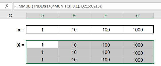
The ones vector j={1;1;1…} and the ones matrix J={1,1;1,1} are very useful in linear algebra and array formulas. The image below shows an example using the MUNIT function to create the Identity matrix I, the ones vector j, and the ones matrix J.

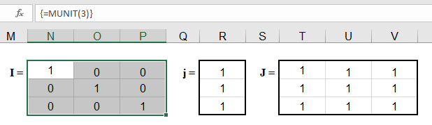
A simple way to create an n x n ones matrix (J) is to multiply the identity matrix by 0 and add 1, like this:

{ =1+0*MUNIT(n) }

The ones vector (j) of size n x 1 can be created by using INDEX to return the first column of the ones matrix, like this:

{ =INDEX(1+0*MUNIT(n),0,1) }

In older versions of Excel that don’t support the MUNIT function, you can create the ones vector, ones matrix and identity matrix using these formulas:

j =(1+0*ROW(INDIRECT("1:"&n)))
J =IF(ISERROR(OFFSET(INDIRECT("A1"),0,0,n,n)),1,1)
I =IF( ROW(OFFSET(INDIRECT("A1"),0,0,n,n)) = COLUMN(OFFSET(INDIRECT("A1"),0,0,n,n)), 1, 0)

Repeating Rows or Columns to Create a Matrix

Sometimes you may need to form a matrix by repeating a row or column. This can be done using MMULT and the ones vector.

If you want to create a matrix with n rows by repeating row={1, 2, 3}, use the array formula =MMULT(j,row) where j is size n x 1.

{ =MMULT( INDEX(1+0*MUNIT(n),0,1), row) }

If you want to create a matrix with k columns by repeating col={1;2;3}, use the array formula =MMULT(col,TRANSPOSE(j)) where j is size k x 1.

{ =MMULT(col, TRANSPOSE(INDEX(1+0*MUNIT(k),0,1)) ) }

ROW or COLUMN Sums using the ONES Vector

It turns out that the ONES vector is very important in statistics for performing a very simple matrix operation: summing the rows or columns. Let’s say you have a range of size n (rows) x k (columns). You could either use the SUM function separately for each row or column, or you could use array formulas.

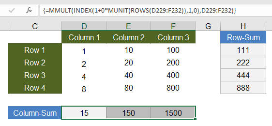
Column-Sum: To the sum the values within each COLUMN of the matrix and return the sums as a 1 x n array (or row vector), use

ones_vector =INDEX(1+0*MUNIT(ROWS(range)),0,1)
column_sum =MMULT(TRANSPOSE(ones_vector),range)

Row-Sum: To sum the values within each ROW of the matrix and return the sums as a k x 1 array (or column vector), use

ones_vector =INDEX(1+0*MUNIT(COLUMNS(range)),0,1)
row_sum =MMULT(range,ones_vector)

Creating a DIAGONAL Matrix

Element-wise multiplication of matrices can be used to create a Diagonal matrix. A Diagonal matrix is a special matrix where all of the off-diagonal terms are zeros. To create the Diagonal matrix, you multiply the matrix by the Identity matrix of the same size:

Diagonal =A*MUNIT(ROWS(A))

Many programs (but not Excel) include a function like diag(matrix) which returns an n x 1 vector containing the diagonal terms of an n x n matrix. To return the diagonal as a vector, you can use the row-sum operation on the Diagonal like this:

diag(A) =MMULT(A*MUNIT(ROWS(A)),(1+0*ROW(INDIRECT("1:"&ROWS(A)))))

Find the TRACE of a Square Matrix

The trace of a square matrix is just the sum of the diagonal elements. Therefore, the formula for calculating the trace is just:

trace(A) =SUM( A*MUNIT(ROWS(A)) )

Other Array Formula Examples

Linear Regression

The trend lines in an Excel chart allow you to do simple linear regression, but you can also do linear regression in Excel using matrix and array functions. It’s much easier to just use the LINEST function, but for fun I give the general formula for calculating the b matrix (the least squares estimators) when you have the y and X matrix. Or in other words, if you want to solve for b starting from y=Xb, you can do that using the formula b=(X‘X)^-1X‘y which in Excel is:

{ =MMULT(MMULT(MINVERSE(MMULT(TRANSPOSE(x),x)),TRANSPOSE(x)),y) }

Alternate XNPV Function

If for some reason you don’t like Excel’s XNPV function or for some reason you need to use 360 days in a year instead of 365, you can use the following array formula in place of XNPV, where r is the discount rate.

{ =SUM(values_range/((1+r)^((date_range-INDEX(date_range,1))/365))) }

Running XIRR Formula

My Investment Tracker calculates an annualized compounded rate of return using a running XIRR array formula.

Some References for Array Formulas in Excel

Guidelines and Examples of Array Formulas at support.office.com
Array Formulas at cpearson.com — Some detailed information about using array formulas in Excel, along with some example array functions.
Matrix Functions in Excel at bettersolutions.com — Examples showing the use of MDETERM, MINVERSE, MMULT, and TRANSPOSE.
Using Excel to find Eigenvalues and Eigenvectors
A.C.Rencher, Methods of Multivariate Analysis, John Wiley & Sons, Inc.: New York, 1995.

Источник

Excel is among the most powerful and widely used spreadsheet tools which eases organizing numbers and data within the sheets with pre-built formulas and functions. In this article, we are going to study Array Formulas. Arrays are one of them. Using Excel Array Formulas, make it super easy to handle a lot of data. Before understanding and using the Array formulas, let’s first understand what is Array in Excel?

Array in Excel

An Array in Excel is the structure that holds a collection of data. These data can be in the form of numbers or texts. There could be an array of 1-D or 2-D as well in Excel. For example, the array of fruits in excel would be written something like this:-

{“Apple”, “Banana”, “Grapes”, “Guava”}

We can directly enter it into the sheet by selecting the cells where you want to enter the data and then writing the array preceded by an “=” sign. After these press Ctrl+Shift+Enter. For example, let’s enter these values in cells A1 to D1.

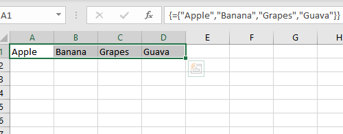
The array created here is a horizontal array. You can also create a vertical array by changing the selected cells. You can create an array by specifying the starting and the ending positions, for example, if you wish to make an array of elements between A1 to F1 then you can write A1:F1. Now. let’s move to array formulas.

Array formulas

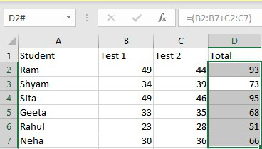
Array formulas enable to process of several values and give several outputs. In a simple world, it can do multiple calculations and reduce a lot of human efforts. In other words, we can say that it solves array calculations and give an array as output too. Let’s understand more of them with an example, of students with their test marks,

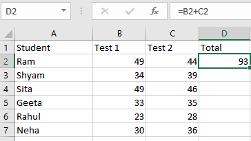
Here, we have used a formula to evaluate the result in the ‘Total’ field. For inserting the formula, click on the cell where you want to store the answer and write the formula. Now, let’s try to calculate the same for all students

For calculating the total for all the students, select the field where you want to store them, now select the range, and insert the formula. Array formulas are available in every version of Excel, so you don’t worry about your excel version. There are hundreds of operations possible using array formulas, which we will discuss in this article later. But before proceeding let’s understand what is the need to use an array formula.

Why use an Array Formula?

Array formulas are to most powerful yet most easy-to-use calculation tools which could be used to perform complex calculations and take place of hundreds of formulas with a single formula. You can further specify conditions for the calculation of data. Not just calculations you can also count the chars in cells, add date, day, or time, and even pick random data.

How to insert an Array Formula?

Before entering the Array formula fir of all we understand some important points about the Array formula:

After typing the formula you have to press keys CTRL+SHIFT+ENTER together. It will automatically change the normal formula into an array formula.
If you manually type braces around the formula then it will not convert the formula into an array formula. You have to use CTRL+SHIFT+ENTER keys to convert the formula into an array formula.
Whenever you edit the array formula the braces will disappear automatically and you have to again press the combination of CTRL+SHIFT+ENTER keys.
If you forget to press the CTRL+SHIFT+ENTER keys then your formula will work as the normal formula.

Now let’s understand inserting an array formula.

Single Cell Array formula

Every array formula returns the result in either single or in multiple cells. So when an array formula returns its result in the single-cell then such type of formula is known as a single-cell array formula. Such types of formulas are SUM, AVERAGE, AGGREGATE, MAX, MIN, etc. Follow the following steps to use the single-cell array formula:

Step 1: Select the cell where you want to store the answer.

Step 2: Now go to the formula bar and write an “=” sign.

Step 3: Now to formulas (highlighted below), and select the operation you want to perform.

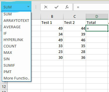
Step 4: Here we want to perform the sum operation. Click on sum and a new popup will open. Write the cells you want to perform the operation with.

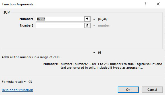
Multi-Cell Array Formula

If you wish to perform the same calculation with more cells then you can use the multi-cell formula. You can implement it in two ways. Functions like TRANSPOSE, TREND, FREQUENCY, LINEST, etc are used for the multi-cell arrays. Implement the formula in single-cell by following the above steps. Now, drag the selection up to the cells you want to implement the formula. Below is the implementation of doing that.

Alternatively,

Specify the range of cells and an operator between them. For example, =(B1:B7 + C2:C7) and press Ctrl+Shift+Enter.

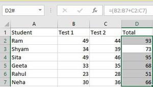
Excel Array Constants

Excel array contacts are a set of static values and can’t be changed. These values remain constant regardless of the operations performed on them. Now we will see how to create Array Constants in Excel and will perform different actions on them. There are three types of array constant available:

1. Horizontal or Row Array constant

A horizontal constant is present in a row. To create a horizontal constant we have to type multiple values separated by a comma in the enclosed braces. To enter a row array follow these steps below:

Step 1: Select the cells you want to work with.

Step 2: Go to the formula bar and start with an equal sign.

Step 3: Now enter the array you want to create in braces {}, separated by commas(,). Ex:- ={1,2,3,4,5}

Step 4: Now press Ctrl+Shift+Enter.

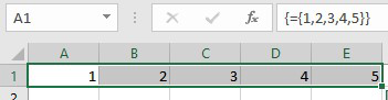
2. Vertical or Column Array

Vertical array constants are generally present in Column Array. To create a vertical constant we have to type multiple values separated by a semicolon in the enclosed braces. To enter a column array follow these steps below:

Step 1: Select the cells you want to work with.

step 2: Go to the formula bar and start with an equal sign.

Step 3: Now enter the array you want to create in braces {} separated with termination sign(;). Ex:- ={“Coding”;”GFG”;”GeeksforGeeks”}

Step 4: Now press Ctrl+Shift+Enter.

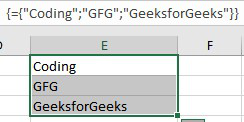
3. 2-D array

In Excel, you are allowed to create a 2-D array. So to create a 2-D array constant, we have to type multiple values in which rows are separated by semicolons and d columns are separated by commas. Let’s understand the implementation of a 2-d array.

Step 1: Select the cells you want to work with.

Step 2: Go to the formula bar and start with an equal sign.

Step 3: Now enter the array you want to create in braces {} separated with commas(,) for entering the values in same row, termination sign(;) for row change. Ex:- ={1,2,3;”Coding”,”GFG”,”GeeksforGeeks”}

Step 4: Now press Ctrl+Shift+Enter.

Working with Constant arrays

In the Excel formula, array constants are the important part. Some of the important concepts of Array constant are:

1. Elements: To create elements of array constant we have to follow the following points:

The elements of an array constant must be of numeric, alphabetic, boolean, or scientific notation and each of them is separated by commas or semicolons.
The elements of an array constant do not contain an array, cell reference, dates functions formulas, defined names, etc.
You can also be allowed to use text in the array of the element but the text is surrounded by hyphens(“”).

2. Naming Array Constants: You can name any array and use them as a variable for further references. For naming an array, follow the steps below:

Go to the formula tab. and select Define Name.
Write the array name in the name. You can also add some comments related to your array.
Click on OK.

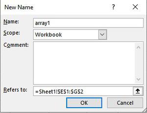
3. Common Errors: Following are the common errors that will happen while working with array constants:

The use of delimiters in between the elements.
The selection of range is also an important point to remember.

Unary Operator in Excel Array Formulas

Using unary operators we can process the array using AND and OR operators.

AND: It is denoted by an asterisk(*) symbol. It returns true if and only if all conditions are true,
OR: It is denoted by a plus(+) symbol. It returns true if any of the statement is true.

These operators are more useful when you have the same variable with a different value. For example, let’s consider a case, where data of 3 sellers of different months are given and you have to how much Shyam sold potatoes.

Источник

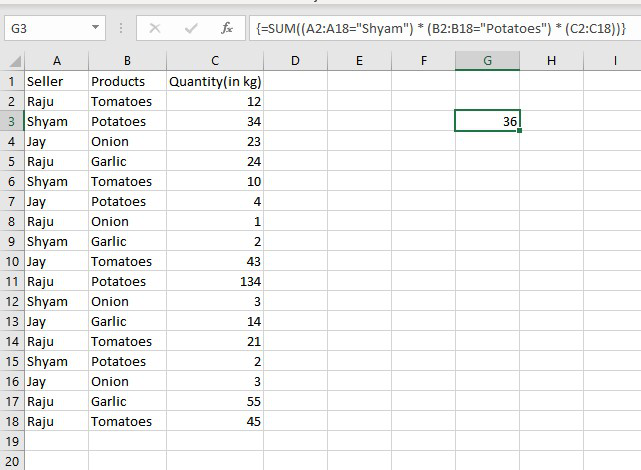
The COLUMNS function is a built-in function in Microsoft Excel. It falls under the category of LOOKUP functions in Excel. The COLUMNS function returns the total number of columns in the given array or collection of references. The purpose of the COLUMNS formula in Excel is to know the number of columns in an array of references.

For example, the formula =COLUMNS(A1:E3) will return as 5 since the range A1:E3 has 5 columns, A, B, C, D, and E, respectively.

What Is COLUMNS Function In Excel?
- Syntax
- How To Use COLUMNS Formula In Excel?
- Examples
- Important Things To Note
- Frequently Asked Questions
- Columns Function in Excel Video
- Recommended Articles

The COLUMNS function in excel is used to find the number of columns used in the worksheet.
The formula of the columns function in excel is =COLUMN(array), where the array is the only mandatory argument.
The array shows the range of cells for which the number of columns is derived.
We can choose either a single cell or a range as the value in the array argument.
It is important to know that the function will return only the number of columns even if the chosen array has multiple rows and columns.

Syntax

array = This is a required parameter. An array / a formula resulting in an array / a reference to a range of Excel cells for which the number of columns is to be calculated.

The COLUMNS function has only one argument, and it is mandatory.

How To Use COLUMNS Formula In Excel?

You can download this COLUMNS Function Excel Template here – COLUMNS Function Excel Template

The said function is a worksheet (WS) function. As a WS function, columns can be inserted as a part of the formula in a worksheet cell.

Let us look at the examples given below to understand the use of the COLUMNS function in excel.

Examples

Example #1 – Total Columns In A Range

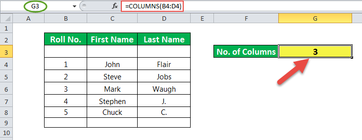
In the example of this column, cell G3 has a formula associated with it. So, G3 is a result cell.

The argument for the COLUMNS function in excel is a cell range, which is B4:D4. Here, B4 is a starting cell, and D4 is the ending cell.

The number of columns between these two cells is 3. So, the result is 3.

Example #2 – Total Cells In A Range

In this example, cell G4 has a formula associated with it. So, G4 is a result cell.

The formula is COLUMNS (B4: E8) * ROWS*B4: E8). Then, multiplication is performed between the total number of columns and a total number of rows for the given range of cells in the sheet.

Here, the total number of columns is four, and the total number of rows is 5. So, the total number of cells is 4*5 = 20.

Example #3 – Get The Address Of The First Cell In A Range

Here, the dataset is named data. Further, this data is used in the formula.

You may refer to the steps given below to name the dataset.

Step 1: Select the cells.
Step 2: Right-click and choose Define Name.
Step 3: Name the dataset as data.

In the example of these columns, cell G6 has a formula associated with it. So, G6 is a result cell. The formula is to calculate the first cell in the dataset represented by the name data. The result is $B$4, i.e., B4, the last cell in the selected dataset.

The formula uses the ADDRESSES function, which has two parameters: row number and column number.

E.g., ADDRESS (8,5) returns $B$4. Here, 4 is the row number, and 2 is the column number. So, the function returns a cell denoted by these row and column numbers.

Here, a row number is calculated by

ROW(data)

And the column number is calculated by

COLUMN(data)

Example 4 – Get The Address Of The Last Cell In A Range

Here, the dataset is named data. Further, this data is used in the column’s formula in Excel. We can refer to the steps given below to name the dataset.

Step 1: Select the cells.
Step 2: Right-click and choose Define Name.
Step 3: Name the dataset as data.

In this COLUMNS example, cell G5 has a formula associated with it. So, G5 is a result cell. The formula is to calculate the last cell in the dataset represented by the name data. The result is $E$8, i.e., E8, the last cell in the selected dataset.

The formula uses the ADDRESSES function, which has two parameters: row number and column number.

E.g., ADDRESS (8,5) returns $E$8. Here, 8 is the row number, and 5 is the column number. So, the function returns a cell denoted by these row and column numbers.

Here, the row number is calculated by

ROW(data)+ROWS(data-1)

And the column number is calculated by

COLUMN(data)+COLUMNS(data-1)

Important Things To Note

The argument of the COLUMNS function in Excel can be a single cell address or a range of cells.
The argument of the COLUMNS function cannot point to multiple references or cell addresses.

Frequently Asked Questions

1) What is the columns function in excel?

Columns Function in excel is a built-in excel function used to derive the number of columns used in the worksheet. The syntax of the COLUMNS function in excel is =COLUMNS(array). For example, consider the table with details of 3 employees.

We can calculate the number of columns used in the data using the columns function in excel.

Step 2: Select the range A1:C4 as shown in the below image.

Step 3: Press Enter key
We will get the result as shown in the below image.

2) When can we use the columns function in excel?

Columns Function in excel is used when we have to find the number of columns used in the data. Especially while working with large datasets, this function will be useful.

3) How to insert columns function in excel?

We can insert columns function in excel by selecting Formulas > Lookup & Reference in the Function Library group > COLUMNS function.

Alternatively, we can also type =COLUMNS and choose the cell array.

Columns Function in Excel Video

Example

In the example above, the three ranges map to arrays in a «row by column» scheme like this:

B5:D5 // 1 row x 3 columns
B8:B10 // 3 rows x 1 column
B13:D14  // 2 rows x 3 columns

If we display the values in these ranges as arrays, we have:

B5:D5={"red","green","blue"}
B8:B10={"red";"green";"blue"} 
B13:D14={10,20,30;40,50,60}

Notice arrays must represent a rectangular structure.

Array syntax

All arrays in Excel are wrapped in curly brackets {} and the delimiters between array elements indicate rows and/or columns. In the US version of Excel, a comma (,) separates columns and a semicolon (;) separates rows. For example, both arrays below contain numbers 1-3, but one is horizontal and one is vertical:

{1,2,3} // columns (horizontal)
{1;2;3} // rows (vertical)

Text values in an array appear in double quotes («») like this:

{"a","b","c"}

To «see» the array associated with a range, start a formula with an equal sign (=) and select the range. Then use the F9 key to inspect the underlying array. You can also use the ARRAYTOTEXT function to show how columns and rows are represented. Set format to 1 (strict) to see the complete array.

Delimiters in other languages

In other language versions of Excel, the delimiters for rows and column can vary. For example, the Spanish version of Excel uses a backslash () for columns and a semicolon (;) for rows:

{123} // columns
{1;2;3} // rows

Arrays in formulas

Since arrays map directly to ranges, all formulas work with arrays in some way, though it isn’t always obvious. A simple example is a formula that uses the SUM function to sum the range A1:A5, which contains 10,15,20,25,30. Inside SUM, the range resolves to an array of values. SUM then sums all values in the array and returns a single result of 100:

=SUM(A1:A5)
=SUM({10;15;20;25;30})
=100

Note: you can use the F9 key to «see» arrays in your Excel formulas. See this video for a demo on using F9 to debug.

Array formulas

Array formulas involve an operation that delivers an array of results. For example, here is a simple array formula that returns the total count of characters in the range A1:A5:

=SUM(LEN(A1:A5))

Inside the LEN function, A1:A5 is expanded to an array of values. The LEN function then generates a character count for each value and returns an array of 5 results. The SUM function then returns the sum of all items in the array.

Dynamic arrays

With the introduction of Dynamic Array formulas in Excel, arrays have become more important, since it is easier than ever to write formulas that work with multiple results at the same time.

Источник

Author: Oscar Cronquist Article last updated on July 22, 2022

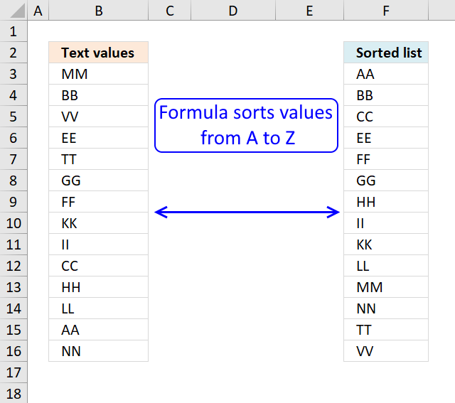
Table of Contents

Sort a column — Excel 365
Sort a column using array formula
Two columns sorting by the second column — Excel 365
Two columns sorting by the second column
Sort alphanumeric values

1. Sort a column — Excel 365

Excel 365 formula in cell D3:

=SORT(B3:B16)

The SORT function sorts values from a cell range or array

Function syntax: SORT(array,[sort_index],[sort_order],[by_col])

2. Sort a column using array formula

I am inspired once again by the article Sorting Text in Excel using Formulas at Pointy haired Dilbert. In Chandoo´s article, he sorts text with a «helper» column. My goal with this article is to show you how to sort text cells alphabetically without a helper column.

Here is an example, cell range $A$2:$A$15 contains text values.

Here is how to automatically sort text cells without any user interaction in cell B2:

Array formula in cell B2:

=INDEX($A$2:$A$15, MATCH(SMALL(COUNTIF($A$2:$A$15, «<«&$A$2:$A$15), ROW(1:1)), COUNTIF($A$2:$A$15, «<«&$A$2:$A$15), 0))

This article demonstrates how to filter a unique distinct list sorted from A to Z:

Recommended articles

test

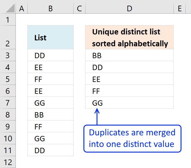
The following post shows you how to sort and filter duplicate values alphabetically:

Recommended articles

test

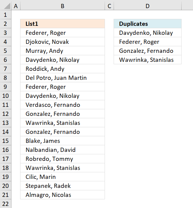
Learn how to sort a multi-column cell range alphabetically and display the values in a single column:

Recommended articles

Sort a data set using an array formula:

Recommended articles

test

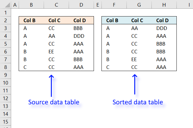
Tip! You can sort a data set in any way you like it, if you convert it to an excel defined table: Excel table — Sort data

How to create an array formula

Copy (Ctrl + c) and paste (Ctrl + v) array formula into formula bar.
Press and hold Ctrl + Shift.
Press Enter once.
Release all keys.

Copy cell B2 and paste it down as far as needed.

Recommended articles

test

Explaining array formula in cell B2

=INDEX($A$2:$A$15, MATCH(SMALL(COUNTIF($A$2:$A$15, «<«&$A$2:$A$15), ROW(1:1)), COUNTIF($A$2:$A$15, «<«&$A$2:$A$15), 0))

Step 1 — Count «smaller» values

COUNTIF(range,criteria) counts the number of cells within a range that meet the given condition

=INDEX($A$2:$A$15, MATCH(SMALL(COUNTIF($A$2:$A$15, «<«&$A$2:$A$15), ROW(1:1)), COUNTIF($A$2:$A$15, «<«&$A$2:$A$15), 0))

COUNTIF($A$2:$A$15, «<«&$A$2:$A$15)

becomes

COUNTIF({MM,BB,VV,EE,TT,GG,FF,KK,KK,II,CC,HH,LL,AA,NN}, «<«&MM,»<«&BB,»<«&VV,»<«&EE,»<«&TT,»<«&GG,»<«&FF,»<«&KK,»<«&II,»<«&CC,»<«&HH,»<«&LL,»<«&AA,»<«&NN)

The first value in this array formula is «MM». Let´s see what happens when COUNTIF calculates how many values is small than «MM».

COUNTIF({MM,BB,VV,EE,TT,GG,FF,KK,II,CC,HH,LL,AA,NN}, «<«&»MM»

becomes

COUNTIF({MM»<«&»MM»,BB»<«&»MM»,VV»<«&»MM»,EE»<«&»MM»,TT»<«&»MM»,GG»<«&»MM»,FF»<«&»MM»,KK»<«&»MM»,II»<«&»MM»,CC»<«&»MM»,HH»<«&»MM»,LL»<«&»MM»,AA»<«&»MM»,NN»<«&»MM»}

MM<MM is FALSE and BB<MM is TRUE and so on.. The array becomes:

COUNTIF({FALSE, TRUE, FALSE, TRUE, FALSE, TRUE, TRUE, TRUE, TRUE, TRUE, TRUE, TRUE, TRUE, FALSE}

becomes

COUNTIF({0, 1, 0, 1,0, 1 , 1 ,1 ,1 ,1 ,1 ,1 ,1 ,1 ,1 ,1 ,0} and the total is 10 which is the first number in the returning array. 0+1+0+1+0+1+1+1+1+1+1+1+1+1+1+1+0 = 10

Next is COUNTIF({MM,BB,VV,EE,TT,GG,FF,KK,II,CC,HH,LL,AA,NN}, «<«&»BB»)

becomes

COUNTIF({MM»<«&»BB»,BB»<«&»BB»,VV»<«&»BB»,EE»<«&»BB»,TT»<«&»BB»,GG»<«&»BB»,FF»<«&»BB»,KK»<«&»BB»,II»<«&»BB»,CC»<«&»BB»,HH»<«&»BB»,LL»<«&»BB»,AA»<«&»BB»,NN»<«&»BB»})

becomes

COUNTIF({FALSE, FALSE, FALSE, FALSE, FALSE, FALSE, FALSE, FALSE, FALSE, FALSE, FALSE,FALSE , TRUE, FALSE})

becomes

COUNTIF({0, 0, 0, 0,0, 0, 0,0,0,0,0,0,0,0,0,1,0}) and the total is 1 which is the second number in the returning array.

and so on…

COUNTIF($A$2:$A$15, «<«&$A$2:$A$15) returns this array:

{10, 1,13,3,12,5,4,8,7,2,6,9,0,11}

Recommended articles

test

Step 2 — Return the k-th smallest number in array

SMALL(array,k) returns the k-th smallest row number in this data set.

SMALL({10, 1,13,3,12,5,4,8,7,2,6,9,0,11}, ROW(1:1)) returns the smallest number in this data set, 0 (zero).

Recommended articles

test

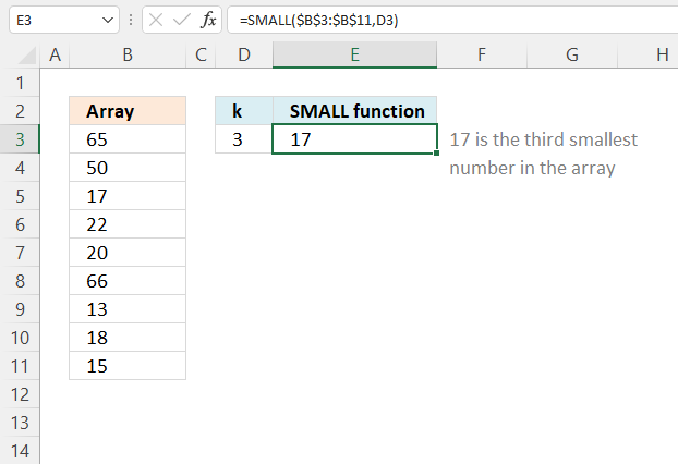
How to use the SMALL function
The SMALL function lets you extract a number in a cell range based on how small it is compared to the other numbers in the group.

Step 3 — Find position in array

MATCH(lookup_value;lookup_array; [match_type]) returns the relative position of an item in an array that matches a specified value

MATCH(SMALL(COUNTIF($A$2:$A$15, «<«&$A$2:$A$15), ROW(1:1)), COUNTIF($A$2:$A$15, «<«&$A$2:$A$15), 0)

becomes

MATCH(0, {10, 1,13,3,12,5,4,8,7,2,6,9,0,11}, 0) and returns 13.

Step 4 — Return value

INDEX(array,row_num,[column_num]) returns a value or reference of the cell at the intersection of a particular row and column, in a given range.

=INDEX($A$2:$A$15, MATCH(SMALL(COUNTIF($A$2:$A$15, «<«&$A$2:$A$15), ROW(1:1)), COUNTIF($A$2:$A$15, «<«&$A$2:$A$15), 0))

becomes

=INDEX($A$2:$A$15, 13) and returns AA in cell B2.

Get Excel sample file for this tutorial

Sorting-text-cells-using-array-formulas.xls
(Excel 97-2003 Workbook *.xls)

3. Sort two columns by the second column — Excel 365

4. Sort two columns by the second column

Array Formula in cell E2:

=INDEX($B$2:$B$9, MATCH(SMALL(COUNTIF($B$2:$B$9, «<«&$B$2:$B$9), ROW(1:1)), COUNTIF($B$2:$B$9, «<«&$B$2:$B$9), 0))

Array Formula in cell D2:

=INDEX($A$2:$A$9, SMALL(IF(E2=$B$2:$B$9, MATCH(ROW($B$2:$B$9), ROW($B$2:$B$9))), SUM(—(E2=$E$2:E2))))

Get excel *.xlsx

Two columns sorting by the second column.xlsx

Источник

A lesson on how to combine columns horizontally and how to stack columns vertically in Excel by SpreadsheetClass.com

There are a variety of different ways to combine columns in Excel, and I am going to show you five different formulas that you can use to combine multiple columns into one. Three of these formulas will combine columns horizontally, and two of them will combine columns vertically.

Directly below are quick instructions for combining columns, but also look further below for detailed examples, as well as additional ways of combining columns.

To combine columns horizontally in Excel, follow these steps:

Type an equals sign and then a column reference, such as =A3:A12 to specify the first column to combine
Type an ampersand (&)
Type the address of the other column that you want to combine with, such as B3:B12
Press enter on the keyboard. The full formula will look like this: =A3:A12&B3:B12 (If you are using an older version of Excel, you will need to hold «Ctrl» and «Shift» on the keyboard before pressing «Enter». If you do this, curly brackets will appear before and after your formula, like this: {=A3:A12&B3:B12}
Optional: If you want, you can add special characters between the combined columns by using additional ampersands, and any character that you want between quotation marks, like this =A3:A12&» «&B3:B12

(See detailed instructions below for how to add spaces or special characters between the columns)

To combine columns vertically in Excel, follow these steps:

Method 1: Enter the following formula in a blank cell / column, to combine columns vertically: =IF(A3<>»»,A3,INDIRECT(«B»&ROW()-COUNTIF(A$3:A$1000,»<>»)))
Method 2: Enter the following formula in a blank cell / column, to combine columns vertically while alternating between rows: =INDEX($A$2:$B$1000,ROW()/2,MOD(ROW(),2)+1)
Use the fill handle or copy and paste the formula downwards

Here are the formulas that will combine columns in Excel:

Horizontal column combination formulas

=A3:A12&» «&B3:B12 Legacy / CSE Version: {=A3:A12&» «&B3:B12}
=CONCAT(A3,» «,B3)
=CONCATENATE(A3:A12,» «,B3:B12) Legacy / CSE Version: {=CONCATENATE(A3:A12,» «,B3:B12)}

Vertical column combination formulas

=IF(A3<>»»,A3,INDIRECT(«B»&ROW()-COUNTIF(A$3:A$1000,»<>»)))
=INDEX($A$2:$B$1000,ROW()/2,MOD(ROW(),2)+1)

This lesson will teach you how to combine columns in Excel, but check out this article if you want to learn how to combine columns in Google Sheets.

Using arrays in Excel

Notice that some of the formulas we are using in this lesson use what are called «arrays». An array formula is entered into a single cell but applies the formula to a range of cells. If you are using an older version of Excel, when using «arrays», you will need to hold «Ctrl» and «Shift» on the keyboard, and then press «Enter» when entering your array formulas. This is called a CSE (Control / Shift / Enter) formula, and is also sometimes called a «Legacy» array, as opposed to newer «Dynamic» arrays that do not require this extra step.

After doing the Ctrl / Shift / Enter method, your formula will be wrapped in curly brackets { }. Notice that the two formulas below will perform the same task, but were simply entered differently, the bottom formula being the «CSE» formula.

=A3:A10&B3:B10

{=A3:A10&B3:B10}

Combine columns in Excel (Horizontal)

First I am going to show you how to combine columns in Excel horizontally.

If you have two columns that you would like to combine the contents of, where the values of the cells in each row are to be combined together horizontally, then there are a few simple ways of doing this:

The first method (using the «&» operator / ampersand), will allow you to not only combine/merge two columns horizontally, but will also allow you to separate the contents with specified values/ strings of text, and will also allow you to combine more than two columns if you wish
The second method (using the CONCATENATE function), will allow you to combine the contents of two or more columns horizontally. The CONCATENATE function is almost identical to CONCAT, and I will mention more about this function below.

Both of these methods can be used to combine individual cells, without having to use the ARRAYFORMULA function.

Using the AND operator / ampersand (&) to combine columns

First I will show you the most common and functional way of combining columns horizontally in Excel. In this example we will combine first and last names into a single column.

By using the «&» operator you will be able to combine multiple columns in Excel, and you will also be able to specify values and strings of text that you would like to attach to the column combination.

To combine the data from individual cells in Excel (Such as first & last name), follow these steps:

Type an equals sign, and then type the address for the first cell that you want to combine with, such as A3
Type an ampersand (&)
Type the address of the another cell that you want to combine with, such as B3
Press enter on the keyboard. The full formula will look like this: =A3&B3
Copy / fill down the formula to use it on the entire column, or turn the cell references into range references to turn the formula into an array

In this first example we have a list of first names in one column, and last names in another column… and we want to combine these columns horizontally so that in each row the full combined name is displayed as a single text string, in a single column.

We will also put a separating space between the contents that are combined in this example. This is accomplished by using quotation marks with a space between them i.e. (» «) in the array formula (shown below).

The task: Horizontally combine the «first name» column with the «size» column, and put a space between the contents… so that the full name is displayed in a single column.

(Where the contents of the cells in each row are combined into a single text string separated by a space)

The logic: Horizontally combine the contents of the cells in the range A3:A12, with the contents of the cells from the range B3:B12, and add a space between the text/contents from the combined columns

The formula: The formula below, is entered in the blue cell (D3), for this example

=A3:A12&» «&B3:B12

{=A3:A12&» «&B3:B12} (Legacy / CSE Version)

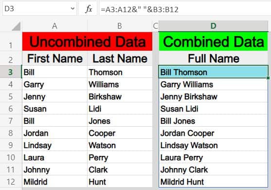
Remember to hold Ctrl + Shift + Enter to make an array formula, with older versions of Excel.

Combining more than 2 columns horizontally in Excel

If you want to combine more than 2 columns horizontally in Excel, you can do this with the «&» operator, which is also called an «ampersand».

For example, if you wanted to combine columns A, B and C, horizontally (with spaces between), then you could use the formula below.

=A3:A12&» «&B3:B12&» «&C3:C12

Using CONCAT or CONCATENATE to merge columns in Excel

In this example we are going to do the same thing as in the example above, but we are going to use different data. We have a list of clothing inventory items in one column, and the clothing size for that item listed in another column… and we want to combine these columns horizontally so that in each row the clothing item and size are displayed as a single text string, in a single column.

We will be using the CONCATENATE function, which is compatible with arrays, making it easy to combine an entire column with a single formula.

However, note that you can also use the CONCAT function to combine cells and even place spaces / characters between those columns, just like we did with the «&» symbol… but the CONCAT function does not work with arrays, and so if you use this to combine columns you will need to use one formula in each cell.

To combine the data from cells by using the CONCATENATE in Excel, follow these steps:

Type =CONCATENATE( to begin your formula
Type the address of the first cell that you want to combine with, such as A5
Type a comma, and then type the address of the next cell that you want to combine with, such as B5
Press enter on the keyboard. The full formula will look like this: =CONCATENATE(A5,B5)
Copy / fill down the formula to use it on the entire column, or change the cell references into range references to turn the formula into an array

To combine the data from cells with the CONCAT formula in Excel, follow these steps:

Type =CONCAT( to begin your formula
Type the address of the first cell that you want to combine with, such as A2
Type a comma, and then type the address of the next cell that you want to combine with, such as B2
Press enter on the keyboard. The full formula will look like this: =CONCAT(A3,B3)
Copy / fill down the formula to use it on the entire column

See the example / instructions above for how to add spaces / special characters between the columns.

The task: Horizontally combine the column that shows clothing items with the column that shows clothing sizes… so that the clothing item and size are displayed in a single column.

(Where the contents of the cells in each row are combined into a single text string)

The logic: Combine the range A3:B, and the range B3:B into a single column, so that the contents from the cells are horizontally merged into a single text string

The formula: The formula below, is entered in the blue cell (D3), for this example

=CONCATENATE(A3:A12,» «,B3:B12)

{=CONCATENATE(A3:A12,» «,B3:B12)} (Legacy / CSE Version)

The formulas above are the array version, but in the image you can see the basic version of the formula with one formula per cell.

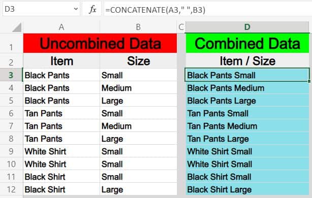
Notice that the CONCAT function (Shown Below) does the same thing as the CONCATENATE function (Shown Above)

=CONCAT(A3,» «,B3)

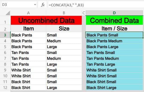
Now I am going to show you how to combine columns in Excel vertically, or in other words «stack columns».

There are 2 different ways to combine columns in Excel vertically by using formulas, depending on how you would like the formula to operate:

The first method (using the INDIRECT, ROW, and COUNTIF functions), will stack the column ranges that are specified on top of each other exactly as is
The second method (using the INDEX, ROW, and MOD functions with an array), will combine the contents from individual columns into a single column, but will alternate between columns for each row

Formula for combining (stacking) columns in Excel:

=IF(A3<>»»,A3,INDIRECT(«B»&ROW()-COUNTIF(A$3:A$99,»<>»)))

Formula for combining columns, while alternating back and forth between columns in Excel:

=INDEX($A$2:$B$99,ROW()/2,MOD(ROW(),2)+1)

* Note that both of these formulas must be copied / filled into the cells for the entire column (With one formula per cell).

Combining columns vertically while stacking one column on top of another column

In this example we have two different lists of inventory that we want to combine into one. Let’s say that two different employees counted clothing items in separate parts of your store, and that you want to combine the lists that they return to you into one list/column.

By using the INDIRECT function, the ROW function, and the COUNTIF function, we can create a formula that will stack the contents from one column, on top of the contents of another column. With the example / formula shown below, the contents of one entire column will be listed with the formula, before the contents of the second column are listed below it (As opposed to the alternating column method in the next example).

The task: Combine two lists of clothing items into a single list of unique inventory items… or in other words, make a single list that shows one of each item that is contained in inventory, by combining two lists

The logic: Combine the range A3:A10 and the range B3:B10 vertically into a single column

The formula: The formula below, is entered in the blue cell (D3), for this example

=IF(A3<>»»,A3,INDIRECT(«B»&ROW()-COUNTIF(A$3:A$1000,»<>»)))

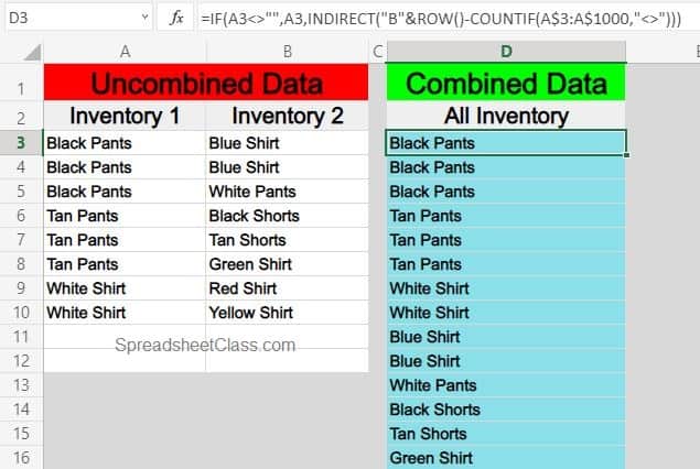
Make sure that you place your formula in the correct row, according to the beginning rows of the references in the formula (If the formula’s references begin at row 3, make sure that your first formula is in row 3.

Note in the example image how the formula in cell D3 has been copied into the cells below it. Remember to do this in your sheet as well.

Combining columns vertically while alternating from column to column for each row

In this example we are going to combine the same inventory lists from the previous example, vertically into a single column, but this time we are going to use a different formula that alternates between columns when listing the combined column data (As opposed to stacking one entire column on top of another entire column).

To do this we will use the INDEX function, the ROW function, and the MOD function.

The task: Combine two lists of clothing items into a single list, and show all items found

The logic: Combine the contents in range A3:A10 and the contents in range B3:B10 vertically into a single column

The formula: The formula below, is entered in the blue cell (D3), for this example

=INDEX($A$2:$B$1000,ROW()/2,MOD(ROW(),2)+1)

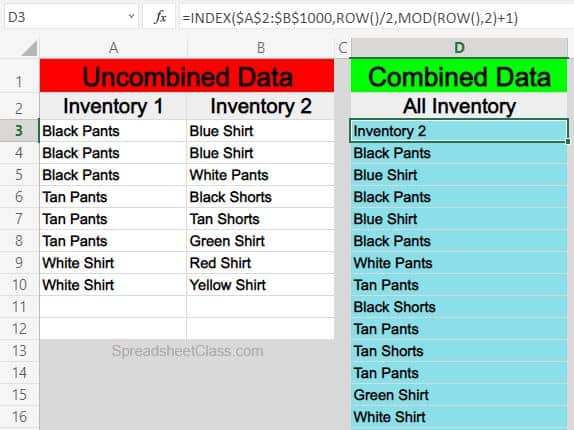
Like the formula in the previous example, make sure that your formula is placed in the correct row, according to the beginning rows of your formula references. However, with this particular formula, if your data begins on an odd row, such as row 3, your formula reference will need to begin on the previous / even row to make sure that all of the data is captured (As shown in the example image).

Note in the example image how the formula in cell D3 was copied into the cells below. Remember to do this in your sheet as well.

How to combine columns from separate sheets

You may find situations that require you to combine columns that are from separate tabs in Excel.

This can be done by simply referring to a certain tab name when specifying the ranges in the formula. So where you would normally set a range like «A1:C», when referencing another sheet while combining columns you will specify the tab name, by adding the tab name and an exclamation mark before listing the column and row for the range, like «TabName!A1:C»

However when the tab name has a space in it, you will need to use an apostrophe before and after typing the tab name, like ‘Tab Name’!A1:C.

Here is an example of how to combine columns from multiple tabs in Excel, where there are two lists in different tabs, to be combined into a single list on a completely separate tab.

Let’s say that you have a list of clothing items on one tab, another list of clothing items on a separate tab, and that you want to display a combined list of unique clothing items that are in inventory, on a completely different tab (meaning that there will be no duplicates).

*Note that you can reference specified tabs with any of the formulas that you learned in this article, but for this example we are using an array with the ampersand (&) to demonstrate how to combine columns from different tabs.

The task: Combine the list of clothing items on the tab labeled «List 1», with the list of clothing items on the tab labeled «List 2» and show a combined list of clothing items, on completely separate tab

The logic: Combine the range ‘List 1’!A3:A12, with the range ‘List 2’!A3:A12

The formula: The formula below, is entered in the blue cell (A3), for this example

=’List 1′!A3:A12&» «&’List 2′!B3:B12

Here are two different lists of clothing items, which are held on two separate tabs labeled, «List 1» and «List 2»

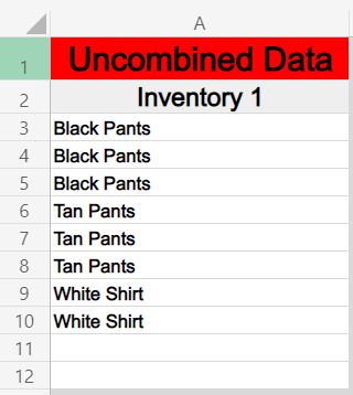
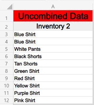
And here is a combined list of clothing items, where the formula and combined data are held on a separate tab

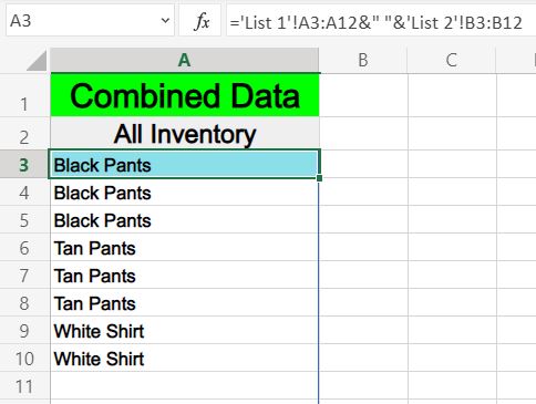
Pop Quiz: Test your knowledge

Answer the questions below about combining columns in Excel to refine your knowledge! Scroll to the very bottom to find the answers to the quiz.

Horizontal column combination formulas

=A3:A12&» «&B3:B12

=CONCAT(A3,» «,B3)

=CONCATENATE(A3:A12,» «,B3:B12)

Vertical column combination formulas

=IF(A3<>»»,A3,INDIRECT(«B»&ROW()-COUNTIF(A$3:A$1000,»<>»)))

=INDEX($A$2:$B$1000,ROW()/2,MOD(ROW(),2)+1)

Question #1

Which of the following formulas will allow you to combine columns vertically? (Select all that apply)

=A3:A100&» «&B3:B100
=CONCAT(A5,» «,B5)
=IF(A5<>»»,A5,INDIRECT(«B»&ROW()-COUNTIF(A$5:A$1000,»<>»)))
=CONCATENATE(A3:A100,» «,B3:B100)
=INDEX($A$5:$B$1000,ROW()/2,MOD(ROW(),2)+1)

Question #2

Which of the following formulas will put a space between the contents that are horizontally combined?

=CONCATENATE(A3:A100,B3:B100)
=A3:A100&» «&B3:B100

Question #3

True or False: For older versions of Excel, you must hold Ctrl + Shift + Enter on the keyboard before entering an array formula

True
False

Question #4

Which of the following formulas will combine columns horizontally?

=IF(A5<>»»,A5,INDIRECT(«B»&ROW()-COUNTIF(A$5:A$1000,»<>»)))
=CONCATENATE(A3:A100,» «,B3:B100)

Question #5

Which of the following formulas will stack / combine columns WITHOUT alternating between columns

=IF(A5<>»»,A5,INDIRECT(«B»&ROW()-COUNTIF(A$5:A$1000,»<>»)))
=INDEX($A$5:$B$1000,ROW()/2,MOD(ROW(),2)+1)

Answers to the questions above:

Question 1: 3, 5

Question 2: 2

Question 3: 1

Question 4: 2

Question 5: 1

Источник

Download our examples

Acknowledgement

Need more help?

See Also

Topics and Examples in This Article:

Watch the Intro Video

Entering and Identifying an Array Formula

Using Array Constants in Formulas

A Simple Array Formula Example

Entering a Multi-Cell Array Formula

Nested IF Array Formulas

MAX-IF Array Formula

LARGE-IF Array Formula

SMALL-IF Array Formula

SUM-IF Array Formula

COUNTIF Alternative: SUM-Boolean Array Formulas

SUM-ISERROR: Count the number of Error values in a range

SUM-ISBLANK: Count the number of Blank values in a range

SUM-NOT-ISBLANK: Count the number of Non-Blank values in a range

Multi-Criteria Boolean Array Formulas

SUM-IF Between Two Dates

Overlapping OR Conditions

Sequential Number Arrays

Variant #1: Create a Sequence of Whole Numbers from i to j

Variant #2: Create an n x 1 Vector of Whole Numbers Starting From s

Variant #3: Sequence of Dates Between START and END (inclusive)

Variant #4: Create an n x 1 Vector of Sequential Powers of 10

Formulas for Matrices

Element-Wise Multiplication of 2 Matrices

Creating the ONES Vector and ONES Matrix

Repeating Rows or Columns to Create a Matrix

ROW or COLUMN Sums using the ONES Vector

Creating a DIAGONAL Matrix

Find the TRACE of a Square Matrix

Other Array Formula Examples

Linear Regression

Alternate XNPV Function

Running XIRR Formula

Some References for Array Formulas in Excel

Array in Excel

Array formulas

How to insert an Array Formula?

Multi-Cell Array Formula

Excel Array Constants

Working with Constant arrays

Unary Operator in Excel Array Formulas

Table of Contents

Syntax

How To Use COLUMNS Formula In Excel?

Examples

Example #1 – Total Columns In A Range

Example #2 – Total Cells In A Range

Example #3 – Get The Address Of The First Cell In A Range

Example 4 – Get The Address Of The Last Cell In A Range

Important Things To Note

Frequently Asked Questions

Columns Function in Excel Video

Recommended Articles

Example

Array syntax

Delimiters in other languages

Arrays in formulas

Array formulas

Dynamic arrays

1. Sort a column — Excel 365

2. Sort a column using array formula

How to create an array formula

Explaining array formula in cell B2

Step 1 — Count «smaller» values

Step 2 — Return the k-th smallest number in array

Step 3 — Find position in array

Step 4 — Return value

Get Excel sample file for this tutorial

3. Sort two columns by the second column — Excel 365

4. Sort two columns by the second column

Get excel *.xlsx

Here are the formulas that will combine columns in Excel:

Horizontal column combination formulas

Vertical column combination formulas

Using arrays in Excel