
Содержание
- Columns and rows are labeled numerically in Excel
- Symptoms
- Cause
- Resolution
- More information
- A1 Reference Style vs. R1C1 Reference Style
- The A1 Reference Style
- The R1C1 Reference Style
- References
- Define and use names in formulas
- Name a cell
- Define names from a selected range
- Use names in formulas
- Manage names in your workbook with Name Manager
- Name a cell
- Define names from a selected range
- Use names in formulas
- Manage names in your workbook with Name Manager
- Need more help?
- How to change the name of the column headers in Excel
- How to get the current column name in Excel?
- 17 Answers 17
- How to sort in Excel by row, column names and in custom order
- Sort by several columns
- Sort in Excel by row and by column names
- Sort data in custom order (using a custom list)
- Sort data by your own custom list
Columns and rows are labeled numerically in Excel
Symptoms
Your column labels are numeric rather than alphabetic. For example, instead of seeing A, B, and C at the top of your worksheet columns, you see 1, 2, 3, and so on.
Cause
This behavior occurs when the R1C1 reference style check box is selected in the Options dialog box.
Resolution
To change this behavior, follow these steps:
- Start Microsoft Excel.
- On the Tools menu, click Options.
- Click the Formulas tab.
- Under Working with formulas, click to clear the R1C1 reference style check box (upper-left corner), and then click OK.
If you select the R1C1 reference style check box, Excel changes the reference style of both row and column headings, and cell references from the A1 style to the R1C1 style.
More information
A1 Reference Style vs. R1C1 Reference Style
The A1 Reference Style
By default, Excel uses the A1 reference style, which refers to columns as letters (A through IV, for a total of 256 columns), and refers to rows as numbers (1 through 65,536). These letters and numbers are called row and column headings. To refer to a cell, type the column letter followed by the row number. For example, D50 refers to the cell at the intersection of column D and row 50. To refer to a range of cells, type the reference for the cell that is in the upper-left corner of the range, type a colon (:), and then type the reference to the cell that is in the lower-right corner of the range.
The R1C1 Reference Style
Excel can also use the R1C1 reference style, in which both the rows and the columns on the worksheet are numbered. The R1C1 reference style is useful if you want to compute row and column positions in macros. In the R1C1 style, Excel indicates the location of a cell with an «R» followed by a row number and a «C» followed by a column number.
References
For more information about this topic, click Microsoft Excel Help on the Help menu, type about cell and range references in the Office Assistant or the Answer Wizard, and then click Search to view the topic.
Источник
Define and use names in formulas
By using names, you can make your formulas much easier to understand and maintain. You can define a name for a cell range, function, constant, or table. Once you adopt the practice of using names in your workbook, you can easily update, audit, and manage these names.

Name a cell
In the Name Box, type a name.
To reference this value in another table, type th equal sign (=) and the Name, then select Enter.
Define names from a selected range
Select the range you want to name, including the row or column labels.
Select Formulas > Create from Selection.
In the Create Names from Selection dialog box, designate the location that contains the labels by selecting the Top row, Left column, Bottom row, or Right column check box.
Excel names the cells based on the labels in the range you designated.
Use names in formulas
Select a cell and enter a formula.
Place the cursor where you want to use the name in that formula.
Type the first letter of the name, and select the name from the list that appears.
Or, select Formulas > Use in Formula and select the name you want to use.
Manage names in your workbook with Name Manager
On the ribbon, go to Formulas > Name Manager. You can then create, edit, delete, and find all the names used in the workbook.
Name a cell
In the Name Box, type a name.
Define names from a selected range
Select the range you want to name, including the row or column labels.
Select Formulas > Create from Selection.
In the Create Names from Selection dialog box, designate the location that contains the labels by selecting the Top row, Left column, Bottom row, or Right column check box.
Excel names the cells based on the labels in the range you designated.
Use names in formulas
Select a cell and enter a formula.
Place the cursor where you want to use the name in that formula.
Type the first letter of the name, and select the name from the list that appears.
Or, select Formulas > Use in Formula and select the name you want to use.
Manage names in your workbook with Name Manager
On the Ribbon, go to Formulas > Defined Names > Name Manager. You can then create, edit, delete, and find all the names used in the workbook.
In Excel for the web, you can use the named ranges you’ve defined in Excel for Windows or Mac. Select a name from the Name Box to go to the range’s location, or use the Named Range in a formula.
For now, creating a new Named Range in Excel for the web is not available.
Need more help?
You can always ask an expert in the Excel Tech Community or get support in the Answers community.
Источник
How to change the name of the column headers in Excel
In Microsoft Excel, the column headers are named A, B, C, and so on by default. Some users want to change the names of the column headers to something more meaningful. Unfortunately, Excel does not allow the header names to be changed.
The same applies to row names in Excel. You cannot change the row names, or numbering, but you can add your desired row names in column A for the corresponding rows.
Instead, if you want to have meaningful column header names, you can do the following.
- Click in the first row of the worksheet and insert a new row above that first row.
- How to add or remove a cell, column, or row in Excel.
- In the inserted row, enter the preferred name for each column.
- To make the row of column names more noticeable, you could increase the text size, make the text bold, or add background color to the cells in that row.
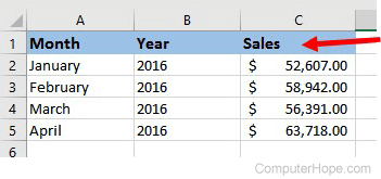
After inserting the new row and adding column header names, if you want to hide the default column header names, follow the steps below to hide column and row headers.
- In Microsoft Excel, click the File tab or the Office button in the upper-left corner.
- In the left navigation pane, click Options.
- In the Excel Options window, click the Advanced option in the left navigation pane.
- Scroll down to the Display options for this worksheet section. Uncheck the box for Show row and column headers.
The column and row headers are now hidden. To display them again, re-check the box in step 4 above.
Источник
How to get the current column name in Excel?
What is the function to get the current line number and the current column name for a cell in Excel?
17 Answers 17
You can use the ROW and COLUMN functions to do this. If you omit the argument for those formulas, the current cell is used. These can be directly used with the OFFSET function, or any other function where you can specify both the row and column as numerical values.
For example, if you enter =ROW() in cell D8, the value returned is 8. If you enter =COLUMN() in the same cell, the value returned is 4.
If you want the column letter, you can use the CHAR function. I do not recommend the use of letters to represent the column, as things get tricky when passing into double-letter column names (where just using numbers is more logical anyways).
Regardless, if you should still want to get the column letter, you can simply add 64 to the column number (64 being one character less then A ), so in the previous example, if you set the cell’s value to =CHAR(COLUMN()+64) , the value returned would be D . If you wanted a cell’s value to be the cell location itself, the complete formula would be =CHAR(COLUMN()+64) & ROW() .
Just an FYI, I got 64 from an ASCII table. You could also use the CODE formula, so the updated formula using this would be =CHAR(COLUMN() + CODE(«A») — 1) . You have to subtract 1 since the minimum value of COLUMN is always 1, and then the minimum return value of the entire formula would be B .
However, this will not work with two-letter columns. In that case, you need the following formula to properly parse two-letter columns:
Источник
How to sort in Excel by row, column names and in custom order
 by Alexander Frolov, updated on February 17, 2023
In this article I will show you how to sort Excel data by several columns, by column names in alphabetical order and by values in any row. Also, you will learn how to sort data in non-standard ways, when sorting alphabetically or numerically does not work.
I believe everyone knows how to sort by column alphabetically or in ascending / descending order. All you need to do is click the A-Z or Z-A buttons residing on the Home tab in the Editing group and on the Data tab in the Sort & Filter group:
However, the Excel Sort feature provides far more options and capabilities that are not so obvious but may come in extremely handy:
Sort by several columns
Now I’m going to show you how to sort Excel data by two or more columns. I will do this in Excel 2010 because I have this version installed on my computer. If you use another Excel version, you won’t have any problems with following the examples because the sorting features are pretty much the same in Excel 2007 and Excel 2013. You may only notice some differences in color schemes and dialogs’ layouts. Okay, let’s go ahead.
- Click the Sort button on the Data tab or Custom Sort on the Home tab to open the Sort dialog.
- Then click the Add Level button as many times as many columns you want to use for sorting:

From the «Sort by» and «Then by» dropdown lists, select the columns by which you want to sort your data. For example, you are planning your holiday and have a list of hotels provided by a travel agency. You want to sort them first by Region, then by Board basis and finally by Price, as shown in the screenshot:

- Firstly, the Region column is sorted first, in the alphabetic order.
- Secondly, the Board basis column is sorted, so that all-inclusive (AL) hotels are at the top of the list.
- Finally, the Price column is sorted, from smallest to largest.

Sorting data by multiple columns in Excel is pretty easy, isn’t it? However, the Sort dialog has plenty more features. Further on in this article I will show you how to sort by row, not column, and how to re-arrange data in your worksheet alphabetically based on column names. Also, you will learn how to sort your Excel data in non-standard ways, when sorting in alphabetical or numerical order does not work.
Tip. If values you wish to sort include text and numeric characters, check out How to sort mixed numbers and text in Excel.
Sort in Excel by row and by column names
I guess in 90% of cases when you are sorting data in Excel, you sort by values in one or several columns. However, sometimes we have non-trivial data sets and we do need to sort by row (horizontally), i.e. rearrange the order of columns from left to right based on column headers or values in a particular row.
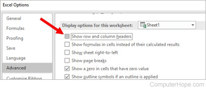
For example, you have a list of photo cameras provided by a local seller or downloaded from the Internet. The list contains different features, specifications and prices like this:
What you need is to sort the photo cameras by some parameters that matter the most for you. As an example, let’s sort them by model name first.
- Select the range of data you want to sort. If you want to re-arrange all the columns, you can simply select any cell within your range. We cannot do this for our data because Column A lists different features and we want it to stick in place. So, our selection starts with cell B1:

Click the Sort button on the Data tab to open the Sort dialog. Notice the «My data has headers» checkbox in the upper-right part of the dialog, you should uncheck it if your worksheet does not have headers. Since our sheet has headers, we leave the tick and click the Options button.

In the opening Sort Options dialog under Orientation, choose Sort left to right, and click OK.

Then select the row by which you want to sort. In our example, we select Row 1 that contains the photo camera names. Make sure you have «Values» selected under Sort on and «A to Z» under Order, then click OK.
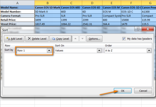
The result of your sorting should look similar to this:

I know that sorting by column names has very little practical sense in our case and we did it for demonstration purposes only so that you can get a feel of how it works. In a similar way, you can sort the list of cameras by size, or imaging sensor, or sensor type, or any other feature that is most critical for you. For instance, let’s sort them by price for a start.
What you do is go through steps 1 — 3 as described above and then, on step 4, instead of Row 2 you select Row 4 that lists retail prices. The result of sorting will look like this:
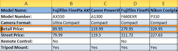
Please note that it’s not just one row that has been sorted. The entire columns were moved so that the data was not distorted. In other words, what you see in the screenshot above is the list of photo cameras sorted from cheapest to most expensive.
Hope now you’ve gained an insight into how sorting a row works in Excel. But what if we have data that does not sort well alphabetically or numerically?
Sort data in custom order (using a custom list)
If you want to sort your data in some custom order other than alphabetical, you can use the built-in Excel custom lists or create your own. With built-in custom lists, you can sort by days of the week or months of the year. Microsoft Excel provides two types of such custom lists — with abbreviated and full names:
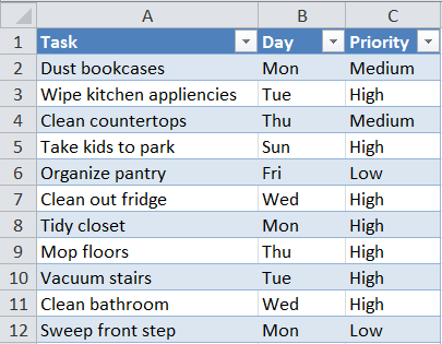
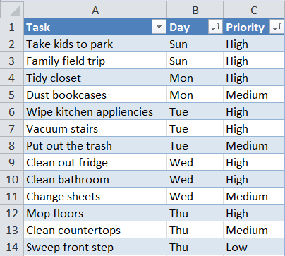
Say, we have a list of weekly household chores and we want to sort them by due day or priority.
- You start with selecting the data you want to sort and then opening the Sort dialog exactly like we did when sorting by multiple columns or by column names (Data tab >Sort button).
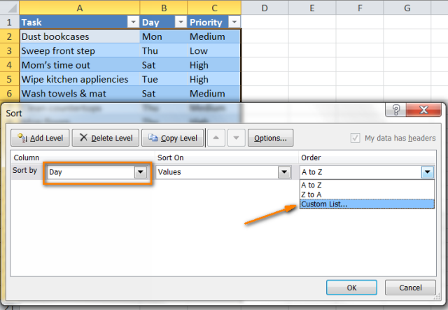
- In the Sort by box, select the column you want to sort by, in our case it is the Day column since we want to sort our tasks by the days of the week. Then choose Custom List under Order as shown in the screenshot:
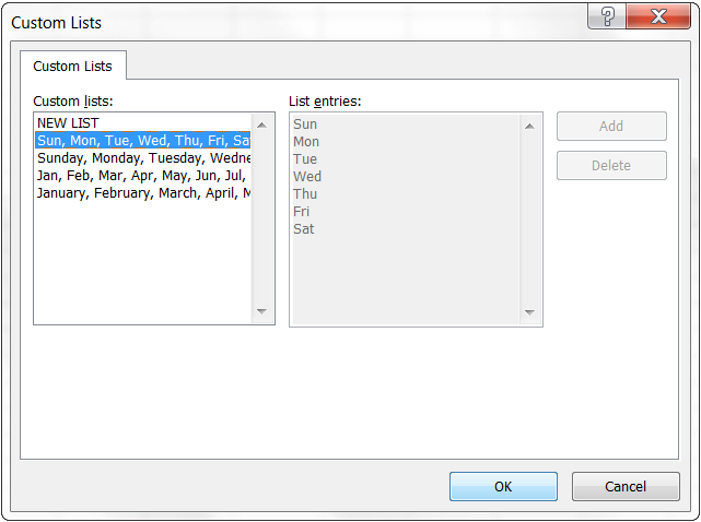
In the Custom Lists dialog box, select the needed list. Since we have the abbreviated day names in the Day columns, we choose the corresponding custom list and click OK.

That’s it! Now we have our household tasks sorted by the day of the week:

Note. If you want to change something in your data, please keep in mind that new or modified data won’t get sorted automatically. You need to click the Reapply button on the Data tab, in the Sort & Filter group:

Well, as you see sorting Excel data by custom list does not present any challenge either. The last thing that is left for us to do is to sort data by our own custom list.
Sort data by your own custom list
As you remember, we have one more column in the table, the Priority column. In order to sort your weekly chores from most important to less important, you proceed as follows.
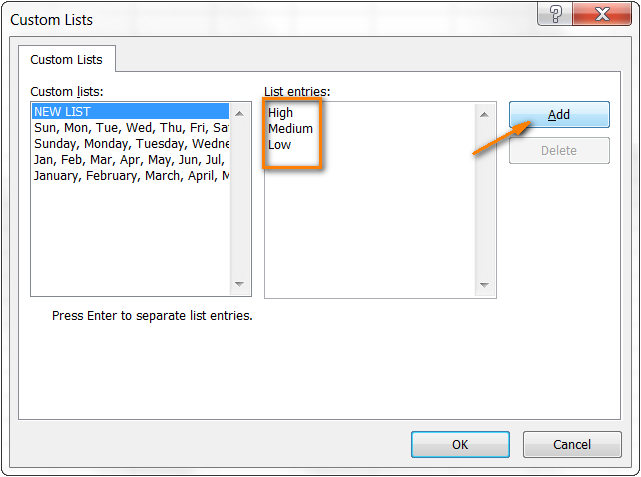
Perform steps 1 and 2 described above, and when you have the Custom Lists dialog open, select the NEW LIST in the left-hand column under Custom Lists, and type the entries directly into the List entries box on the right. Remember to type your entries exactly in the same order you want them to be sorted, from top to bottom:
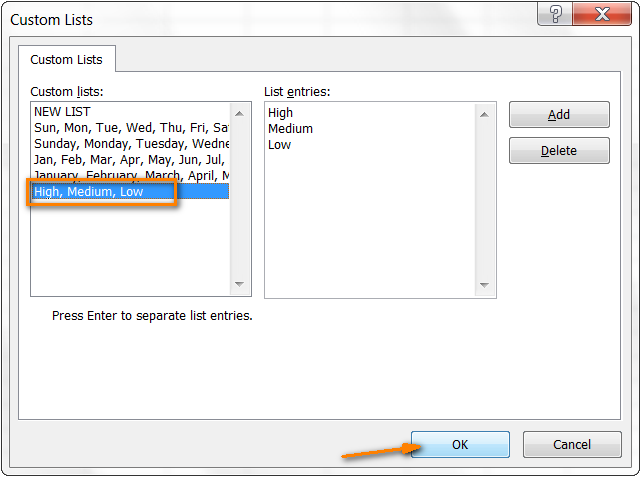
Click Add and you will see that the newly created custom list is added to the existing custom lists, then click OK:
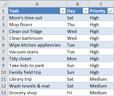
And here come our household tasks, sorted by priority:
When you use custom lists for sorting, you are free to sort by multiple columns and use a different custom list in each case. The process is exactly the same as we have already discussed when sorting by several columns.
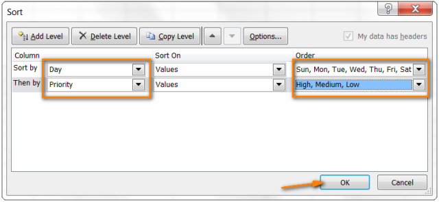
And finally, we have our weekly household chores sorted with the utmost logic, first by the day of the week, and then by priority 🙂
That’s all for today, thank you for reading!
Источник
Rows and Column in Excel (Table of Contents)
- Introduction to Rows and Column in Excel
- Rows and Column Navigation in excel
- How to Select Rows and Column in excel?
- Adjusting Column Width
Introduction to Rows and Column in Excel
In Microsoft excel, if we open a new workbook, we can see that sheet will contain tables with light grey color. Basically excel is a tabular format which contains n number of rows and columns, where rows in excel will be in a horizontal line, and column in excel will be in a vertical line.
- In excel, we can find each row by its row number, which is shown in the below screenshot, which shows vertical numbers on the left side of each sheet.
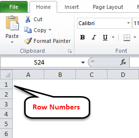
- As we can see in the above screenshot that each row can be identified by their row numbers like 1, 2, 3 etc.
- Whereas we can find the column in excel, which can be identified by the column header like A, B, C. which will be shown normally in all excel sheets, which are shown below.
- In Excel, each column is named by its header, which shows the column header horizontally at the top of the excel sheet.
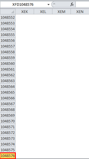
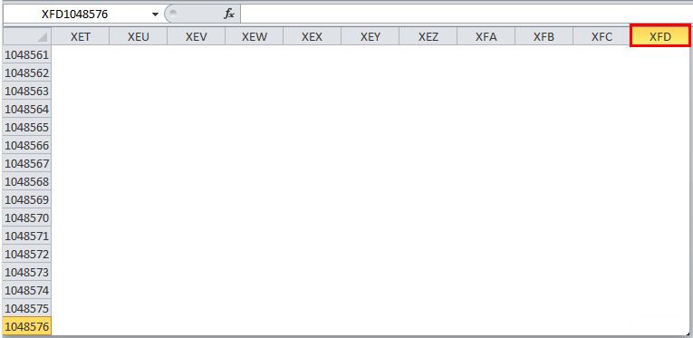
In Microsoft Excel 2010 and the latest version, we have row numbers ranging from 1 to 1048576 in 1048576, whereas the column ranges from A to XFD in a total of 16384 columns which is shown in the below screenshot.
Rows in excel range from 1 to 1048576, which is highlighted in red mark
The column in excel ranges from A to XFD, which is highlighted in red mark.
Rows and Column Navigation in excel
In this example, we will see how to navigate rows and columns with the below examples.
We can find the last row of excel by using the keyboard shortcut key CTRL+DOWN NAVIGATION ARROW KEY, or else we can use the vertical scrollbars to go to the end of the row.
We can find the last column of excel by using the CTRL+RIGHT NAVIGATION ARROW KEY, or else we can use the horizontal scrollbars to go to the end of the column.
How to Select Rows and Column in excel?
In this example, we will learn how to select the rows and columns in excel.
You can download this Rows and Column Excel Template here – Rows and Column Excel Template
Rows and Column in Excel – Example#1
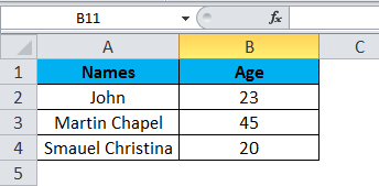
Normally, when we open a workbook, we can see that sheet contains tabular rows and columns where each row is specified by their row number and column specified by their column header.
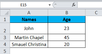
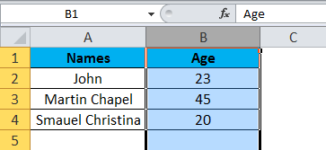
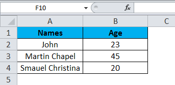
Consider the below example, which has some data in an excel sheet. Here we will see how to select the rows and columns.
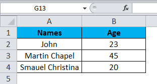
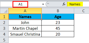
In the above screenshot, we can see that names and age column have their own header name A and B, and each row has its own row number.
In excel, each time when we select a row or column, “Name Box” will display the specific row number and column name, which is shown in the below screenshot.
In this example, we will select the Names and Age, and let’s see how the rows and column header is getting displayed.
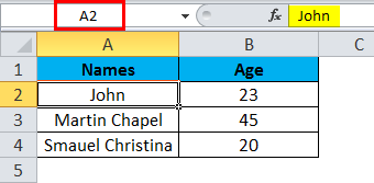
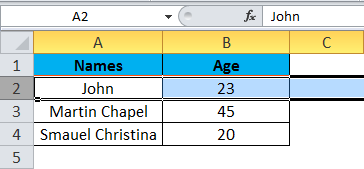
Step 1 – First, select the cell Name John.
Step 2 – Once you select the cell name, John, we will get the row number and column name as A2 in the name box, which means that we have selected A column second row as A2, shown below screenshot with yellow highlighted.
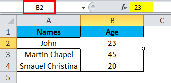
Step 3 – Now select cell 23, where it will show the selected cell is B2 which is shown in the below screenshot with yellow highlighted.
Step 4 – Now select all the names and columns to show that we have 4 rows and 2 columns shown in the below screenshot.
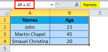
In this way, we can identify the row number and column name by selecting each cell in excel.
Example#2 – Changing Row and Column Size
This example shows how to change the row and column size by using the following examples.
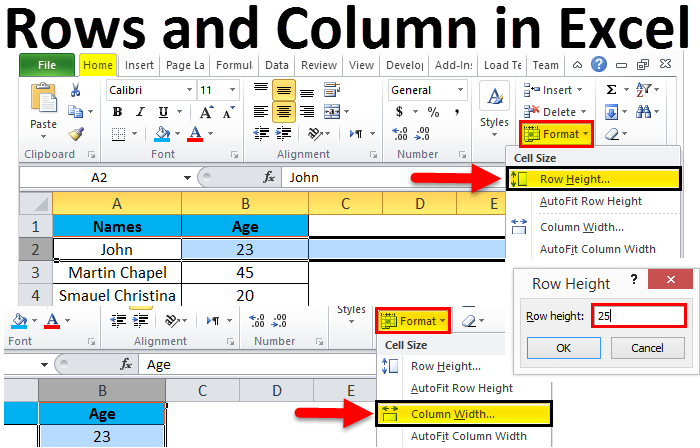
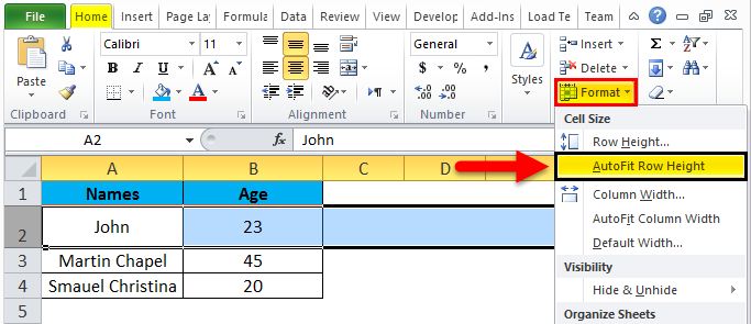
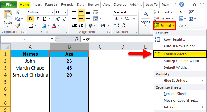
Excel row and column width size can be modified by using the format option in the HOME menu, which is shown below.
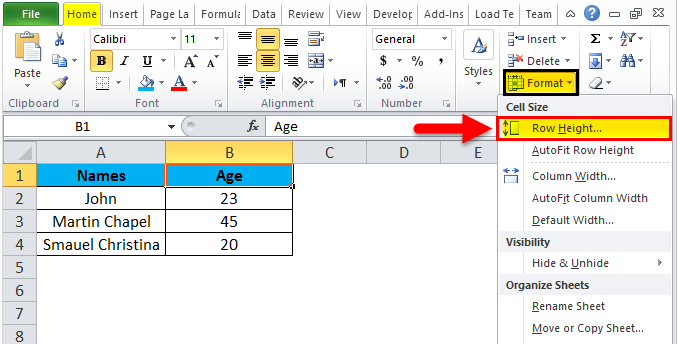
Using the format menu, we can change the row and column width where we have the list option, which are as follows:
- ROW HEIGHT– This is used to adjust the row height.
- AUTOFIT ROW HEIGHT– This will automatically adjust the row height.
- COLUMN WIDTH – This is used to adjust column width.
- AUTOFIT COLUMN WIDTH– This will automatically adjust the column width.
Let’s consider the below example to change the row and column width. Follow the below steps.
Step 1 – First, select the second row as shown in the below screenshot.
Step 2 – Go to the Format menu and click on ROW HEIGHT, as shown below.
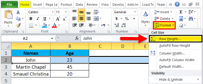
Step 3 – Once we select the ROW HEIGHT, we will get the below dialog box to change the height of the row.
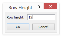
Step 4 – Now increase the row height to 25 so that the selected row height will get increased, as shown in the below screenshot.

We can see that row height has been increased when compared to the previous one; alternatively, we can change the row height by using the mouse.
Step 5 – Now go to the second option in the format list called AUTOFIT ROW HEIGHT, which will automatically reset the row to its original height.
Step 6 – Select the same row and go to the Format menu.
Step 7 – Now select the “AutoFit Row Height” as shown below.
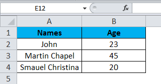
Once we click on the “AutoFit Row Height” option, the row height will reset to the original position, shown below.
Adjusting Column Width
We can adjust the column width in the same way by using the format option.
Step 1 – First, click on the cell B cell as shown below.
Step 2 – Now go to the Format menu and click on column width as shown in the below screenshot.
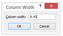
Once we click on the Column width, we will get the below dialog box to increase the column width, as shown below.
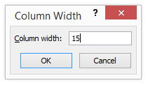
Step 3 – Now increase the column width by 15 to increase the selected column width.
In the above screenshot, we can see that column width has been increased; alternatively, we can adjust the column width by using the mouse where if we place the mouse cursor, we will get the + plus mark sign near to the column.
Step 4 – Now click on the next option called “AutoFit Column width”. So that the selected column will get reset to its original size, which is shown below.
Things to Remember
- In excel, we can delete and insert multiple rows and columns.
- We can hide the specific row and columns using the hide option.
- Row and column cells can be protected by locking the specific cells.
Recommended Articles
This has been a guide to Rows and Columns in Excel. Here we also discuss Rows and Columns in Excel along with practical examples and downloadable excel template. You can also go through our other suggested articles –
- Excel Compare Two Columns
- Unhide Columns in Excel
- Sort Columns in Excel
- Excel Columns to Rows
Updated on November 18, 2019
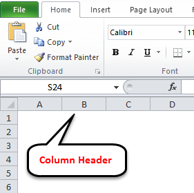
In Excel and Google Sheets, the column heading or column header is the gray-colored row containing the letters (A, B, C, etc.) used to identify each column in the worksheet. The column header is located above row 1 in the worksheet.
The row heading or row header is the gray-colored column located to the left of column 1 in the worksheet containing the numbers (1, 2, 3, etc.) used to identify each row in the worksheet.
Column and Row Headings and Cell References
Taken together, the column letters and the row numbers in the two headings create cell references which identify individual cells that are located at the intersection point between a column and row in a worksheet.
Cell references – such as A1, F56, or AC498 – are used extensively in spreadsheet operations such as formulas and when creating charts.
Printing Row and Column Headings in Excel
By default, Excel and Google Spreadsheets do not print the column or row headings seen on screen. Printing these heading rows often makes it easier to track the location of data in large, printed worksheets.
In Excel, it is a simple matter to activate the feature. Note, however, that it must be turned on for each worksheet to be printed. Activating the feature on one worksheet in a workbook will not result in the row and column headings being printed for all worksheets.
Currently, it is not possible to print column and row headings in Google Spreadsheets.
To print the column and/or row headings for the current worksheet in Excel:
- Click Page Layout tab of the ribbon.
- Click on the Print checkbox in the Sheet Options group to activate the feature.
Turning Row and Column Headings on or off in Excel
The row and column headings do not have to be displayed on a particular worksheet. Reasons for turning them off would be to improve the appearance of the worksheet or to gain extra screen space on large worksheets – possibly when taking screen captures.
As with printing, the row and column headings must be turned on or off for each individual worksheet.
To turn off the row and column headings in Excel:
- Click on the File menu to open the drop-down list.
- Click Options in the list to open the Excel Options dialog box.
- In the left-hand panel of the dialog box, click on Advanced.
- In the Display options for this worksheet section – located near the bottom of the right-hand pane of the dialog box – click on the checkbox next to the Show row and column headers option to remove the checkmark.
- To turn off the row and column headings for additional worksheets in the current workbook, select the name of another worksheet from the drop-down box located next to the Display options for this worksheet heading and clear the checkmark in the Show row and column headers checkbox.
- Click OK to close the dialog box and return to the worksheet.
Currently, it is not possible to turn column and row headings off in Google Sheets.
R1C1 References vs. A1
By default, Excel uses the A1 reference style for cell references. This results, as mentioned, in the column headings displaying letters above each column starting with the letter A and the row heading displaying numbers beginning with one.
An alternative referencing system – known as R1C1 references – is available and if it is activated, all worksheets in all workbooks will display numbers rather than letters in the column headings. The row headings continue to display numbers as with the A1 referencing system.
There are some advantages to using the R1C1 system – mostly when it comes to formulas and when writing VBA code for Excel macros.
To turn the R1C1 referencing system on or off:
- Click on the File menu to open the drop-down list.
- Click on Options in the list to open the Excel Options dialog box.
- In the left-hand panel of the dialog box, click on Formulas.
- In the Working with formulas section of the right-hand pane of the dialog box, click on the checkbox next to the R1C1 reference style option to add or remove the checkmark.
- Click OK to close the dialog box and return to the worksheet.
Changing the Default Font in Column and Row Headers in Excel
Whenever a new Excel file is opened, the row and column headings are displayed using the workbook’s default Normal style font. This Normal style font is also the default font used in all worksheet cells.
For Excel 2013, 2016, and Excel 365, the default heading font is Calibri 11 pt. but this can be changed if it is too small, too plain, or just not to your liking. Note, however, that this change affects all worksheets in a workbook.
To change the Normal style settings:
- Click on the Home tab of the Ribbon menu.
- In the Styles group, click Cell Styles to open the Cell Styles drop-down palette.
- Right-click on the box in the palette entitled Normal – this is the Normal style – to open this option’s context menu.
- Click on Modify in the menu to open the Style dialog box.
- In the dialog box, click on the Format button to open the Format Cells dialog box.
- In this second dialog box, click on the Font tab.
- In the Font: section of this tab, select the desired font from the drop-down list of choices.
- Make any other desired changes – such as Font style or size.
- Click OK twice, to close both dialog boxes and return to the worksheet.
If you do not save the workbook after making this change the font change will not be saved and the workbook will revert back to the previous font the next time it is opened.
Thanks for letting us know!
Get the Latest Tech News Delivered Every Day
Subscribe
As you begin working with data spanning over several columns and rows in Excel, you will realise that it becomes increasingly difficult to track or remember the column and row title of the cell you are reading. Sighted users can easily lookup the title visually, but a JAWS user has to move the focus to the title cell to read it. This results in some inconvenience and a reduction in productivity. Fortunately, there is a solution for this problem.
There are a couple of different ways to make JAWS read the column and/ or row titles. However, before we start discussing these ways, download the training file for this chapter: Chap 4. Cities and population.xlsx.
The training file contains 4 sheets with population statistics of several cities across India. Go ahead and open the file. The focus will be in cell A1 of worksheet named “20 most populated cities”. In this worksheet, the cities have been listed in column B from B4 to B24, and the years are listed in row 3, from C3 to M3. The state of the cities in column B is listed in column N from N4 to N24. Go ahead and move around the sheet to get a feel of the data presented.

Training file – Worksheet: 20 most populated cities
Basic method
Having spent some time in the worksheet, you would now realise why is it convenient to have the column and row titles announced to you. In order for JAWS to announce the column and row titles, you will have to first specify which column and rows contain the title.
To define which column contains titles of various rows, move to the column containing the row titles and press “INSERT+CTRL+ALT+R”. If you wish to specify which row contains the titles for various columns, move to the row containing the column titles and press “INSERT+CTRL+ALT+C”.
Let’s try this in our training file. But wait, before you go on to specify the column and/ or row containing the titles, you will have to first verify one small JAWS setting. While in the training file, press INSERT + V. This will open the JAWS Quick Setting – Excel dialog box. Type “define” in the edit box and go down to “Define Name Column and Row Title Override” and press F6. Select the option “On for the current file”, and press ESCAPE to close the dialog box.

JAWS Quick Setting – Excel dialog box
Now, we would like cities listed in column B to serve as the row titles in this worksheet. To specify this to JAWS, go anywhere in column B and press “INSERT+CTRL+ALT+R”. Similarly, to specify that row 3 contains column titles, simply go anywhere in row 3 and press “INSERT+CTRL+ALT+C”. Try moving around the worksheet. If you have done everything correctly, JAWS will announce the column and row titles to you.
Limitations of basic method
When one defines the column and row titles using the basic method, the entire column and/ or row specified by a user gets designated as the title column or row. This results in some inconvenience if a worksheet contains more than one data table. To overcome this limitation, we can use Excel’s naming function.
Specifying title regions using Excel’s naming function
Before we learn how to specify title regions using the naming function, we will have to make a few changes in JAWS settings. Press INSERT + V to open JAWS Quick Settings – Excel dialog box. Type “define” in the edit menu and move down till you reach “Define Name Column and Row Titles Override” and press F6. Verify that Define Name Column and Row Titles Override option is off. If it is not off, change it to off and press ESCAPE to close the dialog box.

JAWS Quick Setting – Excel dialog box
Note. If you are defining column and/ row title using the basic method, you will have to turn Define Name Column and Row Title Override option. Further, remember that you can’t use the basic and Excel’s naming function methods together.
To specify title regions using Excel’s naming function, follow the steps listed below:
- Move to the first cell in the column or row containing the titles. If the spreadsheet contains both row and column titles, move to the cell where these two intersect.
- Go to the FORMULAS TAB > DEFINE NAMES SUBMENU > NAME MANAGER BUTTON and press ENTER. The Name Manager dialog box opens. Now, choose NEW. The New Name dialog box opens with focus in the Name edit field.
- If the column contains row titles, type “RowTitle”. If the row contains column titles, type “ColumnTitle”. If the cell is an intersection of both row and column titles, type “Title”. Note, the words, “RowTitle”, “ColumnTitle” and “Title” are case sensitive and should be typed exactly as given here.
- Without leaving a space, type the region number, for example Region1. Don’t worry, this will be more clear when we take an example.
- Without leaving any space, type a period after the region number
- Without leaving any space, type the cell address of the top left corner cell of the region for which you are specifying the title. Hint, this will be the same cell in which you had moved to in step 1 above.
- Without leaving a space, type a period.
- Without leaving any space, type the cell address of the bottom right corner cell of the region for which you are specifying the titles.
- Without leaving a space, type a period.
- Lastly, without leaving any space, type the worksheet number in which you currently are. You can find the worksheet number by pressing INSERT + F1.
- After you press ENTER, the focus will return to the Name Manager dialog box. You will notice that the dialog box now displays the name you just defined.
- Press ESCAPE to close the dialog box
Sounds Complicated? Let’s try specifying the titles with the help of an example. First, go to the training file and move to worksheet named “Population stats-top 50 cities”. Hint, you can move between worksheets by pressing CTRL + PAGE up and CTRL + PAGE DOWN. This worksheet has 3 data regions as described below.

Training file – Worksheet: Population stats-top 50 cities
Region 1 description
The first data region presents population statistics for top 50 cities, and spans across cell B6, in top left corner, to F56, in bottom right corner. Cell B4 contains the caption for this region. Column B contains the names of various cities listed from B7 to B56. The city names serve as the row title. Row 6 contains column titles spanning across cell B6 to F6.
Region 2 description
The second region summarises the data given in first region by states/ territories. This region spans across Cell J6, in the top left corner, to O25, in bottom right corner. Cell J4 contains the caption for this region. Column J contains the names of states/ territories from J7 to J25. Row 6 contains column titles spanning across J6 to O6.
Region 3 description
The third and the last region presents the growth rate across different states based on the 50 cities listed in first region. This region spans across J32, in the top left corner, to M51, in the bottom right corner. Cell J30 contains the caption for this region. Column J contains the name of the cities from J33 to J51, and row 32 contains the column titles from J32 to M32.
Specifying row titles with Excel’s naming function
Let’s try specifying the row titles for the first region.
Step 1. Go to cell B6. Hint, you can go to cell B6 by pressing CTRL + G, typing “B6” and hitting ENTER.
Step 2. Now go to FORMULAS TAB > DEFINE NAMES SUBMENU > NAME MANAGER & press ENTER. The Name Manager dialog box will open. Now, choose New. The New Name dialog box will open with focus in the Name edit field.

Formula Manager button & Formula Manager dialog box
Step 3. Type “RowTitleRegion1.B6.F56.2” and press ENTER. Don’t worry, we will discuss this name in detail in a few minutes.

New name dialog box
Step 4. The focus is back in the Name Manager dialog box. Press ESCAPE to close the dialog box.
That’s it, you just specified the row titles for the first region. Now, let’s spend some time in understanding the name we just gave in Step 3 above.
First, we typed “RowTitle” to indicate that we wish to define, well, row titles.
Then we typed “Region1.”. This is to indicate that the titles are defined for the first region. Here the digit 1 is meant to indicate a distinct region. There is no hard and fast rule on how to name a region. However, you must use numbers and 2 different regions can’t have the same number.
We then typed “B6.F56.”. This specifies the boundaries of Region1. You would remember from our description of the first region above that, the region spans across B6, in top left corner, to F56, in bottom right corner.
Lastly, we typed “2”. This indicates the worksheet number. You can find this worksheet number by pressing INSERT + F1.
Specifying column titles with Excel’s naming function
Now let’s try specifying the column titles for the second region.
Step 1. Go to cell J6. Hint, you can go to cell J6 by pressing CTRL + G, typing “J6” and hitting ENTER.
Step 2. Now go to FORMULAS TAB > DEFINE NAMES SUBMENU > NAME MANAGER & press ENTER. The Name Manager dialog box will open. Now, choose New. The New Name dialog box will open with focus in the Name edit field.
Step 3. Type “ColumnTitleRegion2.J6.O25.2” and press ENTER. Don’t worry, we will discuss this name in detail in a few minutes.
Step 4. The focus is back in the Name Manager dialog box. Press ESCAPE to close the dialog box.
That’s it, you just specified the column titles for the second region. Now, just as we did for row titles, let’s spend some time in understanding the name we just gave in Step 3 above.
First, we typed “ColumnTitle” to indicate that we wish to define, yes you guessed it, column titles.
Then we typed “Region2.”. This is to indicate that the titles are defined for the second region. Here the digit 2 is meant to indicate a distinct region. There is no hard and fast rule on how to name a region. However, as you would remember, you must use numbers, and further, 2 different regions can’t have the same number.
We then typed “J6.O25.”. This specifies the boundaries of Region2. You would remember from our description of the second region above that, the region spans across J6, in top left corner, to O25, in bottom right corner.
Lastly, we typed “2”. This indicates the worksheet number. As you already know, you can find this worksheet number by pressing INSERT + F1.
Specifying column and row titles with Excel’s naming function
Now let’s try specifying both the column and row titles for the third region.
Step 1. Go to cell J32. Hint, you can go to cell J32 by pressing CTRL + G, typing “J32” and hitting ENTER.
Step 2. Now go to FORMULAS TAB > DEFINE NAMES SUBMENU > NAME MANAGER & press ENTER. The Name Manager dialog box will open. Now, choose New. The New Name dialog box will open with focus in the Name edit field.
Step 3. Type “TitleRegion3.J32.M51.2” and press ENTER. Don’t worry, we will discuss this name in detail in a few minutes.
Step 4. The focus is back in the Name Manager dialog box. Press ESCAPE to close the dialog box.
That’s it, you just specified both the column and row titles for the third region. Now, just as we did for row titles and column titles, let’s spend some time in understanding the name we just gave in Step 3 above.
First, we typed “Title” to indicate that we wish to define both column and row titles.
Then we typed “Region3.”. This is to indicate that the column and row titles are defined for the third region. Here the digit 3 is meant to indicate a distinct region. Remember, there is no hard and fast rule on how to name a region; except that they should be unique and should be numbers.
We then typed “J32.M51.”. This specifies the boundaries of Region3. You would remember from our description of the third region above that, the region spans across J32, in top left corner, to M51, in bottom right corner.
Lastly, we typed “2”. This indicates the worksheet number. As you already know, you can find this worksheet number by pressing INSERT + F1.
Advantages of specifying titles with Excel’s naming function
You can specify different title regions for different regions in one worksheet
Titles specified by one JAWS user are automatically available to other JAWS users making it easy to collaborate.
Titles can be specified even by a non-JAWS user thereby improving accessibility
Conclusion
There are 2 more worksheets in the training file. The third sheet, named “Population master stats” contains one data region spanning across B3, in top left corner, to N202, in bottom right corner. This region includes population statistics for 198 cities. We have already specified the column and row titles for this region using Excel’s naming functions.
The last worksheet, named “naming details”, lists down different parameters which can be used to specify column and/ or row titles for each of the regions across the 4 worksheets in this file.
To conclude, specifying column and row titles is one of the powerful features of JAWS. We strongly advise you to use this feature generously. If you have any questions, feel free to leave a comment below, and we will answer them for you.