Column and row in excel vba

“It is a capital mistake to theorize before one has data”- Sir Arthur Conan Doyle

This post covers everything you need to know about using Cells and Ranges in VBA. You can read it from start to finish as it is laid out in a logical order. If you prefer you can use the table of contents below to go to a section of your choice.

Topics covered include Offset property, reading values between cells, reading values to arrays and formatting cells.

A Quick Guide to Ranges and Cells

Function	Takes	Returns	Example	Gives
Range	cell address	multiple cells	.Range(«A1:A4»)	$A$1:$A$4
Cells	row, column	one cell	.Cells(1,5)	$E$1
Offset	row, column	multiple cells	Range(«A1:A2») .Offset(1,2)	$C$2:$C$3
Rows	row(s)	one or more rows	.Rows(4) .Rows(«2:4»)	$4:$4 $2:$4
Columns	column(s)	one or more columns	.Columns(4) .Columns(«B:D»)	$D:$D $B:$D

Download the Code

 

The Webinar

If you are a member of the VBA Vault, then click on the image below to access the webinar and the associated source code.

(Note: Website members have access to the full webinar archive.)

Introduction

This is the third post dealing with the three main elements of VBA. These three elements are the Workbooks, Worksheets and Ranges/Cells. Cells are by far the most important part of Excel. Almost everything you do in Excel starts and ends with Cells.

 
Generally speaking, you do three main things with Cells

1. Read from a cell.
2. Write to a cell.
3. Change the format of a cell.

 
Excel has a number of methods for accessing cells such as Range, Cells and Offset.These can cause confusion as they do similar things and can lead to confusion

In this post I will tackle each one, explain why you need it and when you should use it.

 
Let’s start with the simplest method of accessing cells – using the Range property of the worksheet.

Important Notes

I have recently updated this article so that is uses Value2.

You may be wondering what is the difference between Value, Value2 and the default:

' Value2
Range("A1").Value2 = 56

' Value
Range("A1").Value = 56

' Default uses value
Range("A1") = 56

 
Using Value may truncate number if the cell is formatted as currency. If you don’t use any property then the default is Value.

It is better to use Value2 as it will always return the actual cell value(see this article from Charle Williams.)

The Range Property

The worksheet has a Range property which you can use to access cells in VBA. The Range property takes the same argument that most Excel Worksheet functions take e.g. “A1”, “A3:C6” etc.

The following example shows you how to place a value in a cell using the Range property.

' https://excelmacromastery.com/
Public Sub WriteToCell()

    ' Write number to cell A1 in sheet1 of this workbook
    ThisWorkbook.Worksheets("Sheet1").Range("A1").Value2 = 67

    ' Write text to cell A2 in sheet1 of this workbook
    ThisWorkbook.Worksheets("Sheet1").Range("A2").Value2 = "John Smith"

    ' Write date to cell A3 in sheet1 of this workbook
    ThisWorkbook.Worksheets("Sheet1").Range("A3").Value2 = #11/21/2017#

End Sub

 
As you can see Range is a member of the worksheet which in turn is a member of the Workbook. This follows the same hierarchy as in Excel so should be easy to understand. To do something with Range you must first specify the workbook and worksheet it belongs to.

For the rest of this post I will use the code name to reference the worksheet.

' https://excelmacromastery.com/
Public Sub UsingCodeName()

    ' Write number to cell A1 in sheet1 of this workbook
    Sheet1.Range("A1").Value2 = 67

    ' Write text to cell A2 in sheet1 of this workbook
    Sheet1.Range("A2").Value2 = "John Smith"

    ' Write date to cell A3 in sheet1 of this workbook
    Sheet1.Range("A3").Value2 = #11/21/2017#

End Sub

You can also write to multiple cells using the Range property

' https://excelmacromastery.com/
Public Sub WriteToMulti()

    ' Write number to a range of cells
    Sheet1.Range("A1:A10").Value2 = 67

    ' Write text to multiple ranges of cells
    Sheet1.Range("B2:B5,B7:B9").Value2 = "John Smith"

End Sub

 
You can download working examples of all the code from this post from the top of this article.
 

The Cells Property of the Worksheet

The worksheet object has another property called Cells which is very similar to range. There are two differences

1. Cells returns a range of one cell only.
2. Cells takes row and column as arguments.

 
The example below shows you how to write values to cells using both the Range and Cells property

' https://excelmacromastery.com/
Public Sub UsingCells()

    ' Write to A1
    Sheet1.Range("A1").Value2 = 10
    Sheet1.Cells(1, 1).Value2  = 10

    ' Write to A10
    Sheet1.Range("A10").Value2 = 10
    Sheet1.Cells(10, 1).Value2  = 10

    ' Write to E1
    Sheet1.Range("E1").Value2 = 10
    Sheet1.Cells(1, 5).Value2  = 10

End Sub

 
You may be wondering when you should use Cells and when you should use Range. Using Range is useful for accessing the same cells each time the Macro runs.

For example, if you were using a Macro to calculate a total and write it to cell A10 every time then Range would be suitable for this task.

Using the Cells property is useful if you are accessing a cell based on a number that may vary. It is easier to explain this with an example.

 
In the following code, we ask the user to specify the column number. Using Cells gives us the flexibility to use a variable number for the column.

' https://excelmacromastery.com/
Public Sub WriteToColumn()

    Dim UserCol As Integer
    
    ' Get the column number from the user
    UserCol = Application.InputBox(" Please enter the column...", Type:=1)
    
    ' Write text to user selected column
    Sheet1.Cells(1, UserCol).Value2 = "John Smith"

End Sub

 
In the above example, we are using a number for the column rather than a letter.

To use Range here would require us to convert these values to the letter/number  cell reference e.g. “C1”. Using the Cells property allows us to provide a row and a column number to access a cell.

Sometimes you may want to return more than one cell using row and column numbers. The next section shows you how to do this.

Using Cells and Range together

As you have seen you can only access one cell using the Cells property. If you want to return a range of cells then you can use Cells with Ranges as follows

' https://excelmacromastery.com/
Public Sub UsingCellsWithRange()

    With Sheet1
        ' Write 5 to Range A1:A10 using Cells property
        .Range(.Cells(1, 1), .Cells(10, 1)).Value2 = 5

        ' Format Range B1:Z1 to be bold
        .Range(.Cells(1, 2), .Cells(1, 26)).Font.Bold = True

    End With

End Sub

 
As you can see, you provide the start and end cell of the Range. Sometimes it can be tricky to see which range you are dealing with when the value are all numbers. Range has a property called Address which displays the letter/ number cell reference of any range. This can come in very handy when you are debugging or writing code for the first time.

 
In the following example we print out the address of the ranges we are using:

' https://excelmacromastery.com/
Public Sub ShowRangeAddress()

    ' Note: Using underscore allows you to split up lines of code
    With Sheet1

        ' Write 5 to Range A1:A10 using Cells property
        .Range(.Cells(1, 1), .Cells(10, 1)).Value2 = 5
        Debug.Print "First address is : " _
            + .Range(.Cells(1, 1), .Cells(10, 1)).Address

        ' Format Range B1:Z1 to be bold
        .Range(.Cells(1, 2), .Cells(1, 26)).Font.Bold = True
        Debug.Print "Second address is : " _
            + .Range(.Cells(1, 2), .Cells(1, 26)).Address

    End With

End Sub

 
In the example I used Debug.Print to print to the Immediate Window. To view this window select View->Immediate Window(or Ctrl G)

 

 

 
You can download all the code for this post from the top of this article.
 

The Offset Property of Range

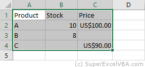
Range has a property called Offset. The term Offset refers to a count from the original position. It is used a lot in certain areas of programming. With the Offset property you can get a Range of cells the same size and a certain distance from the current range. The reason this is useful is that sometimes you may want to select a Range based on a certain condition. For example in the screenshot below there is a column for each day of the week. Given the day number(i.e. Monday=1, Tuesday=2 etc.) we need to write the value to the correct column.

 

 
We will first attempt to do this without using Offset.

' https://excelmacromastery.com/
' This sub tests with different values
Public Sub TestSelect()

    ' Monday
    SetValueSelect 1, 111.21
    ' Wednesday
    SetValueSelect 3, 456.99
    ' Friday
    SetValueSelect 5, 432.25
    ' Sunday
    SetValueSelect 7, 710.17

End Sub

' Writes the value to a column based on the day
Public Sub SetValueSelect(lDay As Long, lValue As Currency)

    Select Case lDay
        Case 1: Sheet1.Range("H3").Value2 = lValue
        Case 2: Sheet1.Range("I3").Value2 = lValue
        Case 3: Sheet1.Range("J3").Value2 = lValue
        Case 4: Sheet1.Range("K3").Value2 = lValue
        Case 5: Sheet1.Range("L3").Value2 = lValue
        Case 6: Sheet1.Range("M3").Value2 = lValue
        Case 7: Sheet1.Range("N3").Value2 = lValue
    End Select

End Sub

 
As you can see in the example, we need to add a line for each possible option. This is not an ideal situation. Using the Offset Property provides a much cleaner solution

' https://excelmacromastery.com/
' This sub tests with different values
Public Sub TestOffset()

    DayOffSet 1, 111.01
    DayOffSet 3, 456.99
    DayOffSet 5, 432.25
    DayOffSet 7, 710.17

End Sub

Public Sub DayOffSet(lDay As Long, lValue As Currency)

    ' We use the day value with offset specify the correct column
    Sheet1.Range("G3").Offset(, lDay).Value2 = lValue

End Sub

 
As you can see this solution is much better. If the number of days in increased then we do not need to add any more code. For Offset to be useful there needs to be some kind of relationship between the positions of the cells. If the Day columns in the above example were random then we could not use Offset. We would have to use the first solution.

 
One thing to keep in mind is that Offset retains the size of the range. So .Range(“A1:A3”).Offset(1,1) returns the range B2:B4. Below are some more examples of using Offset

' https://excelmacromastery.com/
Public Sub UsingOffset()

    ' Write to B2 - no offset
    Sheet1.Range("B2").Offset().Value2 = "Cell B2"

    ' Write to C2 - 1 column to the right
    Sheet1.Range("B2").Offset(, 1).Value2 = "Cell C2"

    ' Write to B3 - 1 row down
    Sheet1.Range("B2").Offset(1).Value2 = "Cell B3"

    ' Write to C3 - 1 column right and 1 row down
    Sheet1.Range("B2").Offset(1, 1).Value2 = "Cell C3"

    ' Write to A1 - 1 column left and 1 row up
    Sheet1.Range("B2").Offset(-1, -1).Value2 = "Cell A1"

    ' Write to range E3:G13 - 1 column right and 1 row down
    Sheet1.Range("D2:F12").Offset(1, 1).Value2 = "Cells E3:G13"

End Sub

Using the Range CurrentRegion

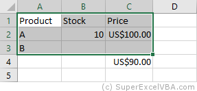
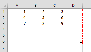
CurrentRegion returns a range of all the adjacent cells to the given range.

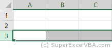
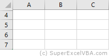
In the screenshot below you can see the two current regions. I have added borders to make the current regions clear.

A row or column of blank cells signifies the end of a current region.

You can manually check the CurrentRegion in Excel by selecting a range and pressing Ctrl + Shift + *.

If we take any range of cells within the border and apply CurrentRegion, we will get back the range of cells in the entire area.

For example
Range(“B3”).CurrentRegion will return the range B3:D14
Range(“D14”).CurrentRegion will return the range B3:D14
Range(“C8:C9”).CurrentRegion will return the range B3:D14
and so on

How to Use

We get the CurrentRegion as follows

' Current region will return B3:D14 from above example
Dim rg As Range
Set rg = Sheet1.Range("B3").CurrentRegion

Read Data Rows Only

Read through the range from the second row i.e.skipping the header row

' Current region will return B3:D14 from above example
Dim rg As Range
Set rg = Sheet1.Range("B3").CurrentRegion

' Start at row 2 - row after header
Dim i As Long
For i = 2 To rg.Rows.Count
    ' current row, column 1 of range
    Debug.Print rg.Cells(i, 1).Value2
Next i

Remove Header

Remove header row(i.e. first row) from the range. For example if range is A1:D4 this will return A2:D4

' Current region will return B3:D14 from above example
Dim rg As Range
Set rg = Sheet1.Range("B3").CurrentRegion

' Remove Header
Set rg = rg.Resize(rg.Rows.Count - 1).Offset(1)

' Start at row 1 as no header row
Dim i As Long
For i = 1 To rg.Rows.Count
    ' current row, column 1 of range
    Debug.Print rg.Cells(i, 1).Value2
Next i

 

Using Rows and Columns as Ranges

If you want to do something with an entire Row or Column you can use the Rows or Columns property of the Worksheet. They both take one parameter which is the row or column number you wish to access

' https://excelmacromastery.com/
Public Sub UseRowAndColumns()

    ' Set the font size of column B to 9
    Sheet1.Columns(2).Font.Size = 9

    ' Set the width of columns D to F
    Sheet1.Columns("D:F").ColumnWidth = 4

    ' Set the font size of row 5 to 18
    Sheet1.Rows(5).Font.Size = 18

End Sub

Using Range in place of Worksheet

You can also use Cells, Rows and Columns as part of a Range rather than part of a Worksheet. You may have a specific need to do this but otherwise I would avoid the practice. It makes the code more complex. Simple code is your friend. It reduces the possibility of errors.

 
The code below will set the second column of the range to bold. As the range has only two rows the entire column is considered B1:B2

' https://excelmacromastery.com/
Public Sub UseColumnsInRange()

    ' This will set B1 and B2 to be bold
    Sheet1.Range("A1:C2").Columns(2).Font.Bold = True

End Sub

 
You can download all the code for this post from the top of this article.
 

Reading Values from one Cell to another

In most of the examples so far we have written values to a cell. We do this by placing the range on the left of the equals sign and the value to place in the cell on the right. To write data from one cell to another we do the same. The destination range goes on the left and the source range goes on the right.

 
The following example shows you how to do this:

' https://excelmacromastery.com/
Public Sub ReadValues()

    ' Place value from B1 in A1
    Sheet1.Range("A1").Value2 = Sheet1.Range("B1").Value2

    ' Place value from B3 in sheet2 to cell A1
    Sheet1.Range("A1").Value2 = Sheet2.Range("B3").Value2

    ' Place value from B1 in cells A1 to A5
    Sheet1.Range("A1:A5").Value2 = Sheet1.Range("B1").Value2

    ' You need to use the "Value" property to read multiple cells
    Sheet1.Range("A1:A5").Value2 = Sheet1.Range("B1:B5").Value2

End Sub

 
As you can see from this example it is not possible to read from multiple cells. If you want to do this you can use the Copy function of Range with the Destination parameter

' https://excelmacromastery.com/
Public Sub CopyValues()

    ' Store the copy range in a variable
    Dim rgCopy As Range
    Set rgCopy = Sheet1.Range("B1:B5")

    ' Use this to copy from more than one cell
    rgCopy.Copy Destination:=Sheet1.Range("A1:A5")

    ' You can paste to multiple destinations
    rgCopy.Copy Destination:=Sheet1.Range("A1:A5,C2:C6")

End Sub

 
The Copy function copies everything including the format of the cells. It is the same result as manually copying and pasting a selection. You can see more about it in the Copying and Pasting Cells section.

Using the Range.Resize Method

When copying from one range to another using assignment(i.e. the equals sign), the destination range must be the same size as the source range.

Using the Resize function allows us to resize a range to a given number of rows and columns.

For example:
 

' https://excelmacromastery.com/
Sub ResizeExamples()
 
    ' Prints A1
    Debug.Print Sheet1.Range("A1").Address

    ' Prints A1:A2
    Debug.Print Sheet1.Range("A1").Resize(2, 1).Address

    ' Prints A1:A5
    Debug.Print Sheet1.Range("A1").Resize(5, 1).Address
    
    ' Prints A1:D1
    Debug.Print Sheet1.Range("A1").Resize(1, 4).Address
    
    ' Prints A1:C3
    Debug.Print Sheet1.Range("A1").Resize(3, 3).Address
    
End Sub

 
When we want to resize our destination range we can simply use the source range size.

In other words, we use the row and column count of the source range as the parameters for resizing:

' https://excelmacromastery.com/
Sub Resize()

    Dim rgSrc As Range, rgDest As Range
    
    ' Get all the data in the current region
    Set rgSrc = Sheet1.Range("A1").CurrentRegion

      ' Get the range destination
    Set rgDest = Sheet2.Range("A1")
    Set rgDest = rgDest.Resize(rgSrc.Rows.Count, rgSrc.Columns.Count)
    
    rgDest.Value2 = rgSrc.Value2

End Sub

 
We can do the resize in one line if we prefer:

' https://excelmacromastery.com/
Sub ResizeOneLine()

    Dim rgSrc As Range
    
    ' Get all the data in the current region
    Set rgSrc = Sheet1.Range("A1").CurrentRegion
    
    With rgSrc
        Sheet2.Range("A1").Resize(.Rows.Count, .Columns.Count).Value2 = .Value2
    End With
    
End Sub

Reading Values to variables

We looked at how to read from one cell to another. You can also read from a cell to a variable. A variable is used to store values while a Macro is running. You normally do this when you want to manipulate the data before writing it somewhere. The following is a simple example using a variable. As you can see the value of the item to the right of the equals is written to the item to the left of the equals.

' https://excelmacromastery.com/
Public Sub UseVariables()

    ' Create
    Dim number As Long

    ' Read number from cell
    number = Sheet1.Range("A1").Value2

    ' Add 1 to value
    number = number + 1

    ' Write new value to cell
    Sheet1.Range("A2").Value2 = number

End Sub

 
To read text to a variable you use a variable of type String:

' https://excelmacromastery.com/
Public Sub UseVariableText()

    ' Declare a variable of type string
    Dim text As String

    ' Read value from cell
    text = Sheet1.Range("A1").Value2

    ' Write value to cell
    Sheet1.Range("A2").Value2 = text

End Sub

 
You can write a variable to a range of cells. You just specify the range on the left and the value will be written to all cells in the range.

' https://excelmacromastery.com/
Public Sub VarToMulti()

    ' Read value from cell
    Sheet1.Range("A1:B10").Value2 = 66

End Sub

 
You cannot read from multiple cells to a variable. However you can read to an array which is a collection of variables. We will look at doing this in the next section.

How to Copy and Paste Cells

If you want to copy and paste a range of cells then you do not need to select them. This is a common error made by new VBA users.

Note: We normally use Range.Copy when we want to copy formats, formulas, validation. If we want to copy values it is not the most efficient method.
I have written a complete guide to copying data in Excel VBA here.

 
You can simply copy a range of cells like this:

Range("A1:B4").Copy Destination:=Range("C5")

 
Using this method copies everything – values, formats, formulas and so on. If you want to copy individual items you can use the PasteSpecial property of range.

 
It works like this

Range("A1:B4").Copy
Range("F3").PasteSpecial Paste:=xlPasteValues
Range("F3").PasteSpecial Paste:=xlPasteFormats
Range("F3").PasteSpecial Paste:=xlPasteFormulas

 
The following table shows a full list of all the paste types

Paste Type
xlPasteAll
xlPasteAllExceptBorders
xlPasteAllMergingConditionalFormats
xlPasteAllUsingSourceTheme
xlPasteColumnWidths
xlPasteComments
xlPasteFormats
xlPasteFormulas
xlPasteFormulasAndNumberFormats
xlPasteValidation
xlPasteValues
xlPasteValuesAndNumberFormats

Reading a Range of Cells to an Array

You can also copy values by assigning the value of one range to another.

Range("A3:Z3").Value2 = Range("A1:Z1").Value2

 
The value of  range in this example is considered to be a variant array. What this means is that you can easily read from a range of cells to an array. You can also write from an array to a range of cells. If you are not familiar with arrays you can check them out in this post.  

 
The following code shows an example of using an array with a range:

' https://excelmacromastery.com/
Public Sub ReadToArray()

    ' Create dynamic array
    Dim StudentMarks() As Variant

    ' Read 26 values into array from the first row
    StudentMarks = Range("A1:Z1").Value2

    ' Do something with array here

    ' Write the 26 values to the third row
    Range("A3:Z3").Value2 = StudentMarks

End Sub

 
Keep in mind that the array created by the read is a 2 dimensional array. This is because a spreadsheet stores values in two dimensions i.e. rows and columns

Going through all the cells in a Range

Sometimes you may want to go through each cell one at a time to check value.

 
You can do this using a For Each loop shown in the following code

' https://excelmacromastery.com/
Public Sub TraversingCells()

    ' Go through each cells in the range
    Dim rg As Range
    For Each rg In Sheet1.Range("A1:A10,A20")
        ' Print address of cells that are negative
        If rg.Value < 0 Then
            Debug.Print rg.Address + " is negative."
        End If
    Next

End Sub

 
You can also go through consecutive Cells using the Cells property and a standard For loop.

 
The standard loop is more flexible about the order you use but it is slower than a For Each loop.

' https://excelmacromastery.com/
Public Sub TraverseCells()
 
    ' Go through cells from A1 to A10
    Dim i As Long
    For i = 1 To 10
        ' Print address of cells that are negative
        If Range("A" & i).Value < 0 Then
            Debug.Print Range("A" & i).Address + " is negative."
        End If
    Next
 
    ' Go through cells in reverse i.e. from A10 to A1
    For i = 10 To 1 Step -1
        ' Print address of cells that are negative
        If Range("A" & i) < 0 Then
            Debug.Print Range("A" & i).Address + " is negative."
        End If
    Next
 
End Sub

Formatting Cells

Sometimes you will need to format the cells the in spreadsheet. This is actually very straightforward. The following example shows you various formatting you can add to any range of cells

' https://excelmacromastery.com/
Public Sub FormattingCells()

    With Sheet1

        ' Format the font
        .Range("A1").Font.Bold = True
        .Range("A1").Font.Underline = True
        .Range("A1").Font.Color = rgbNavy

        ' Set the number format to 2 decimal places
        .Range("B2").NumberFormat = "0.00"
        ' Set the number format to a date
        .Range("C2").NumberFormat = "dd/mm/yyyy"
        ' Set the number format to general
        .Range("C3").NumberFormat = "General"
        ' Set the number format to text
        .Range("C4").NumberFormat = "Text"

        ' Set the fill color of the cell
        .Range("B3").Interior.Color = rgbSandyBrown

        ' Format the borders
        .Range("B4").Borders.LineStyle = xlDash
        .Range("B4").Borders.Color = rgbBlueViolet

    End With

End Sub

Main Points

The following is a summary of the main points

1. Range returns a range of cells
2. Cells returns one cells only
3. You can read from one cell to another
4. You can read from a range of cells to another range of cells.
5. You can read values from cells to variables and vice versa.
6. You can read values from ranges to arrays and vice versa
7. You can use a For Each or For loop to run through every cell in a range.
8. The properties Rows and Columns allow you to access a range of cells of these types

What’s Next?

Free VBA Tutorial If you are new to VBA or you want to sharpen your existing VBA skills then why not try out the The Ultimate VBA Tutorial.

Related Training: Get full access to the Excel VBA training webinars and all the tutorials.

(NOTE: Planning to build or manage a VBA Application? Learn how to build 10 Excel VBA applications from scratch.)

---

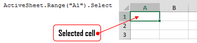
VBA Select

It is very common to find the .Select methods in saved macro recorder code, next to a Range object.

.Select is used to select one or more elements of Excel (as can be done by using the mouse) allowing further manipulation of them.

Selecting cells with the mouse:

Selecting cells with VBA:

    'Range([cell1],[cell2])
    Range(Cells(1, 1), Cells(9, 5)).Select
    Range("A1", "E9").Select
    Range("A1:E9").Select

Each of the above lines select the range from «A1» to «E9».

---

VBA Select CurrentRegion

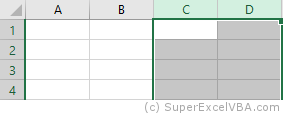
If a region is populated by data with no empty cells, an option for an automatic selection is the CurrentRegion property alongside the .Select method.

CurrentRegion.Select will select, starting from a Range, all the area populated with data.

    Range("A1").CurrentRegion.Select

Make sure there are no gaps between values, as CurrentRegion will map the region through adjoining cells (horizontal, vertical and diagonal).

  Range("A1").CurrentRegion.Select

With all the adjacent data

Not all adjacent data

«C4» is not selected because it is not immediately adjacent to any filled cells.

---

VBA ActiveCell

The ActiveCell property brings up the active cell of the worksheet.

In the case of a selection, it is the only cell that stays white.

A worksheet has only one active cell.

    Range("B2:C4").Select
    ActiveCell.Value = "Active"

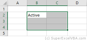
Usually the ActiveCell property is assigned to the first cell (top left) of a Range, although it can be different when the selection is made manually by the user (without macros).

The AtiveCell property can be used with other commands, such as Resize.

---

VBA Selection

After selecting the desired cells, we can use Selection to refer to it and thus make changes:

    Range("A1:D7").Select
    Selection = 7

Selection also accepts methods and properties (which vary according to what was selected).

    Selection.ClearContents 'Deletes only the contents of the selection
    Selection.Interior.Color = RGB(255, 255, 0) 'Adds background color to the selection

As in this case a cell range has been selected, the Selection will behave similarly to a Range. Therefore, Selection should also accept the .Interior.Color property.

RGB (Red Green Blue) is a color system used in a number of applications and languages. The input values for each color, in the example case, ranges from 0 to 255.

---

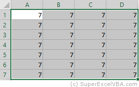
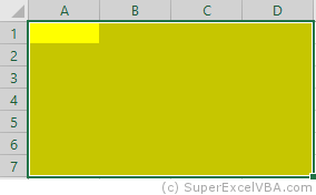
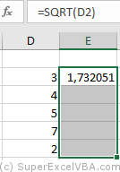
Selection FillDown

If there is a need to replicate a formula to an entire selection, you can use the .FillDown method

    Selection.FillDown

Before the FillDown

After the FillDown

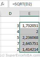
.FillDown is a method applicable to Range. Since the Selection was done in a range of cells (equivalent to a Range), the method will be accepted.

.FillDown replicates the Range/Selection formula of the first line, regardless of which ActiveCell is selected.

.FillDown can be used at intervals greater than one column (E.g. Range(«B1:C2»).FillDown will replicate the formulas of B1 and C1 to B2 and C2 respectively).

---

VBA EntireRow and EntireColumn

You can select one or multiple rows or columns with VBA.

    Range("B2").EntireRow.Select
    Range("C3:D3").EntireColumn.Select

The selection will always refer to the last command executed with Select.

To insert a row use the Insert method.

    Range("A7").EntireRow.Insert
    'In this case, the content of the seventh row will be shifted downward

To delete a row use the Delete method.

    Range("A7").EntireRow.Delete
    'In this case, the content of the eighth row will be moved to the seventh

---

VBA Rows and Columns

Just like with the EntireRow and EntireColumn property, you can use Rows and Columns to select a row or column.

    Columns(5).Select
    Rows(3).Select

To hide rows:

    Range("A1:C3").Rows.Hidden = True

In the above example, rows 1 to 3 of the worksheet were hidden.

---

VBA Row and Column

Row and Column are properties that are often used to obtain the numerical address of the first row or first column of a selection or a specific cell.

    Range("A3:H30").Row 'Referring to the row; returns 3
    Range("B3").Column  'Referring to the column; returns 2

The results of Row and Column are often used in loops or resizing.

---

---

Consolidating Your Learning

Suggested Exercise

---

---

# Ways to refer to a single cell

The simplest way to refer to a single cell on the current Excel worksheet is simply to enclose the A1 form of its reference in square brackets:

Note that square brackets are just convenient syntactic sugar (opens new window) for the Evaluate method of the Application object, so technically, this is identical to the following code:

You could also call the Cells method which takes a row and a column and returns a cell reference.

Remember that whenever you pass a row and a column to Excel from VBA, the row is always first, followed by the column, which is confusing because it is the opposite of the common A1 notation where the column appears first.

In both of these examples, we did not specify a worksheet, so Excel will use the active sheet (the sheet that is in front in the user interface). You can specify the active sheet explicitly:

Or you can provide the name of a particular sheet:

There are a wide variety of methods that can be used to get from one range to another. For example, the Rows method can be used to get to the individual rows of any range, and the Cells method can be used to get to individual cells of a row or column, so the following code refers to cell C1:

# Creating a Range

A Range (opens new window) cannot be created or populated the same way a string would:

It is considered best practice to qualify your references (opens new window), so from now on we will use the same approach here.
More about Creating Object Variables (e.g. Range) on MSDN (opens new window) . More about Set Statement on MSDN (opens new window).

There are different ways to create the same Range:

Note in the example that Cells(2, 1) is equivalent to Range(«A2»). This is because Cells returns a Range object.
Some sources: Chip Pearson-Cells Within Ranges (opens new window); MSDN-Range Object (opens new window); John Walkenback-Referring To Ranges In Your VBA Code (opens new window).

Also note that in any instance where a number is used in the declaration of the range, and the number itself is outside of quotation marks, such as Range(«A» & 2), you can swap that number for a variable that contains an integer/long. For example:

If you are using double loops, Cells is better:

# Offset Property

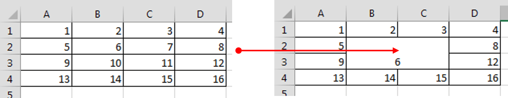
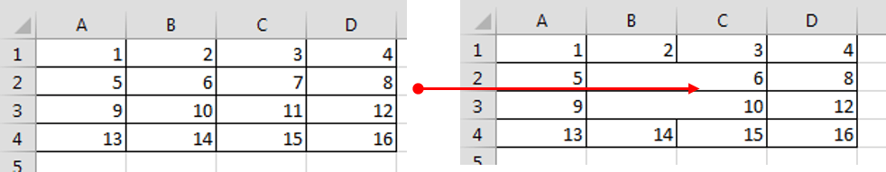
• Offset(Rows, Columns) — The operator used to statically reference another point from the current cell. Often used in loops. It should be understood that positive numbers in the rows section moves right, wheres as negatives move left. With the columns section positives move down and negatives move up.

i.e

This code selects B2, puts a new string there, then moves that string back to A1 afterwards clearing out B2.

# Saving a reference to a cell in a variable

To save a reference to a cell in a variable, you must use the Set syntax, for example:

later…

Why is the Set keyword required? Set tells Visual Basic that the value on the right hand side of the = is meant to be an object.

# How to Transpose Ranges (Horizontal to Vertical & vice versa)

Note: Copy/PasteSpecial also has a Paste Transpose option which updates the transposed cells’ formulas as well.

# Syntax

• Set — The operator used to set a reference to an object, such as a Range
• For Each — The operator used to loop through every item in a collection

Note that the variable names r, cell and others can be named however you like but should be named appropriately so the code is easier to understand for you and others.

This tutorial will demonstrate how to select and work with entire rows or columns in VBA.

First we will cover how to select entire rows and columns, then we will demonstrate how to manipulate rows and columns.

Select Entire Rows or Columns

Select Single Row

You can select an entire row with the Rows Object like this:

Rows(5).Select

Or you can use EntireRow along with the Range or Cells Objects:

Range("B5").EntireRow.Select

or

Cells(5,1).EntireRow.Select

You can also use the Range Object to refer specifically to a Row:

Range("5:5").Select

Select Single Column

Instead of the Rows Object, use the Columns Object to select columns. Here you can reference the column number 3:

Columns(3).Select

or letter “C”, surrounded by quotations:

Columns("C").Select

Instead of EntireRow, use EntireColumn along with the Range or Cells Objects to select entire columns:

Range("C5").EntireColumn.Select

or

Cells(5,3).EntireColumn.Select

You can also use the Range Object to refer specifically to a column:

Range("B:B").Select

Select Multiple Rows or Columns

Selecting multiple rows or columns works exactly the same when using EntireRow or EntireColumn:

Range("B5:D10").EntireRow.Select

or

Range("B5:B10").EntireColumn.Select

However, when you use the Rows or Columns Objects, you must enter the row numbers or column letters in quotations:

Rows("1:3").Select

or

Columns("B:C").Select

Select ActiveCell Row or Column

To select the ActiveCell Row or Column, you can use one of these lines of code:

ActiveCell.EntireRow.Select

or

ActiveCell.EntireColumn.Select

Select Rows and Columns on Other Worksheets

In order to select Rows or Columns on other worksheets, you must first select the worksheet.

Sheets("Sheet2").Select
Rows(3).Select

The same goes for when selecting rows or columns in other workbooks.

Workbooks("Book6.xlsm").Activate
Sheets("Sheet2").Select
Rows(3).Select

Note: You must Activate the desired workbook. Unlike the Sheets Object, the Workbook Object does not have a Select Method.

VBA Coding Made Easy

Stop searching for VBA code online. Learn more about AutoMacro — A VBA Code Builder that allows beginners to code procedures from scratch with minimal coding knowledge and with many time-saving features for all users!

Learn More

Is Selecting Rows and Columns Necessary?

However, it’s (almost?) never necessary to actually select Rows or Columns. You don’t need to select a Row or Column in order to interact with them. Instead, you can apply Methods or Properties directly to the Rows or Columns. The next several sections will demonstrate different Methods and Properties that can be applied.

You can use any method listed above to refer to Rows or Columns.

Methods and Properties of Rows & Columns

Delete Entire Rows or Columns

To delete rows or columns, use the Delete Method:

Rows("1:4").Delete

or:

Columns("A:D").Delete

VBA Programming | Code Generator does work for you!

Insert Rows or Columns

Use the Insert Method to insert rows or columns:

Rows("1:4").Insert

or:

Columns("A:D").Insert

Copy & Paste Entire Rows or Columns

Paste Into Existing Row or Column

When copying and pasting entire rows or columns you need to decide if you want to paste over an existing row / column or if you want to insert a new row / column to paste your data.

These first examples will copy and paste over an existing row or column:

Range("1:1").Copy Range("5:5")

or

Range("C:C").Copy Range("E:E")

Insert & Paste

These next examples will paste into a newly inserted row or column.

This will copy row 1 and insert it into row 5, shifting the existing rows down:

Range("1:1").Copy
Range("5:5").Insert

This will copy column C and insert it into column E, shifting the existing columns to the right:

Range("C:C").Copy
Range("E:E").Insert

Hide / Unhide Rows and Columns

To hide rows or columns set their Hidden Properties to True. Use False to hide the rows or columns:

'Hide Rows
Rows("2:3").EntireRow.Hidden = True

'Unhide Rows
Rows("2:3").EntireRow.Hidden = False

or

'Hide Columns
Columns("B:C").EntireColumn.Hidden = True

'Unhide Columns
Columns("B:C").EntireColumn.Hidden = False

Group / UnGroup Rows and Columns

If you want to Group rows (or columns) use code like this:

'Group Rows
Rows("3:5").Group

'Group Columns
Columns("C:D").Group

To remove the grouping use this code:

'Ungroup Rows
Rows("3:5").Ungroup

'Ungroup Columns
Columns("C:D").Ungroup

This will expand all “grouped” outline levels:

ActiveSheet.Outline.ShowLevels RowLevels:=8, ColumnLevels:=8

and this will collapse all outline levels:

ActiveSheet.Outline.ShowLevels RowLevels:=1, ColumnLevels:=1

Set Row Height or Column Width

To set the column width use this line of code:

Columns("A:E").ColumnWidth = 30

To set the row height use this line of code:

Rows("1:1").RowHeight = 30

AutoMacro | Ultimate VBA Add-in | Click for Free Trial!

Autofit Row Height / Column Width

To Autofit a column:

Columns("A:B").Autofit

To Autofit a row:

Rows("1:2").Autofit

Rows and Columns on Other Worksheets or Workbooks

To interact with rows and columns on other worksheets, you must define the Sheets Object:

Sheets("Sheet2").Rows(3).Insert

Similarly, to interact with rows and columns in other workbooks, you must also define the Workbook Object:

Workbooks("book1.xlsm").Sheets("Sheet2").Rows(3).Insert

Get Active Row or Column

To get the active row or column, you can use the Row and Column Properties of the ActiveCell Object.

MsgBox ActiveCell.Row

or

MsgBox ActiveCell.Column

This also works with the Range Object:

MsgBox Range("B3").Column

title	keywords	f1_keywords	ms.prod	api_name	ms.assetid	ms.date	ms.localizationpriority
Range object (Excel)	vbaxl10.chm143072	vbaxl10.chm143072	excel	Excel.Range	b8207778-0dcc-4570-1234-f130532cc8cd	08/14/2019	high

Range object (Excel)

Represents a cell, a row, a column, a selection of cells containing one or more contiguous blocks of cells, or a 3D range.

[!includeAdd-ins note]

Remarks

The default member of Range forwards calls without parameters to the Value property and calls with parameters to the Item member. Accordingly, someRange = someOtherRange is equivalent to someRange.Value = someOtherRange.Value, someRange(1) to someRange.Item(1) and someRange(1,1) to someRange.Item(1,1).

The following properties and methods for returning a Range object are described in the Example section:

• Range and Cells properties of the Worksheet object
• Range and Cells properties of the Range object
• Rows and Columns properties of the Worksheet object
• Rows and Columns properties of the Range object
• Offset property of the Range object
• Union method of the Application object

Example

Use Range (arg), where arg names the range, to return a Range object that represents a single cell or a range of cells. The following example places the value of cell A1 in cell A5.

Worksheets("Sheet1").Range("A5").Value = _ 
    Worksheets("Sheet1").Range("A1").Value

The following example fills the range A1:H8 with random numbers by setting the formula for each cell in the range. When it’s used without an object qualifier (an object to the left of the period), the Range property returns a range on the active sheet. If the active sheet isn’t a worksheet, the method fails.

Use the Activate method of the Worksheet object to activate a worksheet before you use the Range property without an explicit object qualifier.

Worksheets("Sheet1").Activate 
Range("A1:H8").Formula = "=Rand()"    'Range is on the active sheet

The following example clears the contents of the range named Criteria.

[!NOTE]
If you use a text argument for the range address, you must specify the address in A1-style notation (you cannot use R1C1-style notation).

Worksheets(1).Range("Criteria").ClearContents

Use Cells on a worksheet to obtain a range consisting all single cells on the worksheet. You can access single cells via Item(row, column), where row is the row index and column is the column index.
Item can be omitted since the call is forwarded to it by the default member of Range.
The following example sets the value of cell A1 to 24 and of cell B1 to 42 on the first sheet of the active workbook.

Worksheets(1).Cells(1, 1).Value = 24
Worksheets(1).Cells.Item(1, 2).Value = 42

The following example sets the formula for cell A2.

ActiveSheet.Cells(2, 1).Formula = "=Sum(B1:B5)"

Although you can also use Range("A1") to return cell A1, there may be times when the Cells property is more convenient because you can use a variable for the row or column. The following example creates column and row headings on Sheet1. Be aware that after the worksheet has been activated, the Cells property can be used without an explicit sheet declaration (it returns a cell on the active sheet).

[!NOTE]
Although you could use Visual Basic string functions to alter A1-style references, it is easier (and better programming practice) to use the Cells(1, 1) notation.

Sub SetUpTable() 
Worksheets("Sheet1").Activate 
For TheYear = 1 To 5 
    Cells(1, TheYear + 1).Value = 1990 + TheYear 
Next TheYear 
For TheQuarter = 1 To 4 
    Cells(TheQuarter + 1, 1).Value = "Q" & TheQuarter 
Next TheQuarter 
End Sub

Use_expression_.Cells, where expression is an expression that returns a Range object, to obtain a range with the same address consisting of single cells.
On such a range, you access single cells via Item(row, column), where are relative to the upper-left corner of the first area of the range.
Item can be omitted since the call is forwarded to it by the default member of Range.
The following example sets the formula for cell C5 and D5 of the first sheet of the active workbook.

Worksheets(1).Range("C5:C10").Cells(1, 1).Formula = "=Rand()"
Worksheets(1).Range("C5:C10").Cells.Item(1, 2).Formula = "=Rand()"

Use Range (cell1, cell2), where cell1 and cell2 are Range objects that specify the start and end cells, to return a Range object. The following example sets the border line style for cells A1:J10.

[!NOTE]
Be aware that the period in front of each occurrence of the Cells property is required if the result of the preceding With statement is to be applied to the Cells property. In this case, it indicates that the cells are on worksheet one (without the period, the Cells property would return cells on the active sheet).

With Worksheets(1) 
    .Range(.Cells(1, 1), _ 
        .Cells(10, 10)).Borders.LineStyle = xlThick 
End With

Use Rows on a worksheet to obtain a range consisting all rows on the worksheet. You can access single rows via Item(row), where row is the row index.
Item can be omitted since the call is forwarded to it by the default member of Range.

[!NOTE]
It’s not legal to provide the second parameter of Item for ranges consisting of rows. You first have to convert it to single cells via Cells.

The following example deletes row 5 and 10 of the first sheet of the active workbook.

Worksheets(1).Rows(10).Delete
Worksheets(1).Rows.Item(5).Delete

Use Columns on a worksheet to obtain a range consisting all columns on the worksheet. You can access single columns via Item(row) [sic], where row is the column index given as a number or as an A1-style column address.
Item can be omitted since the call is forwarded to it by the default member of Range.

[!NOTE]
It’s not legal to provide the second parameter of Item for ranges consisting of columns. You first have to convert it to single cells via Cells.

The following example deletes column «B», «C», «E», and «J» of the first sheet of the active workbook.

Worksheets(1).Columns(10).Delete
Worksheets(1).Columns.Item(5).Delete
Worksheets(1).Columns("C").Delete
Worksheets(1).Columns.Item("B").Delete

Use_expression_.Rows, where expression is an expression that returns a Range object, to obtain a range consisting of the rows in the first area of the range.
You can access single rows via Item(row), where row is the relative row index from the top of the first area of the range.
Item can be omitted since the call is forwarded to it by the default member of Range.

[!NOTE]
It’s not legal to provide the second parameter of Item for ranges consisting of rows. You first have to convert it to single cells via Cells.

The following example deletes the ranges C8:D8 and C6:D6 of the first sheet of the active workbook.

Worksheets(1).Range("C5:D10").Rows(4).Delete
Worksheets(1).Range("C5:D10").Rows.Item(2).Delete

Use_expression_.Columns, where expression is an expression that returns a Range object, to obtain a range consisting of the columns in the first area of the range.
You can access single columns via Item(row) [sic], where row is the relative column index from the left of the first area of the range given as a number or as an A1-style column address.
Item can be omitted since the call is forwarded to it by the default member of Range.

[!NOTE]
It’s not legal to provide the second parameter of Item for ranges consisting of columns. You first have to convert it to single cells via Cells.

The following example deletes the ranges L2:L10, G2:G10, F2:F10 and D2:D10 of the first sheet of the active workbook.

Worksheets(1).Range("C5:Z10").Columns(10).Delete
Worksheets(1).Range("C5:Z10").Columns.Item(5).Delete
Worksheets(1).Range("C5:Z10").Columns("D").Delete
Worksheets(1).Range("C5:Z10").Columns.Item("B").Delete

Use Offset (row, column), where row and column are the row and column offsets, to return a range at a specified offset to another range. The following example selects the cell three rows down from and one column to the right of the cell in the upper-left corner of the current selection. You cannot select a cell that is not on the active sheet, so you must first activate the worksheet.

Worksheets("Sheet1").Activate 
  'Can't select unless the sheet is active 
Selection.Offset(3, 1).Range("A1").Select

Use Union (range1, range2, …) to return multiple-area ranges—that is, ranges composed of two or more contiguous blocks of cells. The following example creates an object defined as the union of ranges A1:B2 and C3:D4, and then selects the defined range.

Dim r1 As Range, r2 As Range, myMultiAreaRange As Range 
Worksheets("sheet1").Activate 
Set r1 = Range("A1:B2") 
Set r2 = Range("C3:D4") 
Set myMultiAreaRange = Union(r1, r2) 
myMultiAreaRange.Select

If you work with selections that contain more than one area, the Areas property is useful. It divides a multiple-area selection into individual Range objects and then returns the objects as a collection. Use the Count property on the returned collection to verify a selection that contains more than one area, as shown in the following example.

Sub NoMultiAreaSelection() 
    NumberOfSelectedAreas = Selection.Areas.Count 
    If NumberOfSelectedAreas > 1 Then 
        MsgBox "You cannot carry out this command " & _ 
            "on multi-area selections" 
    End If 
End Sub

This example uses the AdvancedFilter method of the Range object to create a list of the unique values, and the number of times those unique values occur, in the range of column A.

Sub Create_Unique_List_Count()
    'Excel workbook, the source and target worksheets, and the source and target ranges.
    Dim wbBook As Workbook
    Dim wsSource As Worksheet
    Dim wsTarget As Worksheet
    Dim rnSource As Range
    Dim rnTarget As Range
    Dim rnUnique As Range
    'Variant to hold the unique data
    Dim vaUnique As Variant
    'Number of unique values in the data
    Dim lnCount As Long
    
    'Initialize the Excel objects
    Set wbBook = ThisWorkbook
    With wbBook
        Set wsSource = .Worksheets("Sheet1")
        Set wsTarget = .Worksheets("Sheet2")
    End With
    
    'On the source worksheet, set the range to the data stored in column A
    With wsSource
        Set rnSource = .Range(.Range("A1"), .Range("A100").End(xlDown))
    End With
    
    'On the target worksheet, set the range as column A.
    Set rnTarget = wsTarget.Range("A1")
    
    'Use AdvancedFilter to copy the data from the source to the target,
    'while filtering for duplicate values.
    rnSource.AdvancedFilter Action:=xlFilterCopy, _
                            CopyToRange:=rnTarget, _
                            Unique:=True
                            
    'On the target worksheet, set the unique range on Column A, excluding the first cell
    '(which will contain the "List" header for the column).
    With wsTarget
        Set rnUnique = .Range(.Range("A2"), .Range("A100").End(xlUp))
    End With
    
    'Assign all the values of the Unique range into the Unique variant.
    vaUnique = rnUnique.Value
    
    'Count the number of occurrences of every unique value in the source data,
    'and list it next to its relevant value.
    For lnCount = 1 To UBound(vaUnique)
        rnUnique(lnCount, 1).Offset(0, 1).Value = _
            Application.Evaluate("COUNTIF(" & _
            rnSource.Address(External:=True) & _
            ",""" & rnUnique(lnCount, 1).Text & """)")
    Next lnCount
    
    'Label the column of occurrences with "Occurrences"
    With rnTarget.Offset(0, 1)
        .Value = "Occurrences"
        .Font.Bold = True
    End With

End Sub

Methods

• Activate
• AddComment
• AddCommentThreaded
• AdvancedFilter
• AllocateChanges
• ApplyNames
• ApplyOutlineStyles
• AutoComplete
• AutoFill
• AutoFilter
• AutoFit
• AutoOutline
• BorderAround
• Calculate
• CalculateRowMajorOrder
• CheckSpelling
• Clear
• ClearComments
• ClearContents
• ClearFormats
• ClearHyperlinks
• ClearNotes
• ClearOutline
• ColumnDifferences
• Consolidate
• ConvertToLinkedDataType
• Copy
• CopyFromRecordset
• CopyPicture
• CreateNames
• Cut
• DataTypeToText
• DataSeries
• Delete
• DialogBox
• Dirty
• DiscardChanges
• EditionOptions
• ExportAsFixedFormat
• FillDown
• FillLeft
• FillRight
• FillUp
• Find
• FindNext
• FindPrevious
• FlashFill
• FunctionWizard
• Group
• Insert
• InsertIndent
• Justify
• ListNames
• Merge
• NavigateArrow
• NoteText
• Parse
• PasteSpecial
• PrintOut
• PrintPreview
• RemoveDuplicates
• RemoveSubtotal
• Replace
• RowDifferences
• Run
• Select
• SetCellDataTypeFromCell
• SetPhonetic
• Show
• ShowCard
• ShowDependents
• ShowErrors
• ShowPrecedents
• Sort
• SortSpecial
• Speak
• SpecialCells
• SubscribeTo
• Subtotal
• Table
• TextToColumns
• Ungroup
• UnMerge

Properties

• AddIndent
• Address
• AddressLocal
• AllowEdit
• Application
• Areas
• Borders
• Cells
• Characters
• Column
• Columns
• ColumnWidth
• Comment
• CommentThreaded
• Count
• CountLarge
• Creator
• CurrentArray
• CurrentRegion
• Dependents
• DirectDependents
• DirectPrecedents
• DisplayFormat
• End
• EntireColumn
• EntireRow
• Errors
• Font
• FormatConditions
• Formula
• FormulaArray
• FormulaHidden
• FormulaLocal
• FormulaR1C1
• FormulaR1C1Local
• HasArray
• HasFormula
• HasRichDataType
• Height
• Hidden
• HorizontalAlignment
• Hyperlinks
• ID
• IndentLevel
• Interior
• Item
• Left
• LinkedDataTypeState
• ListHeaderRows
• ListObject
• LocationInTable
• Locked
• MDX
• MergeArea
• MergeCells
• Name
• Next
• NumberFormat
• NumberFormatLocal
• Offset
• Orientation
• OutlineLevel
• PageBreak
• Parent
• Phonetic
• Phonetics
• PivotCell
• PivotField
• PivotItem
• PivotTable
• Precedents
• PrefixCharacter
• Previous
• QueryTable
• Range
• ReadingOrder
• Resize
• Row
• RowHeight
• Rows
• ServerActions
• ShowDetail
• ShrinkToFit
• SoundNote
• SparklineGroups
• Style
• Summary
• Text
• Top
• UseStandardHeight
• UseStandardWidth
• Validation
• Value
• Value2
• VerticalAlignment
• Width
• Worksheet
• WrapText
• XPath

See also

• Excel Object Model Reference

[!includeSupport and feedback]

The VBA Range Object

The Excel Range Object is an object in Excel VBA that represents a cell, row, column, a selection of cells or a 3 dimensional range. The Excel Range is also a Worksheet property that returns a subset of its cells.

Worksheet Range

The Range is a Worksheet property which allows you to select any subset of cells, rows, columns etc.

Dim r as Range 'Declared Range variable

Set r = Range("A1") 'Range of A1 cell

Set r = Range("A1:B2") 'Square Range of 4 cells - A1,A2,B1,B2

Set r= Range(Range("A1"), Range ("B1")) 'Range of 2 cells A1 and B1

Range("A1:B2").Select 'Select the Cells A1:B2 in your Excel Worksheet

Range("A1:B2").Activate 'Activate the cells and show them on your screen (will switch to Worksheet and/or scroll to this range.

Select a cell or Range of cells using the Select method. It will be visibly marked in Excel:

Working with Range variables

The Range is a separate object variable and can be declared as other variables. As the VBA Range is an object you need to use the Set statement:

Dim myRange as Range 
'...
Set myRange = Range("A1") 'Need to use Set to define myRange

The Range object defaults to your ActiveWorksheet. So beware as depending on your ActiveWorksheet the Range object will return values local to your worksheet:

Range("A1").Select
'...is the same as...
ActiveSheet.Range("A1").Select

You might want to define the Worksheet reference by Range if you want your reference values from a specifc Worksheet:

Sheets("Sheet1").Range("A1").Select 'Will always select items from Worksheet named Sheet1

The ActiveWorkbook is not same to ThisWorkbook. Same goes for the ActiveSheet. This may reference a Worksheet from within a Workbook external to the Workbook in which the macro is executed as Active references simply the currently top-most worksheet. Read more here

Range properties

The Range object contains a variety of properties with the main one being it’s Value and an the second one being its Formula.

A Range Value is the evaluated property of a cell or a range of cells. For example a cell with the formula =10+20 has an evaluated value of 20.
A Range Formula is the formula provided in the cell or range of cells. For example a cell with a formula of =10+20 will have the same Formula property.

'Let us assume A1 contains the formula "=10+20"

Debug.Print Range("A1").Value 'Returns: 30

Debug.Print Range("A1").Formula 'Returns: =10+20

Other Range properties include:
Work in progress

Worksheet Cells

A Worksheet Cells property is similar to the Range property but allows you to obtain only a SINGLE CELL, based on its row and column index. Numbering starts at 1:

The Cells property is in fact a Range object not a separate data type.
Excel facilitates a Cells function that allows you to obtain a cell from within the ActiveSheet, current top-most worksheet.

Cells(2,2).Select 'Selects B2
'...is the same as...
ActiveSheet.Cells(2,2).Select 'Select B2

Cells are Ranges which means they are not a separate data type:

Dim myRange as Range
Set myRange = Cells(1,1) 'Cell A1

Range Rows and Columns

As we all know an Excel Worksheet is divided into Rows and Columns. The Excel VBA Range object allows you to select single or multiple rows as well as single or multiple columns. There are a couple of ways to obtain Worksheet rows in VBA:

Getting an entire row or column

To get and entire row of a specified Range you need to use the EntireRow property. Although, the function’s parameters suggest taking both a RowIndex and ColumnIndex it is enough just to provide the row number. Row indexing starts at 1.
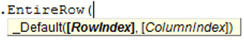To get and entire column of a specified Range you need to use the EntireColumn property. Although, the function’s parameters suggest taking both a RowIndex and ColumnIndex it is enough just to provide the column number. Column indexing starts at 1.

Range("B2").EntireRows(1).Hidden = True 'Gets and hides the entire row 2

Range("B2").EntireColumns(1).Hidden = True 'Gets and hides the entire column 2

The three properties EntireRow/EntireColumn, Rows/Columns and Row/Column are often misunderstood so read through to understand the differences.

Get a row/column of a specified range

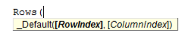If you want to get a certain row within a Range simply use the Rows property of the Worksheet. Although, the function’s parameters suggest taking both a RowIndex and ColumnIndex it is enough just to provide the row number. Row indexing starts at 1.
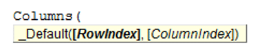Similarly you can use the Columns function to obtain any single column within a Range. Although, the function’s parameters suggest taking both a RowIndex and ColumnIndex actually the first argument you provide will be the column index. Column indexing starts at 1.

Rows(1).Hidden = True 'Hides the first row in the ActiveSheet
'same as
ActiveSheet.Rows(1).Hidden = True

Columns(1).Hidden = True 'Hides the first column in the ActiveSheet
'same as
ActiveSheet.Columns(1).Hidden = True

To get a range of rows/columns you need to use the Range function like so:

Range(Rows(1), Rows(3)).Hidden = True 'Hides rows 1:3
'same as
Range("1:3").Hidden = True
'same as 
ActiveSheet.Range("1:3").Hidden = True

Range(Columns(1), Columns(3)).Hidden = True 'Hides columns A:C
'same as
Range("A:C").Hidden = True
'same as 
ActiveSheet.Range("A:C").Hidden = True

Get row/column of specified range

The above approach assumed you want to obtain only rows/columns from the ActiveSheet – the visible and top-most Worksheet. Usually however, you will want to obtain rows or columns of an existing Range. Similarly as with the Worksheet Range property, any Range facilitates the Rows and Columns property.

Dim myRange as Range
Set myRange = Range("A1:C3")

myRange.Rows.Hidden = True 'Hides rows 1:3
myRange.Columns.Hidden = True 'Hides columns A:C

Set myRange = Range("C10:F20")
myRange.Rows(2).Hidden = True 'Hides rows 11
myRange.Columns(3).Hidden = True 'Hides columns E

Getting a Ranges first row/column number

Aside from the Rows and Columns properties Ranges also facilitate a Row and Column property which provide you with the number of the Ranges first row and column.

Set myRange = Range("C10:F20")

'Get first row number
Debug.Print myRange.Row 'Result: 10
'Get first column number
Debug.Print myRange.Column 'Result: 3

Converting Column number to Excel Column

This is an often question that turns up – how to convert a column number to a string e.g. 100 to “CV”.

Function GetExcelColumn(columnNumber As Long)
    Dim div As Long, colName As String, modulo As Long
    div = columnNumber: colName = vbNullString

    Do While div > 0
        modulo = (div - 1) Mod 26
        colName = Chr(65 + modulo) & colName
        div = ((div - modulo) / 26)
    Loop

    GetExcelColumn = colName
End Function

Range Cut/Copy/Paste

Cutting and pasting rows is generally a bad practice which I heavily discourage as this is a practice that is moments can be heavily cpu-intensive and often is unaccounted for.

Copy function

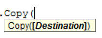The Copy function works on a single cell, subset of cell or subset of rows/columns.

'Copy values and formatting from cell A1 to cell D1
Range("A1").Copy Range("D1")

'Copy 3x3 A1:C3 matrix to D1:F3 matrix - dimension must be same
Range("A1:C3").Copy Range("D1:F3")

'Copy rows 1:3 to rows 4:6
Range("A1:A3").EntireRow.Copy Range("A4")

'Copy columns A:C to columns D:F
Range("A1:C1").EntireColumn.Copy Range("D1")

The Copy function can also be executed without an argument. It then copies the Range to the Windows Clipboard for later Pasting.

Cut function

The Cut function, similarly as the Copy function, cuts single cells, ranges of cells or rows/columns.

'Cut A1 cell and paste it to D1
Range("A1").Cut Range("D1")

'Cut 3x3 A1:C3 matrix and paste it in D1:F3 matrix - dimension must be same
Range("A1:C3").Cut Range("D1:F3")

'Cut rows 1:3 and paste to rows 4:6
Range("A1:A3").EntireRow.Cut Range("A4")

'Cut columns A:C and paste to columns D:F
Range("A1:C1").EntireColumn.Cut Range("D1")

The Cut function can be executed without arguments. It will then cut the contents of the Range and copy it to the Windows Clipboard for pasting.

Cutting cells/rows/columns does not shift any remaining cells/rows/columns but simply leaves the cut out cells empty

PasteSpecial function

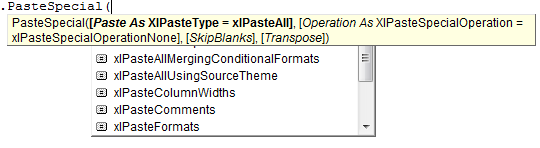The Range PasteSpecial function works only when preceded with either the Copy or Cut Range functions. It pastes the Range (or other data) within the Clipboard to the Range on which it was executed.

Syntax

The PasteSpecial function has the following syntax:

PasteSpecial( Paste, Operation, SkipBlanks, Transpose)

The PasteSpecial function can only be used in tandem with the Copy function (not Cut)

Parameters

Paste
The part of the Range which is to be pasted. This parameter can have the following values:

Parameter	Constant	Description
xlPasteSpecialOperationAdd	2	Copied data will be added with the value in the destination cell.
xlPasteSpecialOperationDivide	5	Copied data will be divided with the value in the destination cell.
xlPasteSpecialOperationMultiply	4	Copied data will be multiplied with the value in the destination cell.
xlPasteSpecialOperationNone	-4142	No calculation will be done in the paste operation.
xlPasteSpecialOperationSubtract	3	Copied data will be subtracted with the value in the destination cell.

Operation
The paste operation e.g. paste all, only formatting, only values, etc. This can have one of the following values:

Name	Constant	Description
xlPasteAll	-4104	Everything will be pasted.
xlPasteAllExceptBorders	7	Everything except borders will be pasted.
xlPasteAllMergingConditionalFormats	14	Everything will be pasted and conditional formats will be merged.
xlPasteAllUsingSourceTheme	13	Everything will be pasted using the source theme.
xlPasteColumnWidths	8	Copied column width is pasted.
xlPasteComments	-4144	Comments are pasted.
xlPasteFormats	-4122	Copied source format is pasted.
xlPasteFormulas	-4123	Formulas are pasted.
xlPasteFormulasAndNumberFormats	11	Formulas and Number formats are pasted.
xlPasteValidation	6	Validations are pasted.
xlPasteValues	-4163	Values are pasted.
xlPasteValuesAndNumberFormats	12	Values and Number formats are pasted.

SkipBlanks
If True then blanks will not be pasted.

Transpose
Transpose the Range before paste (swap rows with columns).

PasteSpecial Examples

'Cut A1 cell and paste its values to D1
Range("A1").Copy
Range("D1").PasteSpecial
 
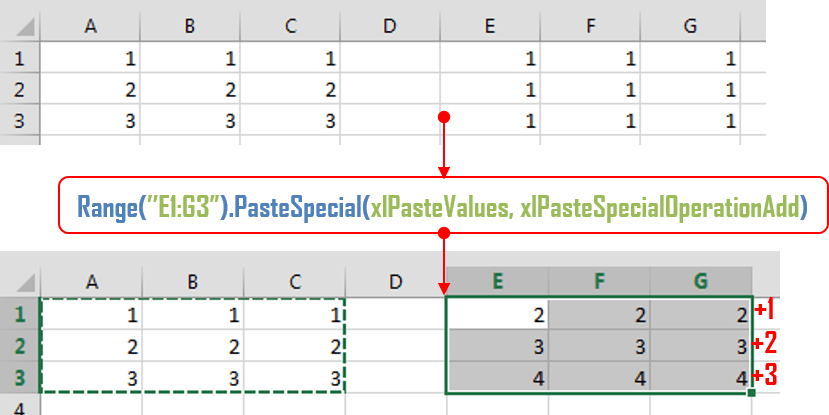
'Copy 3x3 A1:C3 matrix and add all the values to E1:G3 matrix (dimension must be same)
Range("A1:C3").Copy 
Range("E1:G3").PasteSpecial xlPasteValues, xlPasteSpecialOperationAdd

Below an example where the Excel Range A1:C3 values are copied an added to the E1:G3 Range. You can also multiply, divide and run other similar operations.

Paste

The Paste function allows you to paste data in the Clipboard to the actively selected Range. Cutting and Pasting can only be accomplished with the Paste function.

'Cut A1 cell and paste its values to D1
Range("A1").Cut
Range("D1").Select
ActiveSheet.Paste
 
'Cut 3x3 A1:C3 matrix and paste it in D1:F3 matrix - dimension must be same
Range("A1:C3").Cut 
Range("D1:F3").Select
ActiveSheet.Paste
 
'Cut rows 1:3 and paste to rows 4:6
Range("A1:A3").EntireRow.Cut 
Range("A4").Select
ActiveSheet.Paste
 
'Cut columns A:C and paste to columns D:F
Range("A1:C1").EntireColumn.Cut 
Range("D1").Select
ActiveSheet.Paste

Range Clear/Delete

The Clear function

The Clear function clears the entire content and formatting from an Excel Range. It does not, however, shift (delete) the cleared cells.

Range("A1:C3").Clear

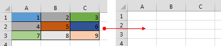
The Delete function

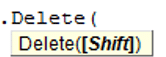The Delete function deletes a Range of cells, removing them entirely from the Worksheet, and shifts the remaining Cells in a selected shift direction.
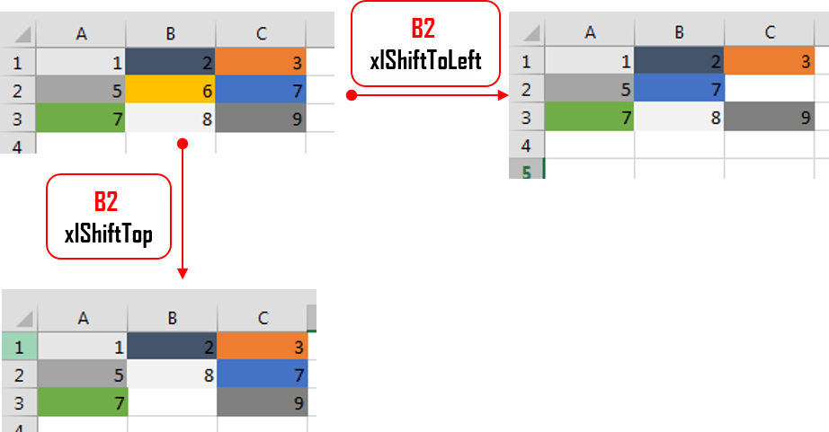
Although the manual Delete cell function provides 4 ways of shifting cells. The VBA Delete Shift values can only be either be xlShiftToLeft or xlShiftUp.

'If Shift omitted, Excel decides - shift up in this case
Range("B2").Delete 

'Delete and Shift remaining cells left
Range("B2").Delete xlShiftToLeft  

'Delete and Shift remaining cells up
Range("B2").Delete xlShiftTop

'Delete entire row 2 and shift up
Range("B2").EntireRow.Delete

'Delete entire column B and shift left
Range("B2").EntireRow.Delete

Traversing Ranges

Traversing cells is really useful when you want to run an operation on each cell within an Excel Range. Fortunately this is easily achieved in VBA using the For Each or For loops.

Dim cellRange As Range
    
For Each cellRange In Range("A1:C3")
  Debug.Print cellRange.Value
Next cellRange

Although this may not be obvious, beware of iterating/traversing the Excel Range using a simple For loop. For loops are not efficient on Ranges. Use a For Each loop as shown above. This is because Ranges resemble more Collections than Arrays. Read more on For vs For Each loops here

Traversing the UsedRange

Every Worksheet has a UsedRange. This represents that smallest rectangle Range that contains all cells that have or had at some point values. In other words if the further out in the bottom, right-corner of the Worksheet there is a certain cell (e.g. E8) then the UsedRange will be as large as to include that cell starting at cell A1 (e.g. A1:E8). In Excel you can check the current UsedRange hitting CTRL+END. In VBA you get the UsedRange like this:

ActiveSheet.UsedRange
'same as
UsedRange

You can traverse through the UsedRange like this:

Dim cellRange As Range
    
For Each cellRange In UsedRange
  Debug.Print "Row: " & cellRange.Row & ", Column: " & cellRange.Column
Next cellRange

The UsedRange is a useful construct responsible often for bloated Excel Workbooks. Often delete unused Rows and Columns that are considered to be within the UsedRange can result in significantly reducing your file size. Read also more on the XSLB file format here

Range Addresses

The Excel Range Address property provides a string value representing the Address of the Range.

Syntax

Below the syntax of the Excel Range Address property:

Address( [RowAbsolute], [ColumnAbsolute], [ReferenceStyle], [External], [RelativeTo] )

Parameters

RowAbsolute
Optional. If True returns the row part of the reference address as an absolute reference. By default this is True.

$D$10:$G$100 'RowAbsolute is set to True
$D10:$G100 'RowAbsolute is set to False

ColumnAbsolute
Optional. If True returns the column part of the reference as an absolute reference. By default this is True.

$D$10:$G$100 'ColumnAbsolute is set to True
D$10:G$100 'ColumnAbsolute is set to False

ReferenceStyle
Optional. The reference style. The default value is xlA1. Possible values:

Constant	Value	Description
xlA1	1	Default. Use xlA1 to return an A1-style reference
xlR1C1	-4150	Use xlR1C1 to return an R1C1-style reference

External
Optional. If True then property will return an external reference address, otherwise a local reference address will be returned. By default this is False.

$A$1 'Local
[Book1.xlsb]Sheet1!$A$1 'External

RelativeTo
Provided RowAbsolute and ColumnAbsolute are set to False, and the ReferenceStyle is set to xlR1C1, then you must include a starting point for the relative reference. This must be a Range variable to be set as the reference point.

Merged Ranges

Merged cells are Ranges that consist of 2 or more adjacent cells. To Merge a collection of adjacent cells run Merge function on that Range.

The Merge has only a single parameter – Across, a boolean which if True will merge cells in each row of the specified range as separate merged cells. Otherwise the whole Range will be merged. The default value is False.

Merge examples

To merge the entire Range:

'This will turn of any alerts warning that values may be lost
Application.DisplayAlerts = False

Range("B2:C3").Merge

This will result in the following:

To merge just the rows set Across to True.

'This will turn of any alerts warning that values may be lost
Application.DisplayAlerts = False

Range("B2:C3").Merge True

This will result in the following:

Remember that merged Ranges can only have a single value and formula. Hence, if you merge a group of cells with more than a single value/formula only the first value/formula will be set as the value/formula for your new merged Range

Checking if Range is merged

To check if a certain Range is merged simply use the Excel Range MergeCells property:

Range("B2:C3").Merge

Debug.Print Range("B2").MergeCells 'Result: True

The MergeArea

The MergeArea is a property of an Excel Range that represent the whole merge Range associated with the current Range. Say that $B$2:$C$3 is a merged Range – each cell within that Range (e.g. B2, C3..) will have the exact same MergedArea. See example below:

Range("B2:C3").Merge
Debug.Print Range("B2").MergeArea.Address 'Result: $B$2:$C$3

Named Ranges

Named Ranges are Ranges associated with a certain Name (string). In Excel you can find all your Named Ranges by going to Formulas->Name Manager. They are very useful when working on certain values that are used frequently through out your Workbook. Imagine that you are writing a Financial Analysis and want to use a common Discount Rate across all formulas. Just the address of the cell e.g. “A2”, won’t be self-explanatory. Why not use e.g. “DiscountRate” instead? Well you can do just that.

Creating a Named Range

Named Ranges can be created either within the scope of a Workbook or Worksheet:

Dim r as Range
'Within Workbook
Set r = ActiveWorkbook.Names.Add("NewName", Range("A1"))
'Within Worksheet
Set r = ActiveSheet.Names.Add("NewName", Range("A1"))

This gives you flexibility to use similar names across multiple Worksheets or use a single global name across the entire Workbook.

Listing all Named Ranges

You can list all Named Ranges using the Name Excel data type. Names are objects that represent a single NamedRange. See an example below of listing our two newly created NamedRanges:

Call ActiveWorkbook.Names.Add("NewName", Range("A1"))
Call ActiveSheet.Names.Add("NewName", Range("A1"))

Dim n As Name
For Each n In ActiveWorkbook.Names
  Debug.Print "Name: " & n.Name & ", Address: " & _
       n.RefersToRange.Address & ", Value: "; n.RefersToRange.Value
Next n

'Result:
'Name: Sheet1!NewName, Address: $A$1, Value:  1 
'Name: NewName, Address: $A$1, Value:  1 

SpecialCells

SpecialCells are a very useful Excel Range property, that allows you to select a subset of cells/Ranges within a certain Range.

Syntax

The SpecialCells property has the following syntax:

SpecialCells( Type, [Value] )

Parameters

Type
The type of cells to be returned. Possible values:

Constant	Value	Description
xlCellTypeAllFormatConditions	-4172	Cells of any format
xlCellTypeAllValidation	-4174	Cells having validation criteria
xlCellTypeBlanks	4	Empty cells
xlCellTypeComments	-4144	Cells containing notes
xlCellTypeConstants	2	Cells containing constants
xlCellTypeFormulas	-4123	Cells containing formulas
xlCellTypeLastCell	11	The last cell in the used range
xlCellTypeSameFormatConditions	-4173	Cells having the same format
xlCellTypeSameValidation	-4175	Cells having the same validation criteria
xlCellTypeVisible	12	All visible cells

Value
If Type is equal to xlCellTypeConstants or xlCellTypeFormulas this determines the types of cells to return e.g. with errors.

Constant	Value
xlErrors	16
xlLogical	4
xlNumbers	1
xlTextValues	2

SpecialCells examples

Get Excel Range with Constants

This will return only cells with constant cells within the Range C1:C3:

For Each r In Range("A1:C3").SpecialCells(xlCellTypeConstants)
  Debug.Print r.Value
Next r

Search for Excel Range with Errors

For Each r In ActiveSheet.UsedRange.SpecialCells(xlCellTypeFormulas, xlErrors)
  Debug.Print r.Address
Next r

Introduction to Range and Cells in VBA

When you look around in an Excel workbook, you will find that everything works around cells. A cell and a range of cells are where you store your data, and then everything starts.

To make the best of VBA, you need to learn how to use cells and ranges in your codes. For this, you need to have a solid understanding of Range objects. By using it, you can refer to cells in your codes in the following ways:

• A single cell.
• A range of cells
• A row or a column
• A three-dimensional range

The RANGE OBJECT is a part of Excel’s Object Hierarchy: Application ➜ Workbooks ➜ Worksheets ➜ Range and besides inside the worksheet. So if you are writing code to refer to the RANGE object it would be like this:

Application.Workbook(“Workbook-Name”).Worksheets(“Sheet-Name”).Range

By referring to a cell or range of cells, you can do the following things:

• You can read the value from it.
• You can enter a value in it.
• And, you can make changes to the format.

To do all these things, you need to learn to refer to a cell or a range of cells, and in the next section of this tutorial, you will learn to refer to a cell using different ways.

To refer to a cell or a range of cells, you can use three different ways.

• Range Property
• Cells Property
• Offset Property

Well, which one is best out of these depends on your requirement, but it is worth learning all three so that you can choose which one is perfect for you.

So let’s get started.

Range Property

Range property is the most common and popular way to refer to a range in your VBA codes. With Range property, you simply need to refer to the cell address. Let me tell you the syntax.

expression.range(address)

Here the expression is a variable representing a VBA object. So if you need to refer to the cell A1, the line of code you need to write would be:

Application.Workbook(“Book1”).Worksheets(“Sheet1”).Range(“A1”)

The above code tells VBA that you are referring to cell A1 which is in the worksheet “Sheet1” and workbook ”Book1”.

Note: Whenever you type a cell address in the range object, make sure to wrap it in double quotation marks. But here’s one thing to understand. As you are using VBA in Excel there’s no need to use the word “Application”. So the code would be:

Workbook(“Book1”).Worksheets(“Sheet1”).Range(“A1”)

And if you are in the Book1 there you can further trim down your code:

Worksheets(“Sheet1”).Range(“A1”)

But, if you are already in the worksheet “Sheet1” then you can further trim down your code and can only use:

Range(“A1”)

Now, let’s say if you want to refer to a full range of cells (i.e., multiple cells) you need to write the code in the following way:

Range("A1:A5")

In the above code, you have referred to the range A1 to A5 which consists of the five cells. You can also refer to a named range using the range object. Let’s say you have named range with the name of “Sales Discount” to refer to this you can write a code like this:

Range("Sales Discount")

If you want to refer to a non-continues range then you need to do something like this:

Range("A1:B5,D5:G10")

And if you want to refer to an entire row or a column then you need to enter code like the below:

Range("1:1")
Range("A:A")

At this point, you have a clear understanding of how to refer to a cell and the range of cells. But to make it best with this you need to learn how to use this to do other things.

1. Select and Activate a Cell

If you want to select a cell then you can use the Range. Select method. Let’s say if you want to select cell A5 then all you need to do is specify the range and then add “.Select” after that.

Range(“A1”).Select

This code tells VBA to select cell A5 and if you want to select a range of cells then you just need to refer to that range and simply add “.Select” after that.

Range(“A1:A5”).Select

There’s also another method that you can use to activate a cell.

Range(“A1”).Activate

Here you need to remember that you can activate only one cell at a time. Even if you specify a range with the “.Activate” method, it will select that range but the active cell will be the first cell of the range.

2. Enter a Value in a Cell

By using the range property you can enter a value in a cell or a range of cells. Let’s understand how it works using a simple example:

Range("A1").Value = "ExcelChamps"

In the above example, you have specified the A1 as a range and after that, you have added “.Value” which tells VBA to access the value property of the cell.

The next thing you have is the equals sign and then the value which you want to enter (you need to use double quotation marks if you are entering a text value). For a number, the code would like this:

Range("A1").Value = 9988

And if you want to enter a value into a range of cells, I mean multiple cells, then all you need to do is specify that range. 

Range("A1:A5").Value = "ExcelChamps"

And, here’s the code if you are referring to the non-continues range.

Range("A1:A5 , E2:E3").Value = "ExcelChamps"

3. Copy and Paste a Cell/Range

With Range property, you can use the “.Copy” method to copy and cell and then paste it into a destination cell. Let’s say if you need to copy the cell A5 the code for this would be:

Range("A5").Copy 

When you run this code it will simply copy cell A5 but the next thing is to paste this copied cell to a destination cell. For this, you need to add the keyword destination after it and followed by the cell where you want to paste it. So if you want to copy cell A1 and then want to paste it to the cell E5, the code would be:

Range("A1").Copy Destination:=Range("E5")

In the same way, if you are dealing with a range of multiple cells then the code would be like:

Range("A1:A5").Copy Destination:=Range("E5:E9")

If you have copied a range of cells and then if you have mentioned one cell as the destination range, VBA will copy the entire copied range the starting from the cell you have specified as a destination.

Range("A1:A5").Copy Destination:=Range("B1")

When you run the above code, VBA will copy range A1:A5 and will paste it to the B1:B5 even though you have mentioned only B1 as the destination range.

Tip: Just like the “.Copy” method you can use the “.Cut” method to cut a cell and then simply use a destination to paste it.

4. Use Font Property with Range Property

With the range property, you can access the font property of a cell which helps you to change all the font settings. There are a total of 18 different properties for the font which you can access. Let’s say if you want to make the text BOLD in cell A1, the code would be:

Range("A1").Font.Bold = True

This code tells VBA to access the BOLD property of the font which is inside the range A1 and you have set this property to TRUE. Now, let’s say you want to apply strikethrough to cell A1, this time the code would be:

As I said there are a total of 18 different properties you can use, so make sure to check out all of these to see which one is useful for you.

5. Clear Formatting from a Cell

By using the “.ClearFormats” method you can remove only the format from a cell or a range of cells. All you need to do is add “.ClearFormat” after specifying the range, like below:

Range("A1").ClearFormats

When you run the code above it clears all the formatting from cell A1 and if you want to do it for an entire range, you know what to do, Right?

Range("A1:A5").ClearFormats

Now the above code will simply remove the formatting from the range A1 to A5.

Cells Property

Apart from the RANGE property, you can use the “Cells” property to refer to a cell or a range of cells in your worksheet. In cell property, instead of using the cell reference, you need to enter the column number and row number of the cell.

expression.Cells(Row_Number, Column_Number)

Here the expression is a VBA object and Row_Number is the row number of the cell and Column_Number is the column of the cell. So if you want to refer to the cell A5 you can use the code below code:

Cells(5,1)

Now, this code tells VBA to refer to the cell which is at row number five and at column number one. As its syntax says you need to enter column number as address but the reality is you can also use the column alphabet if you want just by wrapping it in double quotation marks.

The below code will also refer to the cell A5:

Cells(5,"A")

And to VBA to select it simply add “.Select” at the end.

Cells(5,1).Select

The above code will select cell A5 which is in the 5th row and in the first column of the worksheet.

OFFSET Property

If you want to play well with ranges in VBA you need to know how to use the OFFSET property. It helps to refer to a cell that is a particular number of rows and columns away from another cell.

Let’s say your active cell is B5 right now and you want to navigate to the cell which is 3 columns right and 1 row down from B5, you can do this OFFSET. Below is the syntax which you need to use for the OFFSET:

expression.Offset (RowOffset, ColumnOffset)

• RowOffset: In this argument, you need to specify a number that will tell VBA how many rows you want to navigate. A positive number defines a row downward and a negative number defines a row upward.
• ColumnOffset: In this argument, you need to specify a number that will tell VBA how many columns you want to navigate. A positive number defines a column to the right and a negative number defines a left. 

Let’s write a simple code for example which we have discussed above.

1. First, you need to define the range from where you want to navigate and so type the below code:
   
2. After that, type “.Offset” and enter opening parentheses, just like below:
   
3. Next, you need to enter the row number and then the column number where you want to navigate.
   
4. In the end, you need to add “.Select” to tell VBA to select the cell where you want to navigate.
   

So when you run this code it will select the cell which is one row down and 3 columns right from cell B5.

Resize a Range using OFFSET

OFFSET not only allows you to navigate to a cell, but you can also resize the range further. Let’s continue the above example.

Range("B5").Offset(1, 3).Select

The above code navigates you to cell E6, and now let’s say you need to select the range of cells that consists of the five columns and three rows from the E6. So what you need to do is after using OFFSET, use the resize property by adding “.Resize”.

Range("B5").Offset(1, 3).Resize

Now you need to enter the row size and column size. Type a starting parenthesis and enter the number to define the row size and then a number to define the column size.

Range("B5").Offset(1, 3).Resize(3,5)

In the end, add “.Select” to tell VBA to select the range, and when you run this code, it will select the range.

Range("B5").Offset(1, 3).Resize(3, 5).Select

So, when you run this code, it will select the range E6 to I8.

Range("A1").Font.Strikethrough = True