You’ll typically find the ROW(S) or COLUMN(S) functions nested inside other functions because they make formulas more efficient to write. However, many users get caught out by these functions because you don’t edit the cell references in the same way you might with other formulas.
Watch the Video

Download Workbook
Enter your email address below to download the sample workbook.
By submitting your email address you agree that we can email you our Excel newsletter.
You’ve probably seen a formula like this before:
=VLOOKUP($B16,$B$4:$D$13,COLUMNS($B4:C4),0)
Or this:
=INDEX($C$3:$H$8,ROWS($A$3:A4),COLUMNS($A$1:B1))
And you may have even emailed me to ask “what is the ROWS/COLUMNS function doing in this formula”. The short answer is it’s returning a number, or in multi-cell array formulas, a series of consecutive numbers.
Why do you use them? Because it’s an efficient way to write formulas that require copying down columns, across rows, or both.
Just take the VLOOKUP formula above; the COLUMNS function is returning the col_index_num argument. Remember the syntax for VLOOKUP is:
=VLOOKUP(lookup_value, table_array, col_index_num, [range_lookup])
Here’s the formula again:
=VLOOKUP($B16,$B$4:$D$13,COLUMNS($B4:C4),0)
COLUMNS evaluates to 2 because it returns the number of columns in a range:
=VLOOKUP($B16,$B$4:$D$13,2,0)
And when you copy that formula across to the next column it becomes:
=VLOOKUP($B16,$B$4:$D$13,COLUMNS($B4:D4),0)
Which evaluates to:
=VLOOKUP($B16,$B$4:$D$13,3,0)
So, you can see that using COLUMNS in the col_index_num argument of your VLOOKUP formula enables you to copy and paste it across the row and it will automatically increase the next col_index_num by 1, without so much as an F2 to edit the formula.
Now we have a rough idea of how these functions work and why you’d use them, let’s understand the four functions you can use.
ROW, ROWS, COLUMN and COLUMNS
ROWS Function
The ROWS function returns the number of rows in a range:
=ROWS(A3:A6) returns 4 because there are 4 rows in the range A3:A6.
Note; the column reference is actually irrelevant, which means you could also write this formula as ROWS(3:6) or more likely, ROWS($3:6). That way row 3 is absolute (anchored), and when you copy the formula to consecutive rows the formula will become ROWS($3:7) and so on.
ROW Function
The ROW function returns the row number of a reference:
=ROW(A3) returns 3 i.e. A3 is on row 3.
Note: you can’t write this as ROW(3) but you can write ROW(3:3). And ROW() will return the number of its own row.
COLUMNS Function
The COLUMNS function returns the number of columns in a range:
=COLUMNS(B2:D2) returns 3 because there are 3 columns in the range B2:D2.
Similar to ROWS the row number for the COLUMNS function is irrelevant, which means you could also write this formula as COLUMNS(B:D) or COLUMNS($B:D).
COLUMN Function
The COLUMN function returns the column number of a reference:
=COLUMN(C2) returns 3 because column C is the third column.
Note: you can’t write COLUMN(C) but you can write COLUMN(C:C). And COLUMN() will return the number of its own column.
The key with getting the desired results from these functions is the correct use of Absolute Cell Referencing.
Use Excel ROWS and COLUMNS Functions in Array Formulas
Typically people get caught out when editing array formulas which contain one of these functions.
Let’s take this example below where the formula in column C is a multi-cell array formula that is returning the 3 smallest values from cells A1:A6:
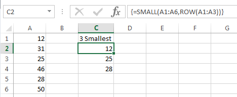
The SMALL formula evaluates like so:
=SMALL(A1:A6,ROW(A1:A3))
=SMALL({12;31;25;46;28;50},{1;2;3})
In this case ROW is returning a series of sequential numbers from 1 to 3 and as a result cell C2 returns the smallest value, cell C3 returns the second smallest and cell C4 returns the third smallest.
Problems arise when people try to edit formulas like this that they’ve copied them from somewhere, maybe another workbook, or somewhere they’ve found in a Google search.
Excel experience tells us to adjust range references to suit our data, so let’s say your data is in cells B2:B7 like so:
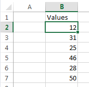
You might be tempted to copy the formula above and edit it to suit your data like this:
=SMALL(B2:B7,ROW(B2:B4))
After all, if you’re changing A1:A6 to B2:B7 for SMALL shouldn’t you also change A1:A3 to B2:B4 for ROW? NO. If you do you’ll end up with this:
=SMALL({12;31;25;46;28;50},{2;3;4})
Which would be correct for the values in cells B2:B7 but not for the ROW function reference, which as you can see above now incorrectly returns 2, 3, 4.
The correct formula is:
=SMALL(B2:B7,ROW(B1:B3))
=SMALL({12;31;25;46;28;50},{1;2;3})
Because we want the 3 smallest values, not the 2nd, 3rd and 4th smallest.
So, now you know why ROW, ROWS, COLUMN and COLUMN are typically used you’ll be able to use them in your own formulas and not get caught out editing formulas that already use these clever functions.
Caution
Pay particular attention to how these functions adjust when rows or columns are inserted above (or to the left for COLUMN/COLUMNS), or in between cells containing these formulas as it can yield unexpected results (read; formula errors).
Absolute referencing is your ally but the approach differs depending on whether you’re using these functions in an array formula or a regular formula.
Here are some tips; the formulas below will adjust as a result of rows/columns being inserted above/to the left but they will still return the same results:
Regular Formulas
=ROWS($A$1:A1) or =ROWS($1:1)
=COLUMNS($A$1:A1) or =COLUMNS($A:A)
Copy and paste (or fill) the above formulas to extend the range.
Array Formulas
=ROW(A1:A10)-ROW(A1)+1
=COLUMN(A1:J1)-COLUMN(A1)+1
The above formulas will return the numbers 1 to 10. Adjust the range referenced to suit your needs.
Examples of Formulas that use ROW(S) or COLUMN(S) Functions
VLOOKUP with dynamic column index
Summarise monthly data into quarters
Lookup and return multiple matches
List missing numbers in a sequence
Find a column containing a specific value
Remove blank cells from a range
In this article, we are going to see the details about Excel ROW, ROWS, COLUMN, COLUMNS functions, and their usages.
ROW Function
The ROW( ) function basically returns the row number for a reference.
Syntax:
=ROW([reference])
Example :
=ROW(G100); Returns 100 as output
as G100 is in the 100th row in the Excel sheet
If we write no argument inside the ROW( ) it will return the row number of the cell in which we have written the formula.
Here the following returns are achieved:
=ROW(A67) // Returns 67
=ROW(B4:H7) // Returns 4
ROWS Function
It is the extended version of the ROW function. ROWS function is used to return the number of rows in a cell range.
Syntax:
=ROWS([array])
Example :
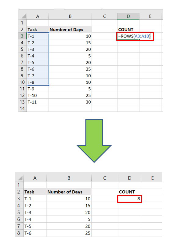
=ROWS(A2:A11) // Returns 10 as there are ten rows
It is important to note that writing the column name is trivial here. We can also write :
=ROWS(2:13) // Returns 12
COLUMN Function
The column function usually returns the column number of a reference. There are 16,384 columns in Excel from the 2007 version. It returns the value 1 to 16,384.
Syntax:
=COLUMN([reference])
Example :
=COLUMN(E20) // Returns 5 as output
as E is the fifth column in the Excel sheet
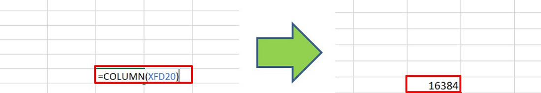
Last Column of Excel
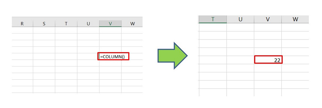
Similar to the ROW function, the argument is not mandatory. If we don’t write any argument, it will return the index of the column in which the formula is written.
COLUMNS Function
It is the extended version of the COLUMN( ). It returns the number of columns for a given cell range.
Syntax:
=COLUMNS([array])
Example :
=COLUMNS(B12:E12) // Returns 4 as output as
there are 4 columns in the given range
It is important to note that writing the row number is trivial here. We can also write :
=COLUMNS(B:E) // Returns 4
ROWS And COLUMNS Functions in Array Formulas
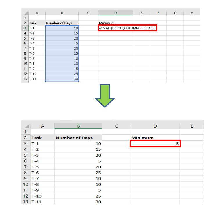
We can use the ROWS( ) and COLUMNS( ) in array formulas using SMALL( ), LARGE( ), VLOOKUP( ) functions in Excel.
Example :
The smallest value is returned to the provided cell range.
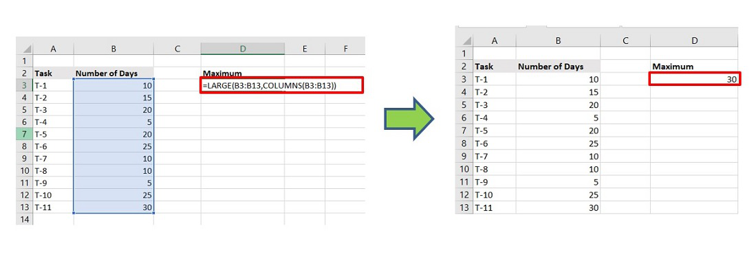
The largest value is returned to the provided cell range.
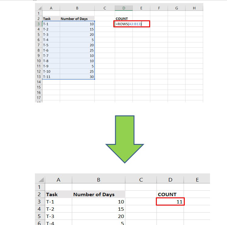
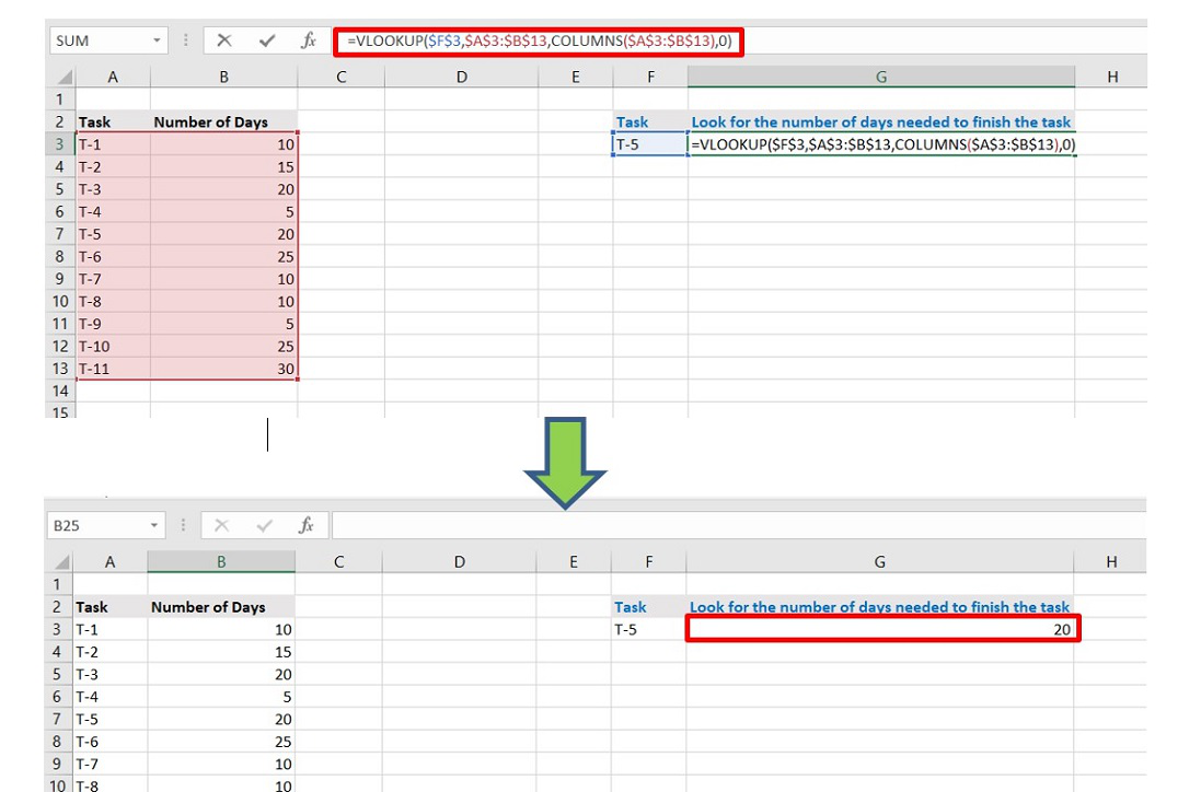
Say, we need to find the number of days needed to complete Task number 5.
The steps are :
Step 1: Choose any cell and write the name of the Task.
Step 2: Beside that cell write the “Formula” as shown below to get the “Number of Days” need :
=VLOOKUP($F$3,$A$3:$B$13,COLUMNS($A$3:$B$13),0)
F3 : Reference of the Task T-5
A3:B13 : Cell range of the entire table for VLOOKUP to search
Step 3: Click Enter.
Now, it can be observed it returns 20 as output which is perfect as per the data set.
-
Learn Excel
Use ROWS() and COLUMNS() formulas to generate numbers in a sequence [quick tip]
-
Last updated on August 17, 2009

Chandoo
Here is a quick excel formula tip to start your week.
Use ROWS() and COLUMNS() formulas next time you need sequential numbers.
What does ROWS() excel formula do?
ROWS excel formula takes a range as an argument and tells you how many rows are there in that range. For. eg. ROWS(A1:A10) gives 10.
How can you use ROWS() formula to generate sequential numbers?
Simple. Assuming you want to have the sequential numbers in range B1:B10, in B1 write =ROWS($B$1:B1) and copy down the formula in the range in B1:B10. You will now have sequential numbers in that range.
But this is lame. I could just enter the numbers myself.
You are right. Using the ROWS () to just generate sequential numbers is lame.
But in most scenarios, we need sequential numbers to do something else (like passing them to an INDEX or OFFSET formula). Often we use helper column with the sequential numbers to do this. But by using ROWS() formula, you can remove the need for helper column and easily scale your formulas.
See this example:
Actual question on PHD forums: Fill down a formula with increment
Hi, I need help on filling a formula down with a constant increment. I would like the first cell to be ‘=+B1’ the next to be ‘=+B4’ the next to be ‘=+B7’ etc… so that the increment is 3. How can this be accomplished?
Actual answer using ROWS()
in Column C, write: =+offset($b$1,rows($C$1:C1)*3,0)) and copy down
There are lots of interesting uses for ROWS() formula.
Similarly, you can use COLUMNS() formula when your data is across columns.
PS: I just crossed my personal record for hard disk crashes in a week. Now my work laptop is on the bed too.
PPS: There are more than 100 posts on the PHD Forums already. Lots of interesting questions and answers to day to day excel problems.
PPPS: Posting will be thin this week. I have composed the next installment of project management and spreadcheats series during the weekend. But the posts are in the work laptop. So wait (and pray)
PPPPS: Have a fun week ahead. 🙂
Share this tip with your colleagues

Get FREE Excel + Power BI Tips
Simple, fun and useful emails, once per week.
Learn & be awesome.
-
26 Comments -
Ask a question or say something… -
Tagged under
columns(), increment, Learn Excel, Microsoft Excel Formulas, numbers, OFFSET(), quick tip, rows(), spreadcheats, tricks
-
Category:
Learn Excel

Welcome to Chandoo.org
Thank you so much for visiting. My aim is to make you awesome in Excel & Power BI. I do this by sharing videos, tips, examples and downloads on this website. There are more than 1,000 pages with all things Excel, Power BI, Dashboards & VBA here. Go ahead and spend few minutes to be AWESOME.
Read my story • FREE Excel tips book


Excel School made me great at work.
5/5

From simple to complex, there is a formula for every occasion. Check out the list now.

Calendars, invoices, trackers and much more. All free, fun and fantastic.

Power Query, Data model, DAX, Filters, Slicers, Conditional formats and beautiful charts. It’s all here.

Still on fence about Power BI? In this getting started guide, learn what is Power BI, how to get it and how to create your first report from scratch.

- Excel for beginners
- Advanced Excel Skills
- Excel Dashboards
- Complete guide to Pivot Tables
- Top 10 Excel Formulas
- Excel Shortcuts
- #Awesome Budget vs. Actual Chart
- 40+ VBA Examples
Related Tips
26 Responses to “Use ROWS() and COLUMNS() formulas to generate numbers in a sequence [quick tip]”
-
 Jon says:
 COLUMNS() can also be helpful within a VLOOKUP to dynamically define what you call the «return_what» term in your «plain english» explanation: =VLOOKUP(what, where, return_what, [my_list_is_sorted])
Simply replace the hard-coded «return_what» number with COLUMN($C1:$F1), where $C1 is in the «what» column and «$F1» is in the «return_what» column. That way, you can add and delete columns on your table without breaking the VLOOKUP formula!
-
jeff weir says:
Good thing about the ROWS arguement is that it’s a good substitute for just the simple ROW arguement, because as you’ve structured it above with absolute_reference:relative_reference format i.e. =ROWS($B$1:B1) then it isnt going to be stuffed up if you insert another row higher up in the spreadsheet.
-
[…] can simplify the +1, +2..+11 part by using COLUMNS formula to generate the sequential numbers for […]
-
Paul Grenier says:
Chandoo,
Happy New Year to you and your beautiful family.
It was only a few months ago I needed to use VLOOKUP in an amortization schedule. With the help from one of your emails on VLOOKUP I was able to get through it.
I can’t find the lesson that was specific on understanding and using VLOOKUP.
Is there something you could email me on VLOOKUP. I think your email on this subject was around March or 2010.
Continued success in 2011.
Paul -
J MACKEY III says:
=(ROW(C4)*3)-2
Does not require a helper column. The equation can be improved by adding a cell reference.
=(ROW(C4)*$A$1)-($A$1-1)
-
[…] The ROWS($A$1:A1) portion generates continuous numbers from 1 thru 100 and thus we get next 100 13ths. For more on this technique, read – Using ROWS() to generate a series of numbers […]
-
KAUSHAL says:
Data validation in cell
i have entry 5digit Alpha,then4 digit number, then1 digit Alpha
-
Vijay Kumar Bhardwaj says:
=IF(LEN(B6)=10,IF(AND(SUMPRODUCT(—(CODE(MID(B6,{1,2,3,4,5,10},1))>=65),—(CODE(MID(B6,{1,2,3,4,5,10},1))=48),—(CODE(MID(B6,{6,7,8,9},1))<=57))=4),»OK»,»NOT OK»),»NOT OK»)
Use this formula to validate the authentication
Vijay Kumar Bhardwaj
Whatsapp :- +919463006767 -
Vijay Kumar Bhardwaj says:
=AND(LEN(SUBSTITUTE(A1,» «,»»))=10,ISTEXT(LEFT(SUBSTITUTE(A1,» «,»»),5)),ISNUMBER(N(MID(SUBSTITUTE(A1,» «,»»),6,4))),ISTEXT(RIGHT(SUBSTITUTE(A1,» «,»»),1)))
There is another Formula to validate
Whatsapp : +919463006767
-
-
[…] of typing all the 28/29 numbers, we can use ROW formula to generate these, […]
-
[…] Learn more about: using ROWS / COLUMNS formula to generate running numbers. […]
-
Keith Jones says:
I am trying to add a column of number sequentially in excel 2010, my problem is that the rows are filtered, so instead of the serial number on the extreme left running numerically it will jump numbers.
See below 383,384,406,426 if I now try to add a sequential number and drag it down by using the right handle bar the first number is just repeated and doesn’t increase.How do I get around this issue?
Thanks
-
@Keith
In the column you want to have a running 1, 2, 3…
I’ll assume Column C
In C2: add a Function =SUBTOTAL(103,$B$2:B2)
Copy down to the end of your data-
Keith Jones says:
Hi Thanks, I still cant get the function to work
column is G
and the row starts at 66,67,69,then jumps to 324 jumps again to 328 etc.
I entered the formula in to G66 and it only shows the formula in the cell and in the cells I drag it into.
Thanks
-
-
-
Eileen Cook says:
Hello. I have a database with company names in one field but the client would like each company to have the same sequence number.
For example, if we have 10 rows with the same company name, they would like all those to have the same sequence number of 1, and so on.
Need a formula so i’m not having to go through 50,000 records and group manually.-
@Eileen Cook
Sort your data by the Company Name (Column A)
Then add a new Column Sequence Number (Column B)
I’ll assume the first company is in Row 2
In B2 put 1
In B3 =IF(A3A2,B2+1,B2)
Copy down-
Eileen Cook says:
you rock!! I was missing the darn number ONE in B3 lol
Thank YOU so much.
xoxoox
-
-
-
john carr says:
I’ve updated to Excel 2013. it automatically adds a row of «column #» after the column label and before the first case. I cannot delete this row. How can I remove it?
Then I copied just cases data to a new sheet and dang Excel again added a row with cell formulas yielding an error since it refers to sheet 1 dang row of «column#». I can’t delete those cell values permanently nor delete the row. -
Elijah says:
I have an excel 2013 spreadsheet 1st row has 2 last names and first names, 2nd row has email. I want to split that information to have the first names in the first row and the last names in the second row. Please help.
-
ron says:
Hello, I just want to drag a formula down that will pull the values from a row. I’ve got the month/year in one row on a second sheet (column a, b ,c d, etc.), and on the first sheet I want to enter a formula that will pull each value to the cells in a row (a1, a2, a3, a4, ect.) any thoughts?
-
@Ron
On sheet1 in A1: =Offset(Sheet1!$A$1,,Columns($A$1:A1))
Drag down
-
-
Jim says:
SUM(R[-7]C[-2]*R[-7]C)+SUM(R[-6]C[-2]*R[-6]C)+SUM(R[-4]C[-2]*R[-4]C)
Please explain this formula to me.
Thanks
-
Craig says:
hi pretty simple query here I am thinking ?
If I have two columns the left one an increasing number of the rows containing data to the right of it and the right column some data entered.
How do I get the numbered column to automatically increase its value when data is entered into the right column next to it when it was blank?
Thanks for your time and any suggestions or tips would be most welcome.
regards Craig
-
Rich says:
Hi All,
I’m trying to figure out how to reference the second row of data in a table rather than the first, but it’s also in a different row. We recently switched to clocking out for lunch and it’s throwing off my reports which previously just had 1 clock in and 1 clock out time for each employee.
I need to reference the first clock in, and second clock out. How can I do so?
-
Abdullahi says:
Using ms excel for seating timetable in an examination where you have five different courses in a session
Leave a Reply
На чтение 4 мин. Просмотров 478 Опубликовано 18.09.2019
Функция ROW в Excel возвращает номер строки ссылки. Функция COLUMN возвращает номер столбца. Примеры в этом уроке показывают, как использовать эти функции ROW и COLUMN.
Примечание . Инструкции в этой статье относятся к Excel 2019, Excel 2016, Excel 2013, Excel 2010, Excel 2019 для Mac, Excel 2016 для Mac, Excel для Mac 2011 и Excel Online.
Содержание
- Использование функции ROW и COLUMN
- Синтаксис и аргументы функций ROW и COLUMN
- Пример 1 – опустить ссылочный аргумент с помощью функции ROW
- Пример 2 – Использование ссылочного аргумента с функцией COLUMN
Использование функции ROW и COLUMN
Функция ROW используется для:
- Вернуть номер для строки данной ссылки на ячейку.
- Вернуть номер строки для ячейки, в которой находится функция на листе.
- Возвращает ряд чисел, идентифицирующих номера всех строк, где находится функция, при использовании в формуле массива.
Функция COLUMN используется для:
- Вернуть номер столбца для ячейки, в которой находится функция на листе.
- Вернуть номер для столбца данной ссылки на ячейку.
На листе Excel строки пронумерованы сверху вниз, причем строка 1 является первой строкой. Столбцы нумеруются слева направо, причем столбец A является первым столбцом.
Следовательно, функция ROW возвращает номер 1 для первой строки и 1 048 576 для последней строки листа.
Синтаксис и аргументы функций ROW и COLUMN

Синтаксис функции относится к макету функции и включает в себя имя функции, скобки и аргументы.
Синтаксис для функции ROW:
= СТРОКА (ссылка)
Синтаксис для функции COLUMN:
= COLUMN (ссылка)
Ссылка (необязательно). Ячейка или диапазон ячеек, для которых требуется вернуть номер строки или букву столбца.
Если ссылочный аргумент опущен, происходит следующее:
- Функция ROW возвращает номер строки ссылки на ячейку, в которой находится функция (см. Строку 2 в приведенных выше примерах).
- Функция COLUMN возвращает номер столбца ссылки на ячейку, в которой находится функция (см. Строку 3 в приведенных выше примерах).
Если для аргумента Reference введен диапазон ссылок на ячейки, функция возвращает номер строки или столбца первой ячейки в предоставленном диапазоне (см. Строки 6 и 7 в приведенных выше примерах).
Пример 1 – опустить ссылочный аргумент с помощью функции ROW

В первом примере (см. Строку 2 в приведенных выше примерах) пропускается аргумент Reference и возвращается номер строки в зависимости от расположения функции на листе.
Как и в большинстве функций Excel, функция может быть введена непосредственно в активную ячейку или введена с помощью диалогового окна функции.
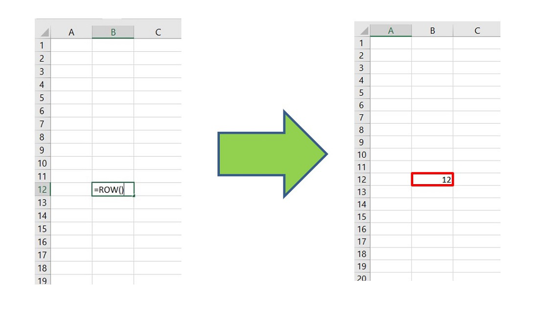
Выполните следующие шаги, чтобы ввести функцию в активную ячейку:
- Выберите ячейку B2 , чтобы сделать ее активной.
- Введите формулу = ROW () в ячейку.
- Нажмите клавишу Enter на клавиатуре, чтобы завершить функцию.
Число 2 появляется в ячейке B2, так как функция находится во втором ряду рабочего листа.
Когда вы выбираете ячейку B2, полная функция = ROW () появляется на панели формул над рабочим листом.
Пример 2 – Использование ссылочного аргумента с функцией COLUMN

Во втором примере (см. Строку 3 в приведенных выше примерах) возвращается буква столбца ссылки на ячейку (F4), введенной в качестве аргумента ссылки для функции.
- Выберите ячейку B5 , чтобы сделать ее активной.
- Выберите вкладку Формулы .
- Выберите Поиск и справка , чтобы открыть раскрывающийся список функций.
- Выберите СТОЛБЦ в списке, чтобы открыть диалоговое окно «Аргументы функций».
- В диалоговом окне поместите курсор в строку Ссылка .
- Выберите ячейку F4 на листе, чтобы ввести ссылку на ячейку в диалоговом окне.
- Выберите ОК , чтобы завершить функцию и вернуться к рабочему листу.
Число 6 появляется в ячейке B5, поскольку ячейка F4 расположена в шестом столбце (столбец F) рабочего листа.
При выборе ячейки B5 полная функция = COLUMN (F4) появляется на панели формул над рабочим листом.
Поскольку в Excel Online нет вкладки «Формулы» на ленте, вы можете использовать следующий метод, который работает во всех версиях Excel.

- Выберите ячейку B5 , чтобы сделать ее активной.
- Нажмите кнопку Вставить функцию рядом с панелью формул.
- Выберите Поиск и справка в списке категорий.
- Выберите Столбец в списке и выберите ОК .
- Выберите ячейку F4 на листе, чтобы ввести ссылку на ячейку.
- Нажмите клавишу Ввод .
Число 6 появляется в ячейке B5, поскольку ячейка F4 расположена в шестом столбце (столбец F) рабочего листа.
При выборе ячейки B5 полная функция = COLUMN (F4) появляется на панели формул над рабочим листом.
Excel 2021 Excel 2019 Excel 2016 Excel 2013 Office for business Excel 2010 More…Less
Summary
When you use the Microsoft Excel products listed at the bottom of this article, you can use a worksheet formula to covert data that spans multiple rows and columns to a database format (columnar).
More Information
The following example converts every four rows of data in a column to four columns of data in a single row (similar to a database field and record layout). This is a similar scenario as that which you experience when you open a worksheet or text file that contains data in a mailing label format.
Example
-
In a new worksheet, type the following data:
A1: Smith, John
A2: 111 Pine St.
A3: San Diego, CA
A4: (555) 128-549
A5: Jones, Sue
A6: 222 Oak Ln.
A7: New York, NY
A8: (555) 238-1845
A9: Anderson, Tom
A10: 333 Cherry Ave.
A11: Chicago, IL
A12: (555) 581-4914 -
Type the following formula in cell C1:
=OFFSET($A$1,(ROW()-1)*4+INT((COLUMN()-3)),MOD(COLUMN()-3,1))
-
Fill this formula across to column F, and then down to row 3.
-
Adjust the column sizes as necessary. Note that the data is now displayed in cells C1 through F3 as follows:
Smith, John
111 Pine St.
San Diego, CA
(555) 128-549
Jones, Sue
222 Oak Ln.
New York, NY
(555) 238-1845
Anderson, Tom
333 Cherry Ave.
Chicago, IL
(555) 581-4914
The formula can be interpreted as
OFFSET($A$1,(ROW()-f_row)*rows_in_set+INT((COLUMN()-f_col)/col_in_set), MOD(COLUMN()-f_col,col_in_set))
where:
-
f_row = row number of this offset formula
-
f_col = column number of this offset formula
-
rows_in_set = number of rows that make one record of data
-
col_in_set = number of columns of data
Need more help?
Want more options?
Explore subscription benefits, browse training courses, learn how to secure your device, and more.
Communities help you ask and answer questions, give feedback, and hear from experts with rich knowledge.
How to Convert Rows to Columns in Excel?
There are two different methods for converting rows to columns in Excel, which are as follows:
- Method #1 – Transposing Rows to Columns Using Paste Special.
- Method #2 – Transposing Rows to Columns Using TRANSPOSE Formula.
Table of contents
- How to Convert Rows to Columns in Excel?
- #1 Using Paste Special
- Example
- #2 Using TRANSPOSE Formula
- Example
- Advantages
- Disadvantages
- Things to Remember
- Recommended Articles
- #1 Using Paste Special
#1 Using Paste Special
It is an efficient method; it is easy to implement and saves time. Also, this method would be ideal if you want your original formatting to be copied.
You can download this Convert Rows to Columns Excel Template here – Convert Rows to Columns Excel Template
Example
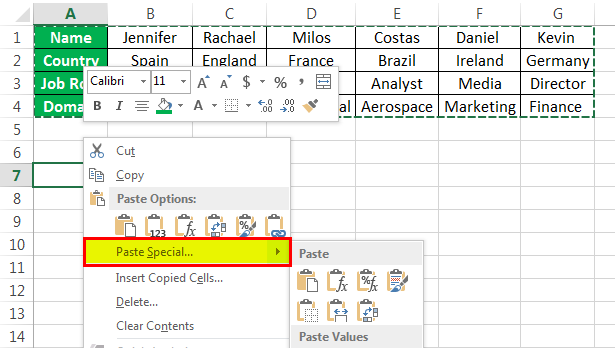
For example, if you have below data of key industry players from various regions, it also shows their job roles as shown in figure1.
| Name | Jennifer | Racheal | Milos | Costas | Daniel | Kevin |
| Country | Spain | England | France | Brazil | Ireland | Germany |
| Job Role | CTO | CEO | Analyst | Analyst | Media | Director |
| Domain | Electronics | Chemical | Mechanical | Aerospace | Marketing | Finance |
In example 1, the players’ names are written in column form. Still, the list becomes too long, and the data entered also seems unorganized. Hence, we would change the rows to columns using paste special methodsPaste special in Excel allows you to paste partial aspects of the data copied. There are several ways to paste special in Excel, including right-clicking on the target cell and selecting paste special, or using a shortcut such as CTRL+ALT+V or ALT+E+S.read more.
The steps to convert rows to columns in Excel using the Paste Special method are as follows:
- Select the whole data which needs to be transformed or transposed. Then, Copy the selected data by simply pressing Ctrl + C keys.

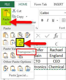
- Select a blank cell and ensure it is outside the original data range. Paste the data by pressing the “Ctrl +V” keys starting at the first blank space or cell. Then, select the down arrow from the toolbar under the “Paste” option and select “Paste Transpose.” But the easy way is to right-click the blank you chose first to paste the data. Then, select “Paste Special” from it.

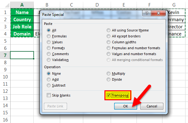
- Then, a “Paste Special” dialog box will appear from which select the “Transpose” option. And click “OK.”

- In the above figure, copy the data which needs to be transposed and then click on the down arrow of the Paste option and form the options select Transpose. (Paste-Transpose)

It shows how the transpose function is performed to convert rows to columns.


#2 Using TRANSPOSE Formula
When a user wants to keep the same connections of the rotating table with the original table, it can use a transposing method using a formula. This method is also quicker in converting rows to columns in Excel. But, it does not keep the source formatting and links it to a transposed table.
Example
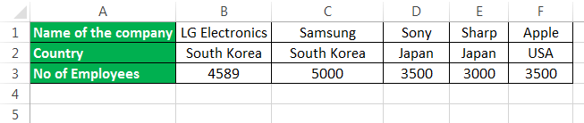
Consider the example below, as shown in figure 6, where it shows the company’s names, location, and the number of employees.
The steps to transpose rows to columns in excel using formula are as follows:
- First, count the number of rows and columns in your original excel table. And then, select the same number of blank cells but ensure you have to transpose the rows to columns to choose the blank cells in the opposite direction. Like in example 2, the number of rows is 3, and the number of columns is 6. So, you will select 6 blank rows and 3 blank columns.
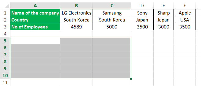
- In the first empty cell, enter the TRANSPOSE formula in excelThe TRANSPOSE function in excel helps rotate (switch) the values from rows to columns and vice versa. Being a part of the Excel lookup and reference functions, its purpose is to organize the data in the desired format. To execute the formula, the exact size of the range to be transposed is selected and the CSE key (“Control+Shift+Enter”) is pressed.
read more ‘=TRANSPOSE($A$1:$F$3)’.
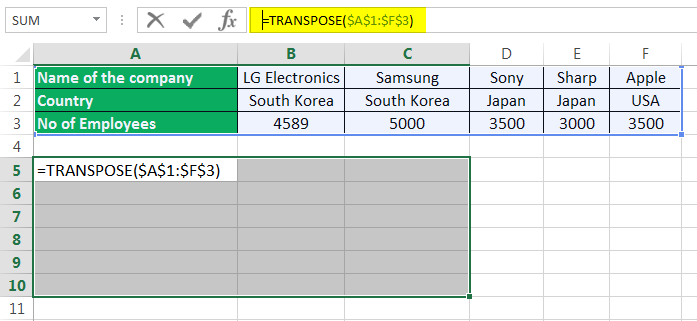
- Since this formula needs to be applied for other blank cells so press ‘Ctrl+Shift+Enter.’
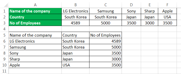
The rows are converted to columns.
Advantages
- The Paste Special method is useful when the user needs the original formatting to be continued.
- In the transpose method, by using the TRANSPOSE function, the converted table will change its data automatically, which means that whenever the user changes the data in the original table, it will automatically change the data in the transposed table, as it is linked to it.
- Converting the rows to columns in Excel sometimes helps the user to make the audience understand their data easily and so that the audience interprets it without much effort.
Disadvantages
- If the number of rows and columns increases, then the transpose method using the Paste Special options cannot perform efficiently. In this case, the “TRANSPOSE” function will be disabled when there are many rows to be converted to columns.
- The “Transpose Paste Special” option does not link the original data to the transposed data. Therefore, if you need to change the data, you must repeat all the steps.
- In the transpose method, the source formatting is not kept the same for the transposed data by using the formula.
- After converting the rows to columns in Excel using a formula, the user cannot edit the data in the transposed table as it is linked to the source data.
Things to Remember
- We can transpose rows to columns using Paste Special methods. We can link the data to the original data by selecting “Paste Link” from the “Paste Special” dialog box.
- We can also use Excel’s INDIRECT formula and ADDRESS functions in ExcelThe address function finds the cell’s address and returns an absolute value. It requires two mandatory arguments: the row number and the column number. For example, if we use =Address(1,2), the result will be $B$1.read more to convert rows to columns and vice-versa.
Recommended Articles
This article is a guide to Convert Rows to Columns in Excel. Here, we discuss switching rows to columns in Excel using the Paste Special and TRANSPOSE formula, practical examples, and a downloadable Excel template. You may learn more about Excel from the following articles: –
- Group Columns in ExcelIn Excel, grouping one or more columns together in a worksheet is referred to as group column and I t allows you to contract or expand the column.read more
- Compare Two Columns in ExcelTwo columns in excel are compared when their entries are studied for similarities and differences.read more
- Use Columns Formula in Excel
- Column Sort in Excel
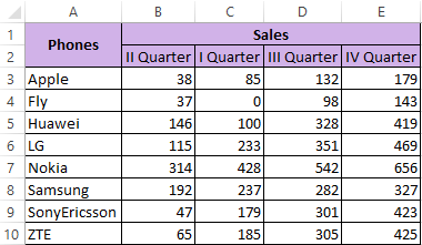
Sorting the data in Excel is a tool for presenting information in a user-friendly form. Numerical values can be sorted in ascending and descending order, text values can be sorted alphabetically and in reverse order. Available options are the sorting by color and font, in random order, according to several conditions. Columns and rows are sorted.
Sorting order in Excel
There are two ways to open the sort menu:
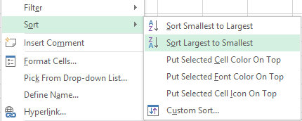
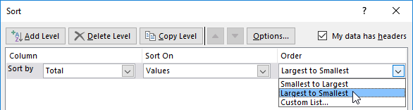
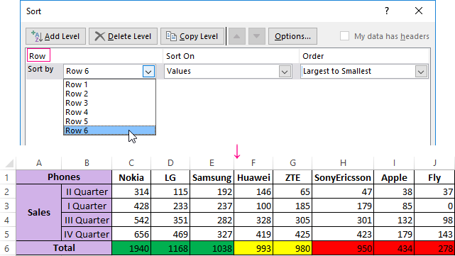
- Right-click on the table. Select «Sort» and method «Largest to Smallest».
- Open the «DATA» tab — «Sort» dialog box.
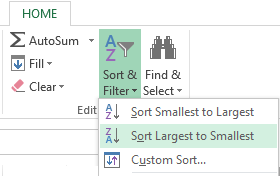
Frequently used sorting methods are represented by a single button on the «HOME» tab «Editing» section.
Sorting the table by a separate column:
- For the program to perform the task correctly, select the required column in the data range.
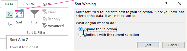
- Then we act in accordance with the task. If you want to perform simple sorting in ascending / descending order (alphabet or vice versa), just click the corresponding button on the taskbar. When the range contains more than one column, Excel opens a dialog box like:

To maintain the correspondence of the values in the lines, we select the action «Expand the selection». Otherwise, only the selected column is sorted — the structure of the table is broken.
If you select the entire table and sort it, the first column is sorted. Data in the rows will be in accordance with the position of the values in the first column.
Sorting by the cell color and font
Excel provides rich formatting capabilities to the user. Therefore, it is possible to operate in different formats.
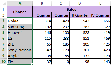
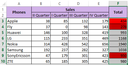
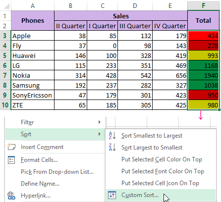
We will make the column «Total» and «fill» the cells with values in different shades in the training table. Perform the color sorting:
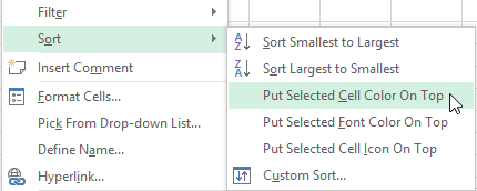
- Select the column — the right mouse button — «Sort».
- From the proposed list, select «Put Selected Cell Color On Top».
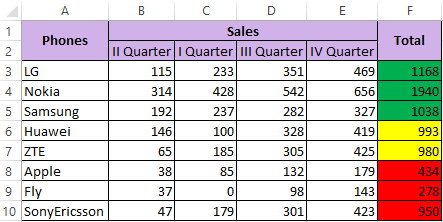
- We agree to «Expand the selection». Result:
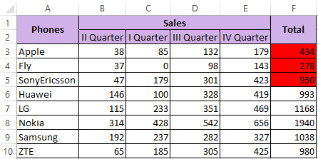
The program sorted cells by accents. The user can choose the order of the color sorting. For this purpose, in the list of tool options, select «Custom Sort».
In the window that opens, enter the required parameters:
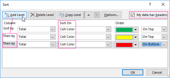
Here you can choose the order of the representation the cells of different colors.
By the same principle, the font data is sorted.
Sorting by multiple columns in Excel
How to set the order of secondary sorting in Excel? To solve this problem, you need to set several sorting conditions.
- Open the menu «Custom Sort». Assign the first criterion.
- Click the button «Add Level».
- There are windows for entering data for the next sorting condition. We fill them.
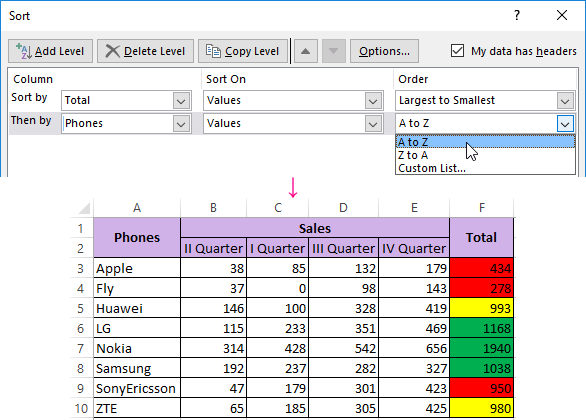
The program allows you to add several criteria at once to perform the sorting in a special order.
Sorting the rows in Excel
By default, the data is sorted by columns. How to sort by rows in Excel:
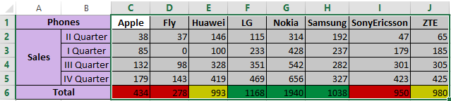
- In the «Custom Sort» dialog box, click the «Options» button.
- In the menu that opens, select «Range Columns».
- Click OK. In the «Sort» window, fields for filling in the conditions for the rows appear.

Thus, the table is sorted into Excel by several parameters.
Random sorting in Excel
The built-in sorting options do not allow you to arrange data in a column randomly. This task will be handled by the function =RAND().
For example, you need to arrange a set of certain numbers in a random order.
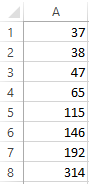
We put the cursor in the next cell (left-right, not important). In the formula row, enter =RAND(). Press Enter. We copy the formula to the whole column — we get a set of random numbers.
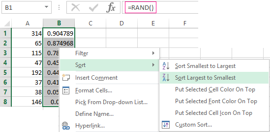
Now sort the resulting column in ascending / descending order — the values in the original range will automatically be placed in random order.
Dynamic table sorting in Excel
If you apply standard sorting to the table, then when you change the data, it will not be relevant. You need to make sure that the values are sorted automatically. We use formulas.
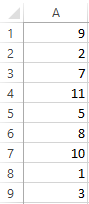
- There is a set of primes that need to be sorted in ascending order.
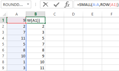
- Put the cursor in the next cell and enter the formula: =SMALL(A:A,ROW(A1)). Exactly, as a range we specify the whole column. And as a coefficient there is the function of SMALL() ROW() with reference to the first cell.
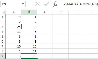
- Lets change the number in the initial range to 7 to 25 — «sorting» ascending will also change.
If it is necessary to make the dynamic sorting in descending order, use the =LARGE() function.
To sort the text values dynamically, you need the array formulas.
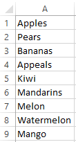
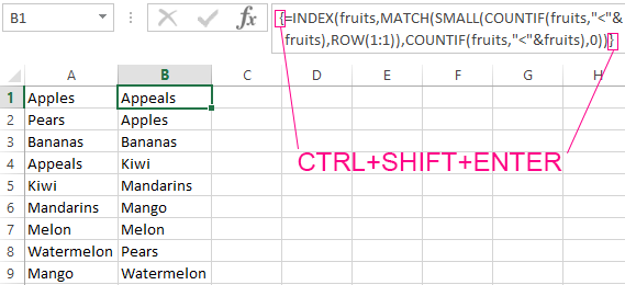
- Initial data is a list of some names in any order. In our example it is a list of fruits.
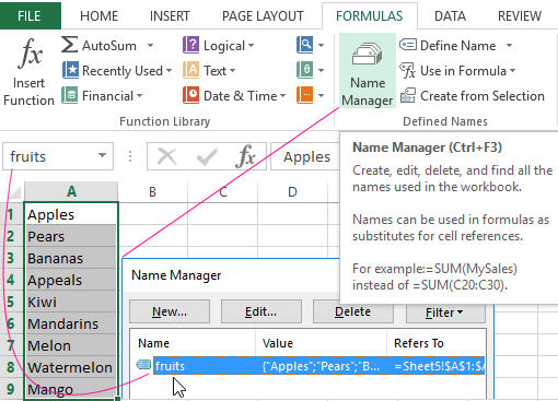
- Select the column and give it the name «fruits». To do this, in the field of names that is near the formula line, enter the name we need to assign it to the selected range of cells.
- In the next cell (in the example — in B1), we write the formula:
Since we have an array formula before us, press Ctrl + Shift + Enter. We multiply the formula by the whole column.
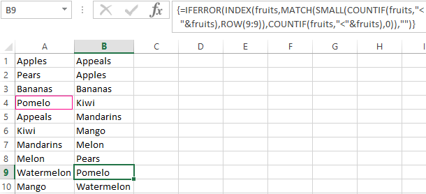
- If lines are added to the original column, then we introduce a slightly modified formula:
Add the «pomelo» value to the «fruit» name range and check:
Download sorting data in excel using formulas
Subsequently, when you add data to the table, the sorting process will be performed automatically.
We can use array formulas to get the average of each column and row in Excel 365.
No need to depend on AVERAGE() based non-array formulas, which require drag-down/right.
Then what are the alternative solutions?
We can use the two other alternatives to calculate the average in Excel 365. They are SUBTOTAL and AGGREGATE.
We can use the former function for our purpose.
You May Like: Differences Between SUBTOTAL and AGGREGATE Functions in Excel.
You may use the following syntaxes of the dynamic array formulas to get the average of each column and row in Excel 365.
Syntax # 1: Average of Each Column:
=SUBTOTAL(1,OFFSET(columns))Syntax # 2: Average of Each Row:
=SUBTOTAL(1,OFFSET(rows))In addition to the SUBTOTAL, we will use the OFFSET function. It will dynamically offset rows/columns.
Sample Data to Average Each Column and Row in Excel 365
I have recorded the sales of three items from July to December, i.e., the last six months in a year.
The goal is to get the average of the sales made:
1. For each item over the last six months (average by the column).
2. For each month across all items (average by the row).

Usually, we may enter the following non-array formula in cell F3 and drag-down to average each row in Excel.
=AVERAGE(B3:D3)To average each column in Excel, we may use the following formula in cell B10 and darg-right.
Let’s see how to materialize this in Excel 365 with array formulas.
Steps
Please follow the below steps.
Array Formula to Average Each Column in Excel 365
1. Empty B10:D10 for the formula to spill the result.
2. Insert the below SUBTOTAL formula in cell B10, which will return the average of “Item 1” for the last six months.
=SUBTOTAL(1,B3:B8)3. We should make it expand to its right. For that, we can follow syntax # 1 above (please scroll up to see the syntax).
As per that syntax, you may replace B3:B8 with OFFSET(columns)which is equal to;
OFFSET(B3,,SEQUENCE(1,COLUMNS(B3:D3),0),ROWS(A3:A8))4. Based on it, here is the code to average each column in Excel 365.
=SUBTOTAL(1,OFFSET(B3,,SEQUENCE(1,COLUMNS(B3:D3),0),ROWS(A3:A8)))Anatomy of the OFFSET(columns)
It’s equal to OFFSET(offset_starting_from,,number_of_columns_to_offset,height)
offset_starting_from = B3

number_of_columns_to_offset = SEQUENCE(1,COLUMNS(B3:D3),0)– It is equal to =SEQUENCE(1,3,0) which returns the sequence {0, 1, 2} (horizontally).
It’s the key!
The SEQUENCE helps the OFFSET to dynamically offset columns, i.e., 0 – first column, 1 – the second column, and 2 – the third column.
height = ROWS(A3:A8)– It’s the height of the range that is six rows.
Related: Reverse Sequence in Excel 365 – Formula and Examples.
Array Formula to Average Each Row in Excel 365
1. Empty F3:F8 for the formula to spill the result.
2. Insert the below SUBTOTAL formula in cell F3, which will return the average of all the items for July.
=SUBTOTAL(1,B3:D3)3. We should make it expand down. For that, we can follow syntax # 2 above (please scroll up to see the syntax).
As per that syntax, you may replace B3:D3 with OFFSET(rows), which is equal to;
OFFSET(B3,SEQUENCE(ROWS(A3:A8),1,0),,,COLUMNS(B2:D2))4. Based on it, here is the code to average each row in Excel 365.
=SUBTOTAL(1,OFFSET(B3,SEQUENCE(ROWS(A3:A8),1,0),,,COLUMNS(B2:D2)))Anatomy of the OFFSET(rows)
It’s equal to OFFSET(offset_starting_from,,number_of_rows_to_offset,width)
offset_starting_from = B3
number_of_rows_to_offset = SEQUENCE(ROWS(A3:A8),1,0)– It is equal to =SEQUENCE(6,1,0) which returns the sequence {0; 1; 2; 3; 4; 5} (vertically).
It’s the key formula here!
The SEQUENCE helps the OFFSET to dynamically offset rows, i.e., 0 – the first row, 1 – the second row, 3 – the third row, and so on.
width = COLUMNS(B2:D2)– It’s the width of the range that is three columns.
Resources
- Find the Largest Value in Each Row or Column in Excel 365.
- Find the Smallest Value in Each Row or Column in Excel 365.
- Spill Formulas to Sum Each Row in Excel 365.
- How to Retrieve the Last Record in Each Group in Excel 365.
- XLOOKUP Nth Occurrence in Excel (First, Last, and Nth).
- How to Use Wildcards in Filter Function in Excel (Alternatives).
- Gantt Chart Formula in Excel 365 (Conditional Coloring).
Return to Excel Formulas List
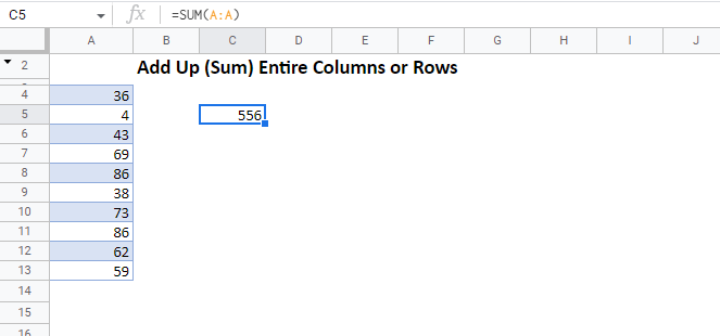
This tutorial demonstrates how to add entire rows or columns in Excel.
The Sum Function
We will use the Sum Function to add up entire rows and columns. It takes input in two primary forms:
- Standalone Cell References =sum(a1,b2,c3)
- Arrays of Cells =sum(A1:E1).
We will use the latter method to sum range A1 to E1:
=SUM(A1:E1)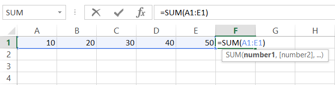
Tip 1: The shortcut ALT + = (press and hold ALT then tap =) will automatically create a Sum Function. When possible, Excel will guess which cells you would like to sum together, populating the Sum Function.
Tip 2: After using the ALT + = shortcut or after typing =sum(, use the arrow keys to select the appropriate cell. Then hold down SHIFT or CTRL + SHIFT to select the desired range of cells.
Tip 3: Instead of using the keyboard, you can also use the mouse to drag and highlight the desired range and complete the formula.
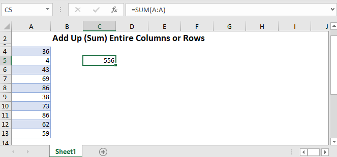
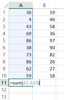
Sum an Entire Column
To add up an entire column, enter the Sum Function: =sum( and then enter the desired column. There are several ways to do this:
- Type the columns “A:A”
- Click the column letter at the top of the worksheet
- Use the arrow keys to navigate to the column and using the CTRL + SPACE shortcut to select the entire column.
The formula will be in the form of.
=sum(A:A)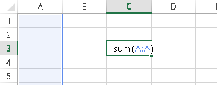
Sum an Entire Row
To sum an entire row, use the same method as with columns:
- Type the rows “3:3”
- Click the row number at the left of the worksheet
- Use the arrow keys to navigate to the column and using the SHIFT + SPACE shortcut to select the entire row.
The formula will be in the form of.
=sum(1:1)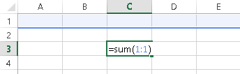
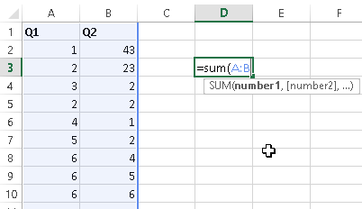
Add up Multiple Columns or Rows at Once
To sum columns or rows at the same time, use a formula of the form: =sum(A:B) or =sum(1:2). Remember that you can also use the keyboard shortcuts CTRL + SPACE to select an entire column or SHIFT + SPACE an entire row. Then, while holding down SHIFT, use the arrow keys to select multiple rows.
Sum Non-Contiguous Columns or Rows at Once
To sum Non-Contiguous Columns or Rows at Once, enter the separate ranges (columns or rows) separated by commas:
=SUM(A:A,B:B)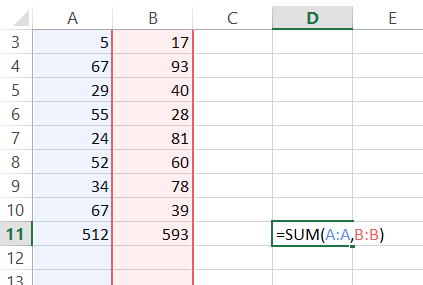
Sum Everything Except the Header
You may need to add up an entire column (or row), except the header. Non-numerical values will be automatically excluded, but if the header is numeric, the pervious methods will not work well
Instead, you can use a formula like this
=SUM(A2:A1048576)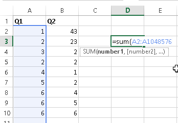
Why 1,048,576? Excel worksheets only have 1,048,576 rows!
To see how many rows Excel has, select a cell in a blank column then you use the shortcut: CTRL + Down Arrow to navigate to the last row in the worksheet.
Sum to End of Column
Instead of adding up an entire column to the bottom of the worksheet, you can add-up only the rows containing data. To do this, first start your SUM Function. Then select the first row in the column containing the data you wish to sum, then use CTRL + SHIFT + Down Arrow to select all the cells in that column (Note: be careful of blank cells. CTRL + SHIFT + Arrow will navigate to the cell directly before a blank cell)
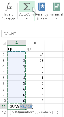
AutoSum Magic
Select a cell above/below or left/right the range you want to sum. Then use the shortcut ALT + = or select the Formulas Ribbon > AutoSum. Doing so will automatically generate a formula for you!
Common Sum Errors
#VALUE! – you have non-integers in the sum formula (not an issue in Excel 2013+)
#REF! – previously referenced column(s) or row(s) does not exist anymore
#NAME? – check formula spelling
For more information about Autosum in Excel visit Microsoft’s Website
Sum Entire Rows or Columns in Google Sheets
All the examples work the same in Google Sheets as Excel, except (annoyingly) you can not use the keyboard shortcuts to select entire rows or columns.