
If the first row (row 1) or column (column A) is not displayed in the worksheet, it is a little tricky to unhide it because there is no easy way to select that row or column. You can select the entire worksheet, and then unhide rows or columns (Home tab, Cells group, Format button, Hide & Unhide command), but that displays all hidden rows and columns in your worksheet, which you may not want to do. Instead, you can use the Name box or the Go To command to select the first row and column.
-
To select the first hidden row or column on the worksheet, do one of the following:
-
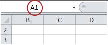
In the Name Box next to the formula bar, type A1, and then press ENTER.

-
On the Home tab, in the Editing group, click Find & Select, and then click Go To. In the Reference box, type A1, and then click OK.
-
-
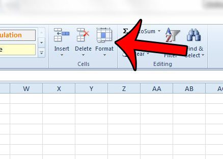
On the Home tab, in the Cells group, click Format.
-
Do one of the following:
-
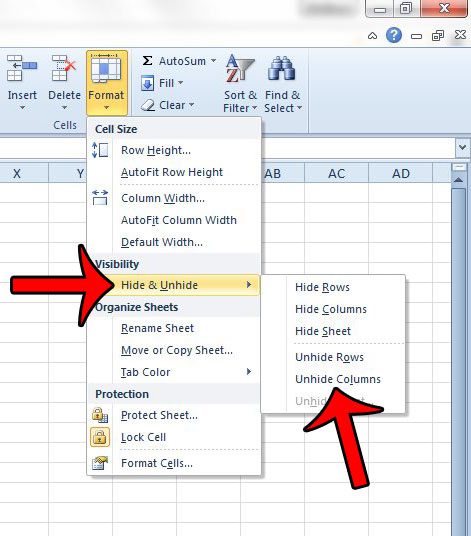
Under Visibility, click Hide & Unhide, and then click Unhide Rows or Unhide Columns.
-
Under Cell Size, click Row Height or Column Width, and then in the Row Height or Column Width box, type the value that you want to use for the row height or column width.
Tip: The default height for rows is 15, and the default width for columns is 8.43.
-
If you don’t see the first column (column A) or row (row 1) in your worksheet, it might be hidden. Here’s how to unhide it. In this picture column A and row 1 are hidden.
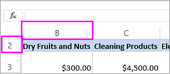
To unhide column A, right-click the column B header or label and pick Unhide Columns.
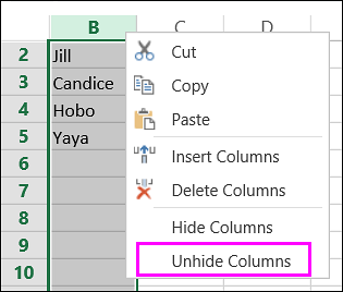
To unhide row 1, right-click the row 2 header or label and pick Unhide Rows.
Tip: If you don’t see Unhide Columns or Unhide Rows, make sure you’re right-clicking inside the column or row label.
Unhiding the first column, or column “A” in an Excel spreadsheet presents a unique challenge. The typical method for unhiding a column will not apply when the column that is hidden is the leftmost one in the worksheet. An alternative would be to simply unhide all of the columns that are hidden in the spreadsheet, but this can be problematic if there are other columns that you wish to remain hidden.
Fortunately it is possible to unhide only the first column in your spreadsheet by following the procedure outlined below.
Unhiding the First Column in Excel 2010
The steps in this article will assume that you have hidden the first column in your Excel spreadsheet. The procedure below will only unhide column “A”. If there are other hidden columns, they will remain hidden. If you wish to unhide all of the hidden columns in your spreadsheet, then you can follow the steps here.
Step 1: Open your spreadsheet in Excel 2010.
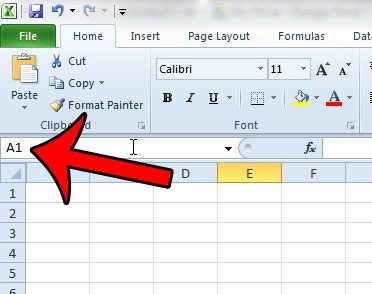
Step 2: Click inside the Name field at the top-left of the spreadsheet.
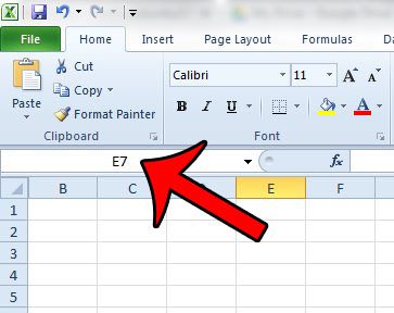
Step 3: Type “A1” into this field, then press the Enter key on your keyboard.
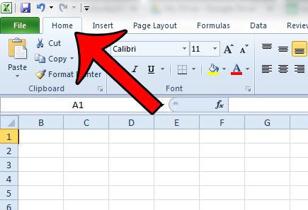
Step 4: Click the Home tab at the top of the window.
Step 5: Click the Format button in the Cells section of the Office ribbon.
Step 6: Click the Hide & Unhide option, then click Unhide Columns.
Column “A” should now be visible in your spreadsheet. If you are still unable to see the first column of the worksheet, then it may not actually be hidden. You may want to consider unfreezing the panes in your worksheet, or removing a split screen. Both of these settings can often make it appear that a row or column is hidden when it is simply off screen.
Note that this same method will also work to unhide the first row of your spreadsheet, except you will need to select the Unhide Rows option in Step 6 instead.

Matthew Burleigh has been writing tech tutorials since 2008. His writing has appeared on dozens of different websites and been read over 50 million times.
After receiving his Bachelor’s and Master’s degrees in Computer Science he spent several years working in IT management for small businesses. However, he now works full time writing content online and creating websites.
His main writing topics include iPhones, Microsoft Office, Google Apps, Android, and Photoshop, but he has also written about many other tech topics as well.
Read his full bio here.
Watch Video – How to Unhide Columns in Excel
If you prefer written instruction instead, below is the tutorial.
Hidden rows and columns can be quite irritating at times.
Especially if someone else has hidden these and you forget to unhide it (or even worse, you don’t know how to unhide these).
While I can’t do anything about the first issue, I can show you how to unhide columns in Excel (the same techniques can also be used to unhide rows).
It may happen that one of the methods of unhiding columns/rows may not work for you. In that case, it is good to know the alternatives that can work.
There are many different situations where you may need to unhide the columns:
- Multiple columns are hidden and you want to unhide all columns at once
- You want to unhide a specific column (in between two columns)
- You want to unhide the first column
Let’s go through each for these scenarios and see how to unhide the columns.
Unhide All Columns At One Go
If you have a worksheet that has multiple hidden columns, you don’t need to go hunt each one and bring it to light.
You can do that all in one go.
And there are multiple ways to do this.
Using the Format Option
Here are the steps to unhide all columns at one go:
- Click on the small triangle at the top left of the worksheet area. This will select all the cells in the worksheet.
- Right-click anywhere in the worksheet area.
- Click on Unhide.
No matter where that pesky column is hidden, this will unhide it.
Note: You can also use the keyboard shortcut Control A A (hold the control key and hit the A key twice) to select all the cells in the worksheet.
Using VBA
If you need to do this often, you can also use VBA to get this done.
The below code will unhide column in the worksheet.
Sub UnhideColumns ()
Cells.EntireColumn.Hidden = False
EndSub
You need to place this code in the VB Editor (in a module).
If you want to learn how to do this with VBA, read a detailed guide on how to run a macro in Excel.
Note: To save time, you can save this macro in the Personal Macro Workbook and add it to the quick access toolbar. This will allow you to unhide all columns with a single click.
Using a Keyboard Shortcut
If you’re more comfortable using keyboard shortcuts, there is a way to unhide all columns with a few keystrokes.
Here are the steps:
- Select any cell in the worksheet.
- Press Control-A-A (hold the control key and press A twice). This will select all the cells in the worksheet
- Use the following shortcut – ALT H O U L (one key at a time)
If you can get hang of this keyboard shortcut, it could be a lot faster to unhide columns.
Note: The reason you need to press A twice when holding the control key is that sometimes when you press Control A, it only selects the used range in Excel (or the area that has the data) and you need to press the A again to select the entire worksheet.
Another keyword shortcut that works for some and not for others is Control 0 (from a numeric keypad) or Control Shift 0 from a non-numeric keypad. It used to work for me earlier but doesn’t work anymore. Here is some discussion on why it may happen. I suggest you use the longer (ALT HOUL) shortcut that works every time.
Unhide Columns in Between Selected Columns
There are multiple ways you can quickly unhide columns in between selected columns. The methods shown here are useful when you want to unhide a specific column(s).
Let’s go through these one-by-one (and you can choose to use that you find the best).
Using a Keyboard Shortcut
Below are the steps:
- Select the columns that contain the hidden columns in between. For example, if you are trying to unhide column C, then select column B and D.

- Use the following shortcut – ALT H O U L (one key at a time)

This will instantly unhide the columns.
Using the Mouse
One quick and easy way to unhide a column is to use the mouse.
Below are the steps:
Using the Format Option in the Ribbon
Under the home tab in the ribbon, there are options to hide and unhide columns in Excel.
Here is how to use it:
Another way of accessing this option is by selecting the columns and right clicking using the mouse. In the menu that appears, select the unhide option.

Using VBA
Below is the code that you can use to unhide columns in between the selected columns.
Sub UnhideAllColumns()
Selection.EntireColumn.Hidden = False
End Sub
You need to place this code in the VB Editor (in a module).
If you want to learn how to do this with VBA, read a detailed guide on how to run a macro in Excel.
Note: To save time, you can save this macro in the Personal Macro Workbook and add it to the quick access toolbar. This will allow you to unhide all columns with a single click.
By Changing the Column Width
There is a possibility that none of these methods work when you try to unhide column in Excel. It happens when you change the Column Width to 0. In that case, even if you unhide the column, it’s width still remains 0, and hence you can’t see it or select it.
Below are the steps to change the column width:
This is by far the most reliable way to unhide columns in Excel. If everything fails, just change the column width.
Unhide the First Column
Unhiding the first column can be a little bit tricky.
You can use many of the methods covered above, with a little bit of extra work.
Let me show you a few ways.
Use the Mouse to Drag the First Column
Even when the first column is hidden, Excel allows you to select it and drag it to make it visible.
To do this, hover the cursor on the left edge of column B (or whatever is the leftmost visible column).
The cursor would change into a double arrow pointer as shown below.

Hold the left mouse button and drag the cursor to the right. You will see that it unhides the hidden column.

Go to a Cell in the First Column and Unhide it
But how do you go to any cell in the column that’s hidden?
Good question!
You use the Name Box (it’s left to the formula bar).

Enter A1 in the Name Box. It will instantly take you to the A1 cell. Since the first column is hidden, you won’t be able to see it, but be assured that it’s selected (you’ll still see a thin line just left of B1).
Once the hidden column cell is selected, follow the below steps:
- Click the Home tab.
- In the Cells group, click on Format.
- Hover the cursor on the ‘Hide & Unhide’ option.
- Click on ‘Unhide Columns’
Select the First Column and Unhide it
Again! How do you select it when it’s hidden?
Well, there are many different ways to skin the cat.
And this is just another method in my kitty (this is the last cat sounding reference I promise).
When you select the leftmost visible cell and drag the cursor to the left (where there are row numbers), you end up selecting all the hidden columns (even when you don’t see it).

Once you have select all the hidden columns, follow the below steps:
- Click the Home tab.
- In the Cells group, click on Format.
- Hover the cursor on the ‘Hide & Unhide’ option.
- Click on ‘Unhide Columns’
Check The Number of Hidden Columns
Excel has an ‘Inspect Document’ feature that is meant to quickly scan the workbook and give you some details about it.
And one of the things that you can do that ‘Inspect Document’ is to quickly check how many hidden columns or hidden rows are there in the workbook.
This might be useful when you get the workbook from someone and want to quickly inspect it.
Below are the steps on how to check the total number of hidden columns or hidden rows:
- Open the workbook
- Click on the File tab
- In the Info options, click on the ‘Check for Issues’ button (it’s next to the Inspect Workbook text).

- Click on Inspect Document.

- In the Document Inspector, make sure Hidden Rows and Columns option is checked.

- Click the Inspect button.
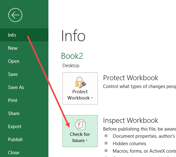


This will show you the total number of hidden rows and columns.

It also gives you the option to delete all these hidden rows/columns. This can be the case if there is extra data that has been hidden and is not needed. Instead of finding hidden rows and columns, you can quickly delete these from this option.
You May Also Like the following Excel Tips/Tutorials:
- How to Insert Multiple Rows in Excel – 4 Methods.
- How to Quickly Insert New Cells in Excel.
- Keyboard & Mouse Tricks that will Reinvent the Way You Excel.
- How to Hide a Worksheet in Excel.
- How to Unhide Sheets in Excel (All In One Go)
- Excel Text to Columns (7 Amazing things you can do with it)
- How to Lock Cells in Excel
- How to Lock Formulas in Excel
Posted by Mikko Peltoniemi 2012-08-09T14:44:13Z
In an Excel file, I have column A, that’s as if its width is set to 0. But it’s not, I’ve tried setting the Column Width to various values with no success.
If I select B1, and go left, I can see the value in A1, so the column is not hidden either.
I can see the column in Print Preview. I just can’t view it.
What happened to it?

1 Reply
-
Ok, got it as soon as I posted… Unfreeze Panes did the trick.
lock
This topic has been locked by an administrator and is no longer open for commenting.
To continue this discussion, please ask a new question.
Read these next…
Snap! — Rollerblading Robot, Cyborg Cockroaches, AI Pi, 20-foot Donkey Kong
Spiceworks Originals
Your daily dose of tech news, in brief.
Welcome to the Snap!
Flashback: April 13, 2000: Metallica Sues Napster (Read more HERE.)
Bonus Flashback: April 13, 1970: Oxygen Tank on Apollo 13 Explodes (Read more HERE.)
You need to hear this…
Spark! Pro series — 13th April 2023
Spiceworks Originals
Today in History: Fans toss candy bars onto baseball field during MLB gameOn April 13, 1978, opening day at Yankee Stadium, the New York Yankees give away thousands of Reggie! bars to fans, who naturally toss them onto the field after star outfielder …
Remote worker content filtering
Security
GreetingsI am in the process of looking for a product to help protect and monitor employee network traffic. My biggest hurdle is that 75% of my employees all work from home. Does anyone have any suggestions for products that would monitor web traffic and …
Salary Negotiations?
IT & Tech Careers
SpiceHeads,If you get a offer from a company and sign off on it and during the onboard process background checks , drug test etc.You get another offer for more money can you go back to the 1 st offer of the job you really want and ask for more or how woul…
IT Adventures: Episode Three — Danger
Holidays
Tell a Story day is coming up on April 27th, and were working on an interactive story for it. Here’s the idea. Below, there will be a story prompt which is sort of like a Choose Your Own Adventure, except that the rest of it isn’t written. …


Why Are The Columns/Rows Missing?
If you landed on this article, you’ve probably been pulling your hair out trying to figure out why you can’t unhide your Excel spreadsheet rows or columns. They just appear to be missing!
This is not a glitch or bug within your Excel file, it’s actually an intended spreadsheet feature (when used correctly). The feature that is causing this is Excel’s Freeze Panes button.
Why Is This Happening?
When you apply Freeze Panes to your spreadsheet, it essentially locks the view based on where the window is scrolled to. This means that if there are rows/columns that are not visible to either the left or top of your spreadsheet, these cells will remain unviewable once Freeze Panes has been activated. This essentially prevents you from accessing (unhiding) them.
An alternate scenario where this will occur is when Row 1 is part of an outline group and is collapsed prior to the Freeze Pane being applied. Oddly enough, this does not occur is Column A is part of a collapsed group as you can freely expand/collapse the group after the Freeze Pane has been applied.
Steps To Access/Fix The Locked Rows Or Columns
-
Go to the View tab in your Excel Ribbon
-
Click the Freeze Panes menu button within the Windows button group
-
Select the Unfreeze Panes button
Now you should be able to access those “missing” rows or columns.
Why Is Hiding With Freeze Panes Useful?
Locking (hiding) rows or columns with the freeze panes button can be a passive-aggressive way to keep others from vital formulas you don’t want messed with. If you don’t want to deal with setting and remembering passwords, this can be a great alternative to preventing your users from easily accessing sections of your spreadsheet.
Hidings Rows or Columns With Freeze Panes
If you would like to hide or lock yourself from being able to access rows in the top portion or columns on the left side of your spreadsheet, you simply need to do the following:
-
Scroll horizontally and vertically to position any rows/columns you wish to hide so they do not appear on your screen
-
Select the cell you wish to designate for your Freeze Panes application
-
Navigate to the View Tab and enable your Freeze Panes
After you have completed these steps, you will be unable to access the rows or columns you locked from view until your click the Unfreeze Panes button.
Hiding Grouped Rows With Freeze Panes
If you would like to hide or lock yourself from being able to access an outline grouping of rows in the top portion of your spreadsheet, you simply need to do the following:
-
Apply your outline grouping to the rows you wish to collapse
-
IMPORTANT! In order for this to work, Row 1 must be part of your grouping. If it is not, you will still be able to expand the outline group when the Freeze Panes are applied.
-
-
Select the cell you wish to designate for your Freeze Panes application
-
Navigate to the View Tab and enable your Freeze Panes
After you have completed these steps, you will be unable to access the collapsed rows until your click the Unfreeze Panes button.
I Hope This Helped!
Hopefully, I was able to explain how you can unlock or lock rows/columns in your spreadsheet using the Freeze Panes feature. If you have any questions about this technique or suggestions on how to improve it, please let me know in the comments section below.
About The Author
Hey there! I’m Chris and I run TheSpreadsheetGuru website in my spare time. By day, I’m actually a finance professional who relies on Microsoft Excel quite heavily in the corporate world. I love taking the things I learn in the “real world” and sharing them with everyone here on this site so that you too can become a spreadsheet guru at your company.
Through my years in the corporate world, I’ve been able to pick up on opportunities to make working with Excel better and have built a variety of Excel add-ins, from inserting tickmark symbols to automating copy/pasting from Excel to PowerPoint. If you’d like to keep up to date with the latest Excel news and directly get emailed the most meaningful Excel tips I’ve learned over the years, you can sign up for my free newsletters. I hope I was able to provide you with some value today and I hope to see you back here soon!
— Chris
![]()
Download Article
Quickly display one or more hidden columns in your Excel spreadsheet
![]()
Download Article
- Using the Column Drag Tool
- Using Right Click
- Unhiding One Column with the Name Box
- Unhiding All Columns
- Q&A
- Tips
|
|
|
|
|
Are you having trouble viewing certain columns in your Excel workbook? This wikiHow guide shows you how to display a hidden column in Microsoft Excel. You can do this on both the Windows and Mac versions of Excel. There are multiple simple methods to unhide hidden columns. You can drag the columns, use the right-click menu, or format the columns.
Things You Should Know
- Hover your cursor to the right of the hidden columns, then click and drag to the right to unhide them.
- Alternatively, select the columns adjacent to the hidden columns. Then right-click and select Unhide.
- You can also go to Home > Format > Hide & Unhide to show hidden columns.
-
1
Hover your cursor directly to the right of the hidden columns. When your cursor is between the column letters adjacent to the hidden columns, the cursor will change into two parallel lines with two arrows pointing horizontally.
- You can identify hidden columns by looking for two lines between column letters.
- Your cursor needs to be to the right of the two lines for this method. Placing the cursor to the left will increase the column size of the left adjacent column.
-
2
Click and drag to the right. This will unhide the hidden columns between the adjacent columns.
- Alternatively, you can double-click to immediately unhide the hidden column.
Advertisement
-
3


Advertisement
-
1
Select the columns on both sides of the hidden columns. To do this:
- Hold down the ⇧ Shift key while you click both letters above the column
- Click the left column next to the hidden columns.
- Click the right column next to the hidden columns.
- The columns will be highlighted when you successfully select them.
- For example, if column B is hidden, you should click A and then C while holding down ⇧ Shift.
-
2
Right-click either of the selected columns. This will open the right-click pop up menu.
-
3
Select Unhide in the right-click menu. The hidden columns between the two selected columns will be unhidden.
- For more helpful excel tricks, check out our intro guide to Excel.


Advertisement
-
1
Click the Name Box. This is the drop down box to the left of the formula box.[1]
- This method is great for unhiding the first column (A) since there isn’t a column to its left that you can select to access the right-click Unhide menu option.
-
2
Type A1 in the Name Box and press ↵ Enter. Replace A with the letter of the column you want to unhide.
-
3
Click the Home tab. It’s in the upper-left corner of the Excel window.
-
4
Click Find & Select. This is in the «Editing» group in the Home tab. A drop down menu will open.
-
5
Select Go To. This will open the «Go To» window.
-
6
Type A1 in the «Reference» box and click OK.
-
7
Click the Home tab. It’s in the upper-left corner of the Excel window.
-
8
Click Format. This button is in the «Cells» section of the Home tab; you’ll find this section on the right side of the toolbar. A drop down menu will appear.[2]
-
9
Select Hide & Unhide. This option is below the «Visibility» heading in the Format drop down menu. Selecting it will open a pop up menu.
-
10
Click Unhide Columns. It’s near the bottom of the Hide & Unhide menu. Doing so will immediately unhide the column you selected in the Name Box.


Advertisement
-
1
Click the triangle in the top left corner of the spreadsheet. This is next to the row 1 label and column A label. Clicking the triangle will select the entire spreadsheet.
- Hiding columns can be useful for when you have data you don’t need at the moment, but want to keep in the spreadsheet. For example, if you’re tracking your bills in Excel, you might want to hide purchase categories when you’re only working with the sum totals.
-
2
Click the Home tab. It’s in the upper-left corner of the Excel window.
-
3
Click Format. This button is in the «Cells» section of the Home tab; you’ll find this section on the right side of the toolbar. A drop down menu will appear.
-
4
Select Hide & Unhide. This option is below the «Visibility» heading in the Format drop down menu. Selecting it will open a pop up menu.
-
5
Click Unhide Columns. It’s near the bottom of the Hide & Unhide menu. Doing so will immediately unhide every hidden column in the sheet.


Advertisement
Add New Question
-
Question
What do I do if the hidden columns are A and B?

You can select the whole document and do the steps above to retrieve all hidden columns.
-
Question
What do I do if I’ve followed the instructions provided, but I still cannot unhide column A in Excel?
Try unfreezing the column and unhiding, or freezing then unfreezing then unhiding. This process will work.
-
Question
If column A is hidden in excel, how do I find it?
Just use the search bar on top and type there «A1» the hidden column should appear.
See more answers
Ask a Question
200 characters left
Include your email address to get a message when this question is answered.
Submit
Advertisement
-
If some columns are still not visible after you’ve attempted to unhide the columns, the width of the columns may be set to «0» or another small value. To widen the column, position your cursor on the right border of the column, and drag the column to increase its width.
-
If you want to unhide all hidden columns on an Excel spreadsheet, click on the «Select All» button, which is the blank rectangle to the left of column «A» and above row «1.» You can then proceed with the remaining steps in this article to unhide those columns.
Thanks for submitting a tip for review!
Advertisement
About This Article
Article SummaryX
1. Open your Excel document.
2. Select the columns on both sides of the hidden column.
3. Click Home
4. Click Format
5. Select Hide & Unhide
6. Click Unhide Columns
Did this summary help you?
Thanks to all authors for creating a page that has been read 666,342 times.
Is this article up to date?
Over the course of a long night, you prepared your spreadsheet. However, when you looked at it the next morning, you find that you cannot see several columns. Do not worry — Excel did not spontaneously erase data from your spreadsheet. It just means that you accidentally used the «Hide» feature on the missing columns. Fortunately, you can use the «Unhide» command to make individual or all hidden columns visible again.
Individual Columns
-
Open your Excel spreadsheet.
-
Select both columns on either side of the hidden column. To select the columns, place your cursor in the first column, drag it into the second column while holding down the mouse button and then drag the cursor down the second row. This will select both the visible and hidden columns.
-
Click «Format» in the Cells group of the Home tab.
-
Select «Visibility» followed by «Hide & Unhide» and «Unhide Columns» to make the missing column visible.
-
Repeat for the other missing columns in the spreadsheet.
All Hidden Rows
-
Open your Excel spreadsheet.
-
Click the «Select All» button, which is the button in the top left corner of the spreadsheet. You can also click «Ctrl-A» to select the entire spreadsheet.
-
Click «Format» in the Cells group of the Home tab.
-
Select «Visibility,» and then select «Hide & Unhide» and «Unhide Columns» to make all missing columns visible.
7 Methods to Unhide Columns in Excel
By hiding the data, the selected columns disappear from the display. However, the labels of the remaining columns stay the same. In addition, a thick bar in the column header area appears to indicate the hidden columns.
It is essential to know the techniques to unhide data. The seven ways to unhide Excel columns are stated as follows:
You can download this Unhide Columns Excel Template here – Unhide Columns Excel Template
- Home tab of Excel ribbon
- Shortcut key
- Context menu
- Column width
- Ctrl+G (go to) command
- Ctrl+F (find) command
- Double-line icon
Table of contents
- 7 Methods to Unhide Columns in Excel
- Unhide the First Column in Excel
- Locate and Unhide the Hidden Columns
- Create a Custom View
- Frequently Asked Questions
- Recommended Articles
In the given techniques, the method names followed by the steps to unhide are listed.
Method #1–Home Tab of Excel Ribbon
- Select the columns to the left and right of the hidden column.
- In the Home tab, under the “cells” group, click the “format” dropdown.
- From the “hide and unhide” option, select “unhide columns.”
Method #2–Shortcut Key
- Select the columns to the left and right of the hidden column.
- Press the shortcut “Alt H O U L.” Press one key at a time.
![]()
Method #3–Context Menu
- Select the columns to the left and right of the hidden column.
- Right-click on the selected columns and choose “unhide.”
Method #4–Column Width
- Select the columns to the left and right of the hidden column.
- Right-click on the selected columns and choose “column width.”
- Enter any number as the “column width.”
Method #5–Ctrl+G (Go To) Command
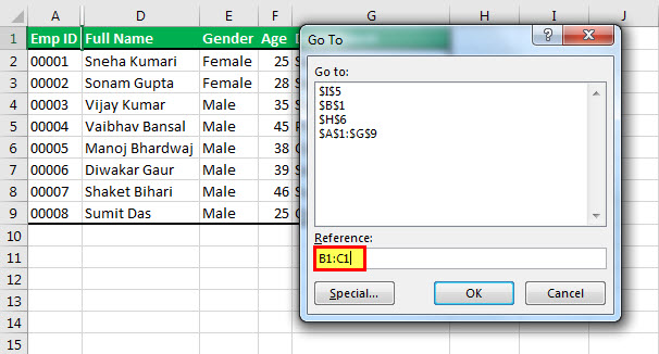
In the succeeding image, column B and C are hidden.
- In the Home tab, click “find and select” drop-down and choose “go to.” Alternatively, press the shortcut key F5.
- Specify any cell reference of the hidden column like B1:C1 in the “go to” dialog box. Click “Ok.”
- Choose any preceding technique (methods #1 to #4) to unhide columns B and C.
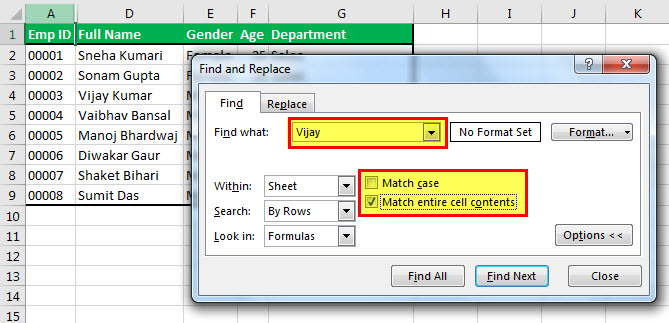
Method #6–Ctrl+F (Find) Command
In the succeeding image, column B and C are hidden.
- Press “Ctrl+F” and the “find and replace” dialog box appears.
- Enter the data of one of the hidden cells in the “find what” box.
- Click “options>>” and select the check box “match entire cell contents.”
- Click “find next” and close the “find and replace” dialog box.
- Select any preceding technique (methods #1 to #4) to unhide columns B and C.
Note: This method works in case the cell referenceCell reference in excel is referring the other cells to a cell to use its values or properties. For instance, if we have data in cell A2 and want to use that in cell A1, use =A2 in cell A1, and this will copy the A2 value in A1.read more is unknown and the cell data is known.
Method #7–Double-line Icon
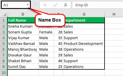
- Enter a single cell reference of the hidden column in the “name” box. This is the box to the left side of the formula bar.
- Press the “Enter” key.
- Select the columns to the left and right of the hidden column.
- Double-click the double-line icon (having arrows pointing to the left and right) in-between the column labels. Alternatively, follow method#1 to unhide the column.
Unhide the First Column in Excel
It is difficult to select and unhide the first column (column A). To unhide all the hidden columns in one go, follow method #1.
The steps to unhide only the first column are listed as follows:
- Type A1 in the name box (shown in the succeeding image) and press the “Enter” key. Alternatively, in the Home tab, click “find and select” drop-down and choose “go to.”
- In the Home tab, under the “cells” group, click the “format” dropdown.
- From the “hide and unhide” option, select “unhide columns.”
Locate and Unhide the Hidden Columns
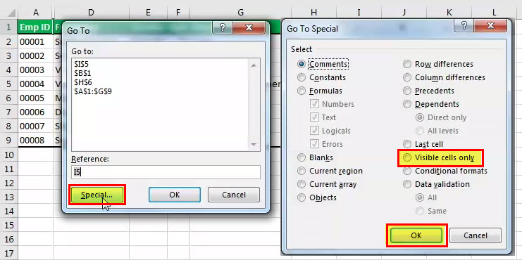
The steps to locate and unhide the hidden columns are listed as follows:
- Select the entire sheet.
- In the Home tab, click “find and select” drop-down and choose “go to.” Alternatively, click “go to special.”
- Click “special” and select the check box “visible cells only.” Click “Ok.”
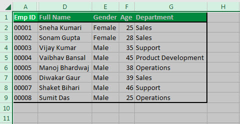
- The visible part of the table is highlighted (shown in the succeeding image). Moreover, a line between the column labels appears that shows the hidden columns.
- Select the highlighted part and follow any preceding technique (methods #1 to #4) to unhide columns B and C.
Create a Custom View
With the “custom view,” a user can save particular display settings. For instance, one user may want to hide columns while the other may wish to view the entire data in one go.
The steps to create a “custom view” are listed as follows:
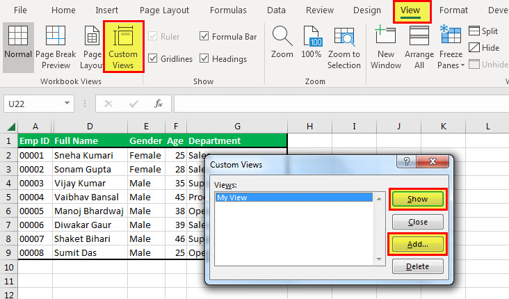
- In the View tab, click “custom views,” under the “workbook views” group.
- Click “add” and in the “add view” dialog box, enter a name for the view you want to create. The succeeding image shows the “custom view” titled “my view.”
- In “include in view,” select the settings of the view and click “Ok.”
- The “custom view” titled “my view” is created. Every time you select “my view” and click “show,” the display settings of “my view” become visible.
Hence, with the selection of “my view,” the columns A, D, E, F, and G are displayed, as shown in the succeeding image. The columns B and C are hidden because they were not active when “my view” was created.
Frequently Asked Questions
What does it mean to unhide columns in Excel?
Sometimes it becomes essential to hide particular columns to have a contracted view of the large data set. The option of hiding certain columns is better than deleting them. Before the spreadsheet containing hidden columns goes to the next user, it becomes essential to unhide them for facilitating a complete data view.
The steps to unhide the columns of the entire worksheet in one go are listed as follows:
• Select the entire worksheet by either clicking the triangle to the left of column A or pressing “Ctrl+A.”
• In the Home tab, under the “cells” group, click the “format” dropdown.
• From the “hide and unhide” option, select “unhide columns.”
Hence, all the columns of the worksheet become visible.
How to unhide the first column (column A) in Excel?
The three methods to unhide column A are listed as follows:
1. First method
a. Enter the reference A1 in the name box (to the left of the formula bar). Press the “Enter” key.
b. In the Home tab, under the “cells” group, click the “format” dropdown.
c. From the “hide and unhide” option, select “unhide columns.”
2. Second method
a. Select column B by clicking on its header.
b. Move the cursor to the left of column B till the double-line icon (having arrows pointing to the left and right) in the column header area appears.
c. Drag the double-line icon to the right for expanding column A.
3. Third method
a. In the Home tab, click “find and select” drop-down and choose “go to.” Alternatively, press the shortcut key F5.
b. In the “go to” dialog box, enter A1 in the “reference” box. Click “Ok” and the cell A1 is selected.
c. Follow the steps “b” and “c” of the first method.
How to unhide all Excel rows and columns with a shortcut key?
The steps to unhide all rows and columns with a shortcut key are listed as follows:
• Select the entire worksheet by either clicking the triangle to the left of column A or pressing “Ctrl+A.”
• Press the shortcut “Ctrl+Shift+9” to unhide all rows. Press all keys together.
• Select the entire worksheet again.
• Press the shortcut “Alt H O U L” to unhide all columns. Press one key at a time.
Recommended Articles
This has been a guide to unhide column in Excel. Here we discuss the Top 7 methods to unhide column in Excel along with examples. You may also look at these useful functions in Excel –
- Adding Columns in ExcelAdding a column in excel means inserting a new column to the existing dataset.read more
- Move Columns in ExcelMoving a column in excel means shifting the data of one column to another. It is similar to interchanging or swapping the data of two or more columns.read more
- VBA Delete ColumnIn VBA, deleting columns is simple. To select the column, we must first use the COLUMNS property, and then construct the syntax for the column delete method in VBA as follows: Columns (Column Reference). Deleteread more
- Excel Rows vs. ColumnsRows are combination of cells that are aligned horizontally, whereas columns are made up of cells that are aligned vertically. Rows are represented by numbers, whereas columns are represented by alphabets and alphabet combinations.read more
- Excel Date PickerExcel Date Picker is the drop-down calendar that facilitates the user to put the dates in the excel worksheet promptly. It is inserted with the help of ActiveX Control and is not available for the 64-bit version of MS Excel.read more