
Содержание
- Change the color or style of a chart in Office
- Change the color of a chart
- Change the chart style
- Change the appearance of your worksheet
- Change theme colors
- Change theme fonts
- Change theme effects
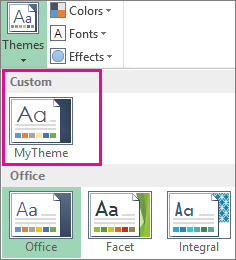
- Save a custom theme for reuse
- Use a custom theme as the default for new workbooks
- Change a theme and make it the default in Word or Excel
- I want to
- Choose a standard color theme
- Create my own color theme
- Change theme fonts
- Change theme effects
- Switch or remove a theme
- Save a custom theme for reuse
- Make my changes the new default theme
- Excel
- More about themes
- How to change the default colors that Excel uses for chart series
- To change the colors of the current workbook
- To make changes apply to all new workbooks
Change the color or style of a chart in Office
Maybe you’ve created a chart and think “this needs a little something else” to make it more impactful. Here’s where Chart Styles  is useful. Click the chart, click , located next to the chart in the upper right corner, and pick an option in the Style or Color galleries.
Change the color of a chart
Click the chart you want to change.
In the upper right corner, next to the chart, click Chart Styles .
Click Color and pick the color scheme you want.

Tip: Chart styles (combinations of formatting options and chart layouts) use the theme colors. To change color schemes, switch to a different theme. In Excel, click Page Layout, click the Colors button, and then pick the color scheme you want or create your own theme colors.
Change the chart style
Click the chart you want to change.
In the upper right corner next to the chart, click Chart Styles .
Click Style and pick the option you want.
As you scroll down the gallery, Live Preview shows you how your chart data will look with the currently selected style.
Источник
Change the appearance of your worksheet
To change the text fonts, colors, or general look of objects in all worksheets of your workbook quickly, try switching to another theme or customizing a theme to meet your needs. If you like a specific theme, you can make it the default for all new workbooks.
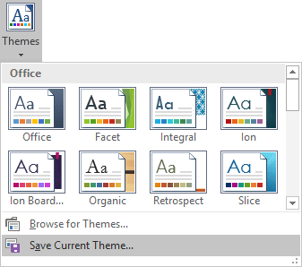
To switch to another theme, click Page Layout > Themes, and pick the one you want.
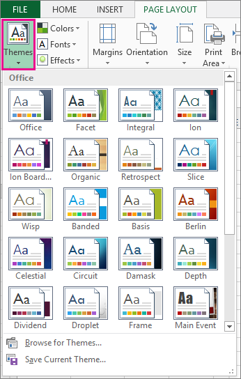
To customize that theme, you can change its colors, fonts, and effects as needed, save them with the current theme, and make it the default theme for all new workbooks if you want.
Change theme colors
Picking a different theme color palette or changing its colors will affect the available colors in the color picker and the colors you’ve used in your workbook.
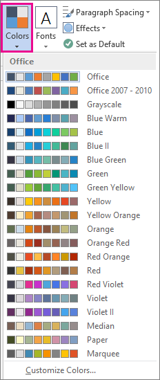
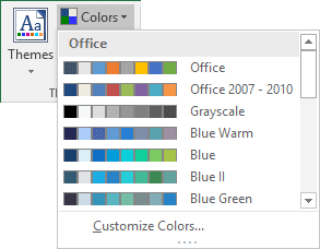
Click Page Layout > Colors, and pick the set of colors you want.
The first set of colors is used in the current theme.
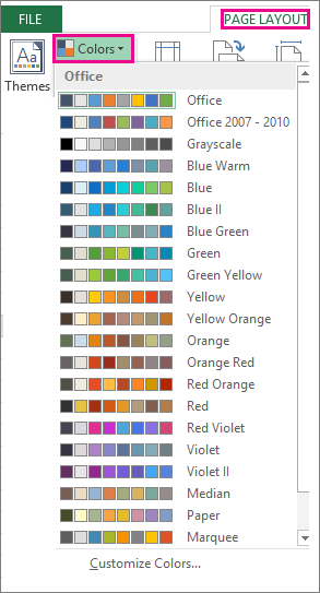
To create your own set of colors, click Customize Colors.
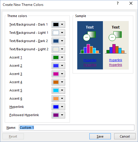
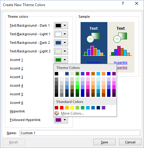
For each theme color you want to change, click the button next to that color, and pick a color under Theme Colors.
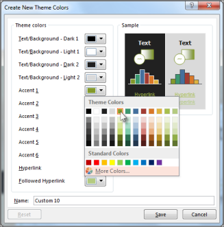
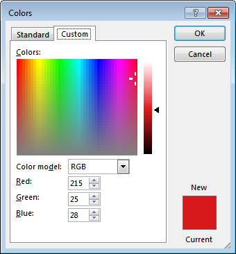
To add your own color, click More Colors, and then pick a color on the Standard tab or enter numbers on the Custom tab.
Tip: In the Sample box, you get a preview of the changes you made.
In the Name box, type a name for the new color set, and click Save.
Tip: You can click Reset before you click Save if you want to return to the original colors.
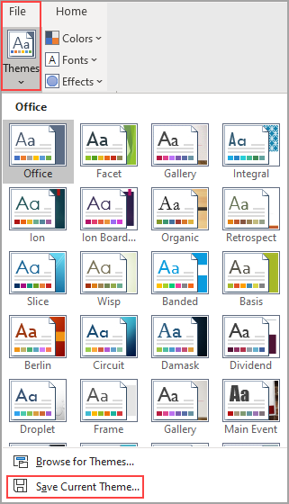
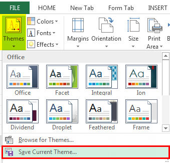
To save these new theme colors with the current theme, click Page Layout > Themes > Save Current Theme.
Change theme fonts
Picking a different theme font lets you change your text at once. For this to work, make sure Body and Heading fonts are used to format your text.
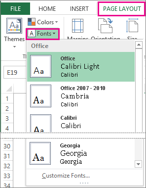
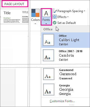
Click Page Layout > Fonts, and pick the set of fonts you want.
The first set of fonts is used in the current theme.
To create you own set of fonts, click Customize Fonts.
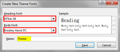
In the Create New Theme Fonts box, in the Heading font and Body font boxes, pick the fonts you want.
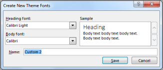
In the Name box, type a name for the new font set, and click Save.
To save these new theme fonts with the current theme, click Page Layout > Themes > Save Current Theme.
Change theme effects
Picking a different set of effects changes the look of the objects you used in your worksheet by applying different types of borders and visual effects like shading and shadows.
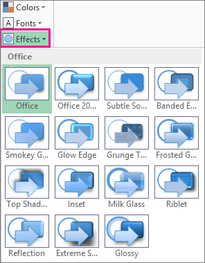
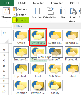
Click Page Layout > Effects, and pick the set of effects you want.
The first set of effects is used in the current theme.
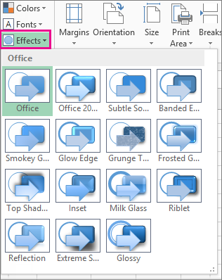
Note: You can’t customize a set of effects.
To save the effects you selected with the current theme, click Page Layout > Themes > Save Current Theme.
Save a custom theme for reuse
After making changes to your theme, you can save it to use it again.
Click Page Layout > Themes > Save Current Theme.
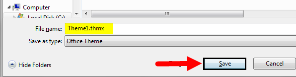
In the File name box, type a name for the theme, and click Save.
Note: The theme is saved as a theme file (.thmx) in the Document Themes folder on your local drive and is automatically added to the list of custom themes that appear when you click Themes.
Use a custom theme as the default for new workbooks
To use your custom theme for all new workbooks, apply it to a blank workbook and then save it as a template named Book.xltx in the XLStart folder (typically C:Users user nameAppDataLocalMicrosoftExcelXLStart).
To set up Excel so it automatically opens a new workbook that uses Book.xltx:
Click File> Options.
On the General tab, under Start up options, uncheck the Show the Start screen when this application starts box.
Источник
Change a theme and make it the default in Word or Excel
Document themes make it easy to coordinate colors, fonts, and graphic formatting effects across your Word, Excel, and PowerPoint documents and update them quickly. This video show you how-to change the entire theme, read below to just customize theme fonts, colors, or effects.

I want to
Choose a standard color theme
On the Page Layout tab in Excel or the Design tab in Word, click Colors, and pick the color set you want.
Tip: The first group of colors are the colors in the current theme.
Create my own color theme
On the Page Layout tab in Excel or the Design tab in Word, click Colors, and then click Customize Colors.
Click the button next to the theme color you want to change (for example, Accent 1 or Hyperlink), and then pick a color under Theme Colors.
To create your own color, click More Colors, and then pick a color on the Standard tab, or enter numbers or select a color on the Custom tab.
In the Sample pane, preview the changes that you made.
Repeat this for all the colors you want to change.
In the Name box, type a name for the new theme colors, and click Save.
Tip: To return to the original theme colors, click Reset before you click Save.
Change theme fonts
On the Page Layout tab in Excel or the Design tab in Word, click Fonts, and pick the font set you want.
Tip: The top fonts are the fonts in the current theme.
To create your own set of fonts, click Customize Fonts.
In the Create New Theme Fonts box, under the Heading font and Body font boxes, pick the fonts you want.
In the Name box, enter a name, and click Save.
Change theme effects
Theme effects include shadows, reflections, lines, fills, and more. While you cannot create your own set of theme effects, you can choose a set of effects that work for your document.
On the Page Layout tab in Excel or the Design tab in Word, click Effects.  .
.
Select the set of effects that you want to use.
Switch or remove a theme
To change themes, simply pick a different theme from the Themes menu. To return to the default theme, choose the Office theme.
To remove theme formatting from just a portion of your document, select the portion you want to change and change any formatting you like, such as font style, font size, color, etc.
Save a custom theme for reuse
Once you’ve made changes to your theme, you can save it to use again. Or you can make it the default for new documents.
On the Page Layout tab in Excel or the Design tab in Word, click Themes > Save Current Theme.

In the File name box, enter a name for the theme, and click Save.
Note: The theme is saved as a .thmx file in the Document Themes folder on your local drive and is automatically added to the list of custom themes that appear when you click Themes.
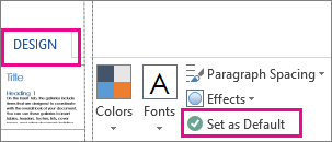
Make my changes the new default theme
After saving your theme, you can set it so it’s used for all new documents.
Excel
Apply your custom theme to a blank workbook and then save it as a template named Book.xltx.
On the Design tab, click Set as Default.
More about themes
A document theme is a unique set of colors, fonts, and effects. Themes are shared across Office programs so that all your Office documents can have the same, uniform look.
You can also change the Office theme. The Office theme is the color scheme for your entire Office program, while document themes are more specific (they show up in individual Word documents or Excel spreadsheets).
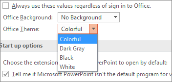
In addition, you can add a pattern to your Office program, by changing the Office Background.
Источник
How to change the default colors that Excel uses for chart series
To change the colors of the current workbook
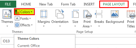
1. On the Page Layout tab, in the Themes group, click Theme Colors:
2. Click Customize Colors. :
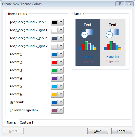
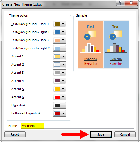
3. In the Create New Theme Colors dialog box, under Theme colors, click the button of the theme color element that you want to change:
4. Under Theme colors, select the colors that you want to use:
In the Create New Theme Colors dialog box, under Sample, you can see the effect of the changes that you make.
5. Repeat steps 3 and 4 for all of the theme color elements that you want to change.
6. In the Name box, type an appropriate name for the new theme colors.
Note: To revert all theme color elements to their original theme colors, you can click Reset before you click Save.
To make changes apply to all new workbooks
If you would like to make these color changes apply to all new workbooks that you create, you need to create a default workbook template.
1. On the Page Layout tab, in the Themes group, click Themes.
2. Click Save Current Theme. :
3. In the File Name box, type an appropriate name for the theme.
Note: A customs document theme is saved in the Document Themes folder and is automatically added to the list of custom themes.
4. On the File tab, choose Save As.
5. In the Save Current Theme dialog box, was selected Office Theme (*.thmx) and chose the Document Themes folder as the location. You can use your own filename instead of the proposed Theme1.thmx.
The location of the Document Themes folder may vary, but it is usually located here:
C:Users AppData Roaming Microsoft Templates Document Themes
Источник
Reader Raja writes in to ask,
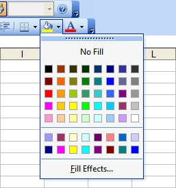
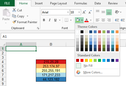
In my spreadsheet, when I wanted to change a cell color, the palette looked like this than the conventional. Its not happening always.
Only a few examples. But when I try to open and close the same file several times, its working fine.Why is it so? Need your help to solve this.
 In my spreadsheet, when I wanted to change a cell color, the palette looked like this than the conventional. Its not happening always.
This happens often in excel 2003 and earlier versions and is annoying when you like to work with certain colors and see them missing from the palette. (if you are wondering, the color management in excel 2007 is much more complicated, we will save it for another day)
Here are few reasons why this might be happening:
- The workbook you have opened has a different palette than the default color scheme of excel 2003. Someone might have changed the colors and now excel is showing you the updated colors.
- You have some excel add-ins that are changing the colors through VBA either when you run them or when you open certain workbooks.
And Here is how you can fix it:
Just go to Menu > Tools > Options > Colors tab, click on “Reset” button. This will reset your palette to excel 2003 default settings.Save the workbook and the colors should now be adjusted as per default scheme.

While there, you can also modify colors if you dont like the default scheme.
More on Excel Colors : How to surpass the 56 color limit in excel 2003 and earlier ?
Share this tip with your colleagues

Get FREE Excel + Power BI Tips
Simple, fun and useful emails, once per week.
Learn & be awesome.
-
16 Comments -
Ask a question or say something… -
Tagged under
colors, excel 2003, excel options, howtos, Learn Excel, microsoft, MS, reader questions, spreadsheets, tips
-
Category:
Excel Howtos, Learn Excel

Welcome to Chandoo.org
Thank you so much for visiting. My aim is to make you awesome in Excel & Power BI. I do this by sharing videos, tips, examples and downloads on this website. There are more than 1,000 pages with all things Excel, Power BI, Dashboards & VBA here. Go ahead and spend few minutes to be AWESOME.
Read my story • FREE Excel tips book


Excel School made me great at work.
5/5

From simple to complex, there is a formula for every occasion. Check out the list now.

Calendars, invoices, trackers and much more. All free, fun and fantastic.

Power Query, Data model, DAX, Filters, Slicers, Conditional formats and beautiful charts. It’s all here.

Still on fence about Power BI? In this getting started guide, learn what is Power BI, how to get it and how to create your first report from scratch.

- Excel for beginners
- Advanced Excel Skills
- Excel Dashboards
- Complete guide to Pivot Tables
- Top 10 Excel Formulas
- Excel Shortcuts
- #Awesome Budget vs. Actual Chart
- 40+ VBA Examples
Related Tips
16 Responses to “Excel Colors Somehow Getting Changed ?”
-
 Mike says:
 I find a couple of annoying things with excel 2003 colours:
1. When I am using cognos or other programmes to pass excel form reports to excel there’s no predicting how the colours translate. Admittedly this may not be excel’s fault.
2. There is something strange about the yellows. I love the pale yellow but hate the bright yellow, yet sometimes it seems to switch to using the bright yellow when you were using the light yellow. I’m wondering if I can customise the bright yellow to a soft yellow to stop it being used?
-
@Mike: you can customize yellows (or just about any color) from the excel options dialog. Modify the color to your favorite RGB and save it as a palette and use it whenever you need. That is a way to avoid some of the ugly colors in excel 2003 default panel. Of course, there will be quite a few manual steps involved in this, usually this is where macros will come handy. Write once and run whenever you need to clean up the charts.
-
Dave says:
This did not work for me…this is extremely annoying as I have a project I’ve been working on for weeks and all of the colors look ridiculous!
-
Chris says:
This did not work for me either. Excel is randomly changing the colour pallet. What gives?!?!
-
@Dave… It can be a macro or setting in some other open workbook that is causing this. Can you close all workbooks, exit excel, open the file once again and reset the palette?
Btw, what version of excel you have?
-
Stephen Spills says:
Oh this is fabulous! I had been literally pulling my hair out about missing my lovely peach color that I use to delineate between expense and capital on my spreadsheet (capital is ALWAYS mint green and peach just seems so right for expense tracking). Anyway, I followed these quick easy steps, 1…2…3… and viola my expense cells turned back to peach after some evil incident caused them all to go drab dead fish grey! FABULOUS!
Kisses and rainbows to all!
Stephen! -
Simon says:
Thanks, this has massively helped with a report I was creating that all of a sudden had the colour scheme thrown right out. @Dave, can confirm the response from Chandoo works. Need to close all spreadsheets down, then re-open the one, use the process originally noted and original preferred colour scheme should return. Thanks again guys!
-
Eric says:
I had this problem too but Chandoo’s solution didn’t help. For those in the same case, give it a try to the true colors add-in from the link before. You’ll be surprised!
-
Lynn says:
Here is how I solved this problem. Close the workbook with the color problem. Close Excel. Open Excel back up. Open a workbook that does not have the color pallette problem.
Now open the workbook with the problem.
TOOLS
OPTIONS
COLOR tab
MODIFY tab
STANDARD tab
There is a Hexagon in the lower right. Click on it and make it black
Now the box with «New» above and «Current» below should be black.
Click «OK»
Click «OK» again to leave the Options and your workbook should be okay.SAVE IT!!
-
Zsombor says:
Thanks Lynn!
Your post was the most helpful, but for me, something slightly different worked.
When you have the non-problem workbook open as well as the problem workbook, go to TOOLS>OPTION>COLOR and choose the working color palette file from the ‘copy colors from’ dropdown list. The files have to be open in the same instance of Excel for this to work, and the other files to appear in the drop down list.
As to how this starts, I run a VBA-report-constructing workbook which sometimes mucks up the palette fo all concurrent Excel files. Very annoying!
Cheers
-
-
Cassie says:
Thank you! This worked perfectly for me. I was going nuts thinking that all my things that were once colored orange which turned brown would just have to stay that way forever. Brown is not a good color for my company spread sheets.
-
Andrea says:
I have a big problem with Excel 2013! I need help, really and I hope someone help me, because it have a big influence in my job.
The problem is: When I create a chart, Excel put series colours automatically, but I change them to other colors I need to be represented. Later, or when I close excel, or when I close the pooled data or when I change to another sheet, series colours return to the predeterminate colours, and it occurs all the time. All my work of changing series colours is going away everytime. And it costs me a lot of time.
So.. If someone please, can help me, would be so greate!
:S-
Stacy says:
Did you ever resolve the issue? It happens to me to too and I hate when I send the report over to my boss and he presents the information in non-company colors! ugh!!
-
-
Andrea says:
Oh! I forget to explain another problem!
The second problem is: When I do the same as before, To change to another sheet or to close Excel or to close pooled data, what I’ve selected to appear on horizontal axis data, became predeterminate again! For example, I putted on horizontal axis 01MAR12 20APR12 14MAY12, … and it changed to 1 2 3 4 ….!!! why???
This changes to the predeterminate configuration occurs in series colours and in horizontal axis data.. and nobody knows why.
Ty very much!
-
Svetlana says:
Unfortunately, the reset did not work. Nothing happened at all.
Leave a Reply
You can highlight data in cells by using Fill Color to add or change the background color or pattern of cells. Here’s how:
-
Select the cells you want to highlight.
Tips:
-
To use a different background color for the whole worksheet, click the Select All button. This will hide the gridlines, but you can improve worksheet readability by displaying cell borders around all cells.
-

-
-
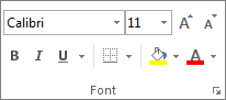
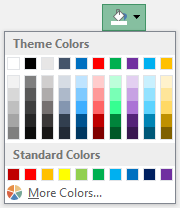
Click Home > the arrow next to Fill Color
, or press Alt+H, H.
-
Under Theme Colors or Standard Colors, pick the color you want.
To use a custom color, click More Colors, and then in the Colors dialog box select the color you want.
Tip: To apply the most recently selected color, you can just click Fill Color
. You’ll also find up to 10 most recently selected custom colors under Recent Colors.

 , or press Alt+H, H.
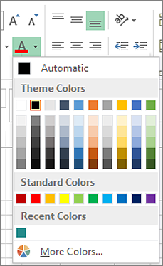
Apply a pattern or fill effects
When you want something more than a just a solid color fill, try applying a pattern or fill effects.
-
Select the cell or range of cells you want to format.
-
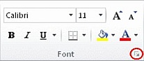
Click Home > Format Cells dialog launcher, or press Ctrl+Shift+F.
-
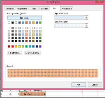
On the Fill tab, under Background Color, pick the color you want.
-
To use a pattern with two colors, pick a color in the Pattern Color box, and then pick a pattern in the Pattern Style box.
To use a pattern with special effects, click Fill Effects, and then pick the options you want.
Tip: In the Sample box, you can preview the background, pattern, and fill effects you selected.
Remove cell colors, patterns, or fill effects
To remove any background colors, patterns, or fill effects from cells, just select the cells. Then click Home > arrow next to Fill Color, and then pick No Fill.
Print cell colors, patterns, or fill effects in color
If print options are set to Black and white or Draft quality — either on purpose, or because the workbook has large or complex worksheets and charts that caused draft mode to be turned on automatically — cells won’t print in color. Here’s how you can fix that:
-
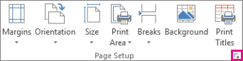
Click Page Layout > Page Setup dialog box launcher.
-
On the Sheet tab, under Print, uncheck the Black and white and Draft quality check boxes.
Note: If you don’t see colors in your worksheet, it may be that you’re working in high contrast mode. If you don’t see colors when you preview before you print, it may be that you don’t have a color printer selected.
If you’d like to highlight text or numbers to make the data more visible, try either changing the font color or add a background color to the cell or range of cells like this:

-
Select the cell or range of cells for which you want to add a fill color.
-
On the Home tab, click Fill Color, and pick the color you want.
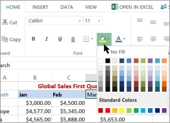
Note: Pattern fill effects for background colors are not available for Excel for the web. If you apply any from Excel on your desktop, it won’t appear in the browser.
Remove fill color
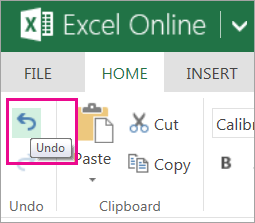
If you decide that you don’t want the fill color immediately after you added it, just click Undo.
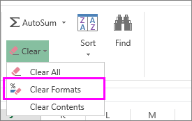
To remove the fill color at a later time, select the cell or cell range you want to change, and click Clear > Clear Formats.
Tuesday, September 3, 2013
Peltier Technical Services, Inc., Copyright © 2023, All rights reserved.
When you know how Excel’s color system works, you can do some great work. We’ll take a brief look backwards at the rudimentary color palette of Classic Excel, then explore the enhanced capabilities of the color system introduced in Office 2007.
The Color Palette (Excel 2003 and Earlier)
You may remember the default color palette of Excel 97 through 2003, shown below. The palette a mishmash of blindingly bright tiles amidst a multitude of dark gloomy colors. I think it was designed by someone who only came out of his dungeon at night.
There were 56 colors in the palette, and you could independently modify any of them. But you could not use any colors beside these 56 in your workbook, except in AutoShapes. Each workbook could have its own palette (but only one palette), and you could assign one workbook’s palette to another workbook. The sixteen tiles in the bottom two rows were not always available for general editing, but were reserved for chart lines (bottom row) and chart fills (second row from the bottom).
What I miss about Excel 2003 is not so much the available colors in the palette, but the fact that you could tear them away from the toolbars and drag them to where you were working. They stayed open until you closed them, which saved hundreds of clicks a day (or hour), and their proximity to your work saved miles and miles of mouse travel.

In fact, Classic Excel contained a variety of formatting tearaway toolbars, and I miss all of them. Here is a screenshot of many of them, in case you’re nostalgic. (Sniff.)
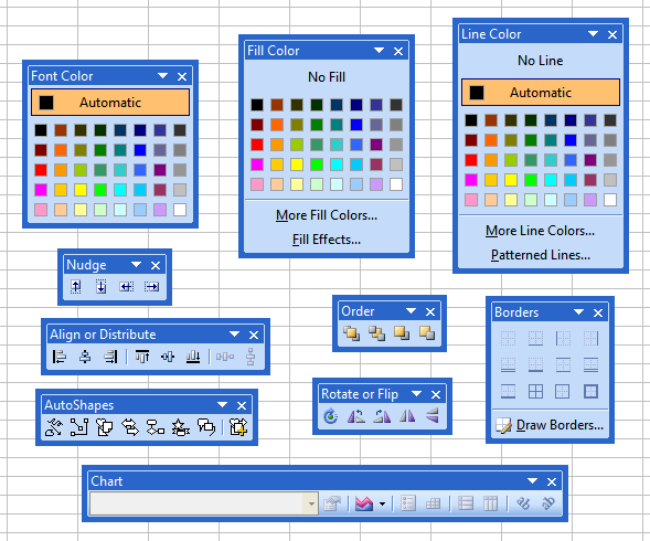
The best thing that Microsoft could do for Excel 2016 would be to reintroduce this kind of old-school functionality, and restore our lost productivity.
The default palette was pretty grim, and the defaults made for some butt-ugly charts. But it was easy enough to tailor your own palette, as I had done with guidance from the color picker at ColorBrewer2.org, thanks to Cynthia A. Brewer, Pennsylvania State University. Below are shown the default palette (left) and one of my custom palettes (right). My bottom three rows were medium, light, and very light shades of 8 colors; I lightened up the grays in the last column, I replaced the dark colors in the top row, and made one of the dull greens in the middle into one with more life.

When a workbook’s color palette is changed, all colors in the workbook are subject to change.
As attached as we were to Excel 2003’s color system, we welcomed the new color system that came with Excel 2007.
The Color Chooser (Excel 2007-2013)
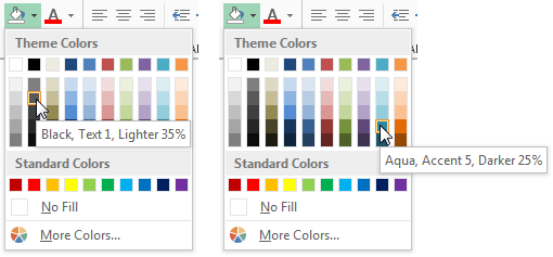
The Classic palette has been replaced with a similar color chooser, which shows all of the colors in the chosen theme. The colors are more organized, where each column of the grid of colors has shades of the same base color. This shows the default Office 2007-2010 theme. The colors are somewhat dull, but they are a major improvement over the Excel 2003 colors, and reportedly these colors are distinguishable by those with the most common color vision deficiencies.
![]()
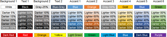
As you mouse over the color chooser, names of the colors pop up. Names like “Black, Text 1, Lighter 35%” and “Aqua, Accent 5, Darker 25%”.
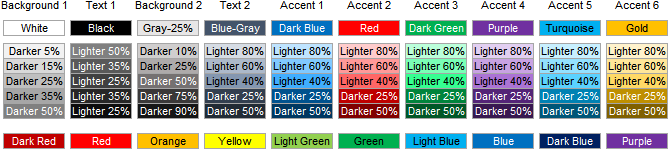
This table shows the names for all color tiles in the default Office 2007-2010 theme. The name consists of the color name in the first row, “Aqua”, then the label from above the table, “Accent 5”, and finally the adjustment of the color, “Darker 25%”.
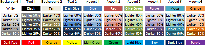
For Text 2 and the Accent colors, the sequence of shades goes Lighter 80%, Lighter 60%, Lighter 40%, Lighter 0%/Darker 0% (the baseline shade), Darker 25%, and Darker 50%. There’s a large jump between the baseline color and the next color at Lighter 40%. I wish they’d decided to use Lightness values of 25%, 50%, and 75% instead of the chosen 40%, 60%, and 80%. I also wish there was a way via the user interface to adjust this percentage, but you need VBA if you want to keep a color associated with the theme.
Theme Colors
We’ve been looking at the default Office 2007-2010 color theme, but there are many more to choose from, which you can access from the Page Layout tab. Office 2013 has a new theme, which is a little livelier than the old 2007-2010 theme, further improving on the Classic Excel colors. There are a slew of other themes too, but it seems most of them are skewed to much towards a particular color to be good for general use.
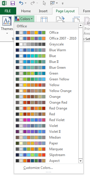
Below are the color choosers for the Office 2007-2010 default theme (left) and the Office 2013 default theme (right). The 2010 theme’s colors are somewhat drab, although a major improvement over the default Excel 2003 palette, and reportedly friendly to those with color vision deficiencies. The Office 2013 colors are brighter, and look very good in charts. I’ve actually grown to like working in Excel 2013, much more than in 2010 and especially in 2007; I suspect the happier colors have contributed to my acceptance of 2013.

Here are the names of the colors in the Office 2013 theme. The color names have changed, but the percentages are all the same. Also, the standard colors are unchanged.
At the bottom of the list of color themes is a button labeled Customize Colors, which leads to this dialog. It is populated below with the Office 2013 colors. There is a preview of how the colors look together, and each color dropdown opens a color picker that lets you access all 16+ million combination of red, green, and blue pixels. then you can name and save your custom theme.

Here I’ve populated the accent colors with pure, fully saturated versions of the Office 2007-2010 theme.
Whoa, that’s pretty bright…
Here are the color names for my custom palette. Notice that Excel tries to guess the names of the colors, or it probably has a lookup table. Turquoise, for example, is somewhat deeper than Aqua.
Notice also the percentages. These are locked in. You can’t change them in the theme color dialog above, you can only change the main colors in the first row.
As with Classic Excel, each workbook has its own theme, which may be shared with other workbooks through the custom theme mechanism. But you could use other colors, including the standard colors from the bottom row, and using the color dialog (More Colors) you could access all the millions of colors available to Windows.
When a workbook’s color theme is changed, all colors that were selected from the theme are subject to change, but any colors defined using More Colors will remain unchanged.
More Colors (Custom or “Recent” Colors)
At the bottom of the color picker is a button labeled More Colors.
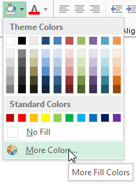
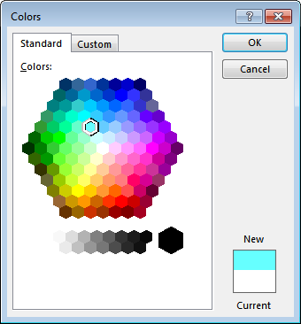
This opens the familiar old Colors dialog used in Classic Excel and a gazillion other applications. The Standard tab shows a hexagonal pattern of colors, with the color of the selected object highlighted in the hex and along the bottom if the color lies on the white-to-gray-to-black axis.
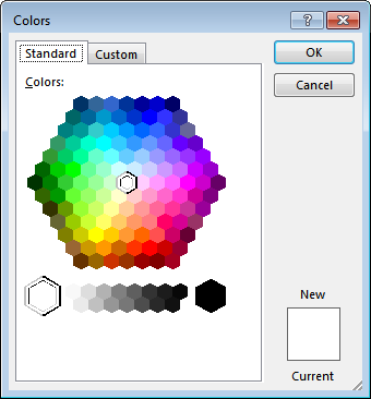
If you select a different color, the New/Current graphic in the bottom corner lets you compare the newly selected color with the original color.
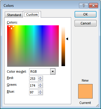
If the hex doesn’t provide just the proper shade, click on the Custom tab. You can change the color by dragging the white crosshairs in the hue-saturation rectangle to the left, or by dragging the black triangle up and down the luminance slider. Or if you know the RGB values you can simply type them into the boxes. The New/Current graphic updates as you adjust the color.

You can also select the HSL color model and enter hue, saturation, and luminance values directly.

When you’ve selected a new color, it appears in a new category of Recent Colors. You can select as many different colors as you need, but only the ten most recently used colors stay in the color chooser.
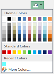
Chart Colors
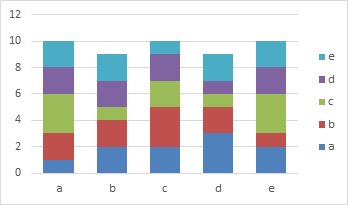
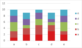
Remember those Excel 2003 charts? Here’s a simple stacked column chart.
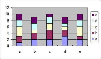
Professor Tufte’s nightmare.
It’s a little better when I use my custom Excel 2003 palette, but there are still too many dark lines everywhere.

If you clean up the dark lines, the Excel 2003 chart doesn’t look too bad.
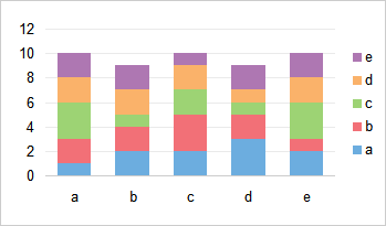
Here’s the chart using the default Office 2007-2010 color theme. Legible but pretty drab except for the aqua bars on top. Much better than the default 2003 chart, though.

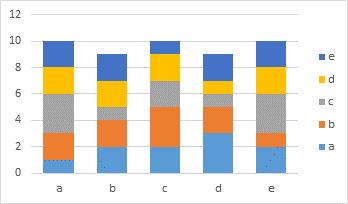
Here is the same chart after changing to the Office 2013 theme. I can’t say that it’s any more legible, but less drab is good.
Here I’ve applied my bright and bold custom theme.
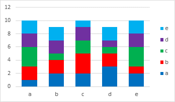
Ouch! It’s a good reminder to use a reputable source for your color scheme. As mentioned earlier, one good source is the color picker at ColorBrewer2.org, thanks to Cynthia A. Brewer, Pennsylvania State University.
Formatting Chart Colors
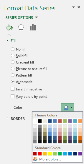
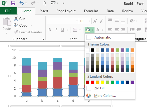
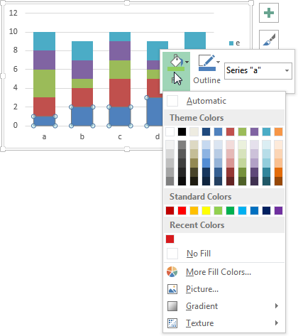
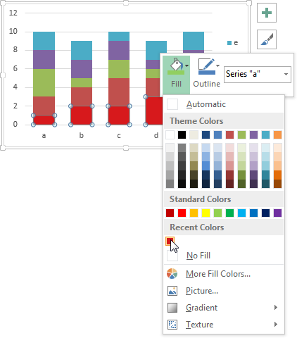
Once you have your chart, there are many ways to format its elements. I’ll illustrate with formatting the fill color of one of the series in the column chart.
One of the most useful shortcuts in Excel is Ctrl+1 (that’s the numeral one). I use it so much I find myself trying to use it in other programs, and it never does anything.
What Ctrl+1 does in Excel is open the formatting dialog or task pane for the selected object. Of course, you could right click on the object and choose the Format [Object Name] button from near the bottom of the pop-up menu, but Ctrl+1 is cooler.
So select the series in the chart and click Ctrl+1 and in Excel 2013 the Format Data Series task pane opens. Its default position is docked to the right edge of the workbook window. I’ve clicked the Fill Color dropdown, and the familiar color chooser pops up.
The taskbar can be undocked by clicking on its top edge and dragging it to where you want to use it. In this way it somewhat resembles the long lost floating tearaway toolbars from Classic Excel. Somewhat.
I’ve floated the task pane over the chart and clicked the Fill Color dropdown to reveal the color chooser.
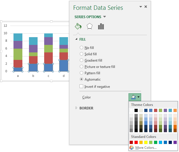
The formatting task pane was introduced in Excel 2013. In Excel 2007 and 2010 there is a formatting dialog, which floats modelessly over the worksheet. When you select the Solid Fill option, the Fill Color dialog appears, and clicking it shows the color chooser.

In Excel 2013 and 2010, but not in 2007, when you right click on a chart element, in addition to the standard pop-up menu, there is a small floating formatting mini-toolbar which has context-relevant formatting buttons (Fill and Outline are displayed below) and a chart element dropdown that identifies the selected element and allows you to select any other element in the chart.
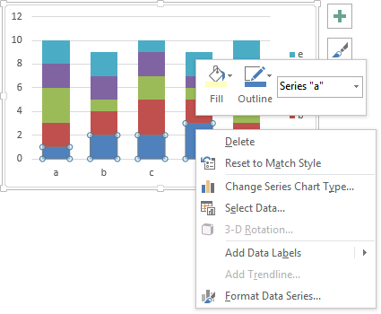
Click on the Fill button, and the color chooser appears.
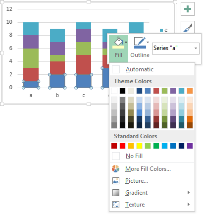
Now for the cool part. When you mouse over a color tile in the chooser, the selected element temporarily takes on the color of that tile, giving you a preview of how the element will look with that color applied. The formatting task pane in Excel 2013 and the formatting dialog in Excel 2007 and 2010 do not give you this preview.
You can also use the controls on the Chart Tools > Format tab to format the chart elements. Select the series and click the Shape Fill button to reveal the color chooser.
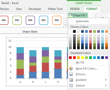
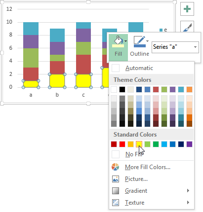
Mouse over a color tile, and as before the selected series is previewed with that fill color. Nice.
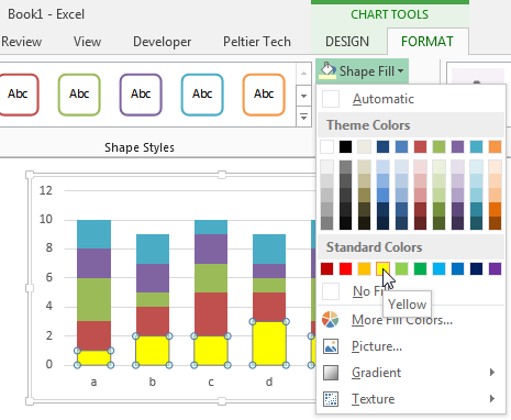
You can even format some elements of the chart using controls on the Home tab. Even though it’s in the Font group of controls, the Fill dialog works on the selected series. Click on the paint can and the color chooser pops up.
Mouse over a color tile, and the series is filled with that color.
That preview feature is pretty cool, a good reason to use anything but the format task pane or dialog for most formatting actions. These protocols work the same for line or border colors, font properties, etc., and the previews are featured when controls on the right-click mini-toolbar or ribbon are used.
Using Copied Custom Colors
Let’s return to our original stacked column chart. We’re going to change the series colors so they range from red-orange at the bottom to blue at the top.
How do you get the colors into the chart? Well, you can define other colors by entering RGB values, but if you have more than a few, you’ll get pretty bored. I have a method that’s much more fun.
I have several worksheets on which I have stored various color sequences, based on the work at ColorBrewer2.org, thanks to Cynthia A. Brewer, Pennsylvania State University. If that name sounds familiar, it’s because I keep mentioning it, and you should visit the site and find some decent color schemes.
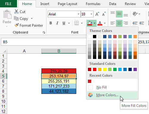
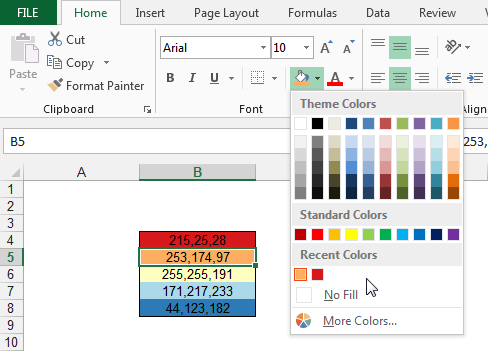
Here is a small view of one of my color worksheets. The columns are color schemes (red-blue, orange-purple, etc.), the rows are groups of three colors, five colors, seven colors, etc. each cell is shaded with the particular color, and the RGB values are shown in the cell for reference.
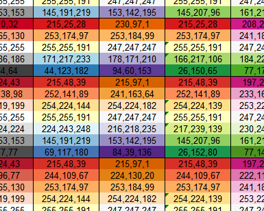
I usually start by copying the block of cells with the colors I want, and paste them somewhere in the workbook.

The color chooser in a new workbook shows the default color theme and standard colors, and no recently used colors. Here’s an easy way to get the colors from the copied range into the Recent Colors section of the chooser. Remember there’s a limit of ten recent colors.
Select one of the colored cells. Click on the Fill dropdown, and then click More Colors at the bottom of the color chooser.
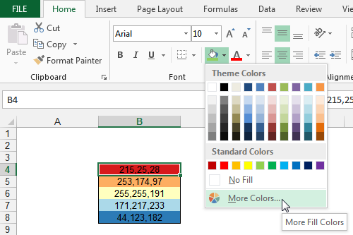
The Colors dialog pops up. When a color-theme-formatted object is selected, the current color in the Colors dialog is black and the standard tab is active. However, when an object formatted with a custom color is selected, its RGB values are plotted on the Custom tab, and the Current/New graphic shows this color.
Don’t make any changes in this dialog, just click OK to close it. Now when we check the color chooser, the color that we saw in the Colors dialog appears in the Recent Colors list.

That was easy, we didn’t have to type any numbers or anything.
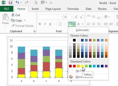
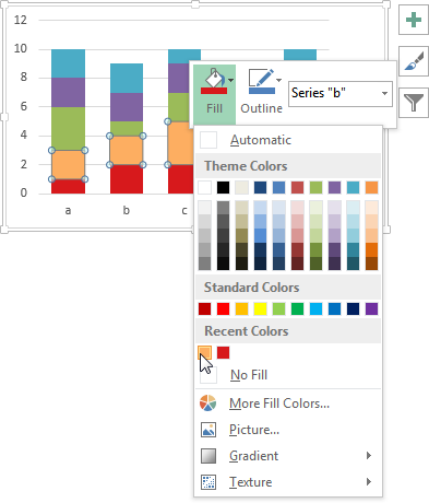
Now we can select the series we want to format and click the Fill dropdown to reveal the color chooser. Yes, the newly added custom color is still there.
Mouse over the new color, and behold the series previewed with that color.
Release the mouse and the chart series has been filled with the new custom color.
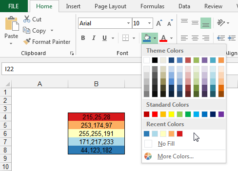
Select the next colored cell, click the Fill dropdown, and click More Colors.
The new cell’s fill color is plotted in the Colors dialog.
Click OK to insert this color into Recent Colors.
Return to the chart, right click the next series click the Fill button, mouse over the new color in the chooser, and the color is previewed in the series.
Here’s the chart, 2/5 of the way done.
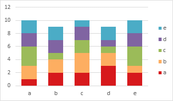
Lather, rinse, repeat until all of the colors have been added to Recent Colors.
Here is the chart with our desired color scheme applied.

The workbook will remember these colors when it is closed and reopened. The recent color tiles will rearrange themselves, with the most recently used color furthest to the left. This makes the most recent color easy to find when you’re applying the color to many objects.

Further Investigation
Office 2007 Colors
This article has covered most of the user interface part of Excel’s colors. With some VBA and the patience to flush out details of the object model, you can further expand Excel’s capabilities. Of course, the object model that came out with Office 2007 was somewhat half-baked, and there were problems with some combinations of color and percentage brightness or darkness not being obtainable. Some new VBA elements were introduced in 2010 that fixed a few problems and seemed to have added some of their own.
For further coverage of Office 2007’s color mechanisms, check out Tony Jollans’ article, Colours in Word 2007. Tony has spend lots of time figuring out and documenting Office 2007’s colors in excruciating detail.
Echo Swinford shows how to hack the XML code of the theme to add your own Custom Colors to the color chooser in PowerPoint 2007 Custom Colors. These are different from Recent Colors and appear in a Custom Colors section above the Standard Colors section.
Mr. Spreadsheet himself, John Walkenbach, covered Office 2007 colors in Excel 2007 VBA Challenge, More On Office 2007 Colors, and Exploring Theme Colors, in which he describes some of the glitches he’s encountered.
Choosing Colors
I’ve mentioned several times that good colors can be found at ColorBrewer2.org, thanks to Cynthia A. Brewer, Pennsylvania State University. There are innumerable color scheme designers on the web, but I prefer ColorBrewer’s complete schemes.
Perceptual Edge hosts an article by Maureen Stone, Choosing Colors for Data Visualization, as well as Stephen few’s articles Practical Rules for Using Color in Charts and Uses and Misuses of Color.
Juice Analytics has some advice about color use in Color Has Meaning and other pages linked from that one.
NASA has an extensive library of pages about Using Color in Information Display Graphics.
UXmatters has a series of articles about Color Theory for Digital Displays: A Quick Reference: Part I, Part II, and Part III.
To check your colored images for color vision deficient viewers, visit Vischeck.
If you search for “Excel colour codes” you will find sites that list Excel’s 56 “official” colours. You will not find any of numbers you list in the official list.
The Red, Green and Blue values for the numbers you list are:
             Red   Green   Blue
10855845     165     165    165
10921638     166     166    166
 9868950     150     150    150  Grey 40%

14922893     141     180    227
14857357     141     180    226
16764057     153     204    255  Pale blue

14211288     216     216    216
14277081     217     217    217
12632256     192     192    192  Grey 25%
In each sub-table, the first two lines show your colour numbers. Although the combined numbers like very different, you will notice the separate values are almost identical so the two alternative colours would look the same on the screen. The third line shows the nearest official Excel colour and its name.
The question for you to investigate is: where have these non-standard colour numbers come from? Are these colours being set by a program or has the palette been very subtly changed by a user? I find it difficult to believe Microsoft released Excel 2007, 2010 and 2013 to you in this state.
New section
I have been playing with Excel colours and I am convinced your problem is related to the palette and the use of non-standard colours.
I do not have your range of versions so experimented with 2003 and 2007.
With 2003 there is a palette of 56 colours and a colour index with a value of 1 to 56. I believe that Excel stores the colour index against a cell because:
- If with VBA you set a cell to an off-palette colour, Excel immediately changes it to an on-palette colour.
- If you change a colour on the palette, every use of that colour within the workbook immediately changes.
That is, with 2003 you can have any 56 colours but only 56 different colours.
Under 2003, I created a new workbook. On the palette, I switched Red and Blue and I replaced Indigo, RGB(51, 51, 163), by RGB(167, 167, 167). This is not a standard Excel colour but, if it was, it would be named something like Grey 30. I coloured a few cells using these colours.
I opened this workbook with 2007 and saved it as an xlsm file. The colours on the worksheet appeared unchanged. I selected a new cell and defined a custom colour of RGB(167, 167, 167). Visually the new cell was identical (to my eyes) to those coloured with the RGB(167, 167, 167) imported from 2003. I then examined these cells via the palette and VBA:
Colour I    Appearance   Number according      Number according
had set     on screen    to palette            to VBA
255,0,0       Red        0,0,255 Blue          255,0,0
0,0,255       Blue       255,0,0 Red           0,0,255
167,167,167   Grey 30    51,51,153 Indigo      167,167,167      Imported from 2003
167,167,167   Grey 30    167,167,167 Grey 30   167,167,167      Created with 2007
The implication from the last line is that 2007 can handle custom colours correctly if defined within 2007 but gets hopelessly confused with imported custom colours.
My understanding is that 2007 to 2010 to 2013 involved incremental improvements but 2003 to 2007 was a total rewrite. I would guess a bug in 2007 was fixed in 2010.
I believe the problem is the use of non-standard colours. 2007 may have a larger standard palette but RGB(167, 167, 167) is not on it. I do not have 2010 or 2013 but suspect I would get different results if I tried this experiment with either of them.
I believe you must re-colour all cells that use these custom colours with standard colours. You report two custom shades of grey and a custom variation of pale blue. Surely 2007, 2010 and 2013 offer enough standard shades and colours?
Themes available in Excel are used in formatting the entire document or workbook. We can use the themes provided by Excel or customize them according to our choice. Themes are available in Excel in the “Page Layout” tab with the name of the “Themes” option. In addition, there are different options for colors and effects fonts.
Table of contents
- Themes For Excel
- Where are the Themes Stored in Excel?
- Examples
- Example #1 – Change Default Theme
- Example #2 – Change the Row Header & Column Header View
- Example #3 – Create Your Own Theme Under Custom Theme
- Things to Remember
- Recommended Articles
Where are the Themes Stored in Excel?
The first question is, where are these themes hidden in Excel? The truth is that it is not hidden in Excel. Rather, it is visible just before us, but we have not recognized it for long.
Themes are available under “Page Layout” in Excel. So, for example, under “Themes,” we have themes, colors, fonts, and effects.
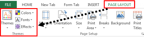
Excel 2013 has as many as 31 built-in themes, 23 colors, and 15 different built-in effects.
Examples
Example #1 – Change Default Theme
Now, we will see the practical example of themes.
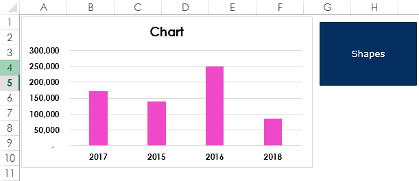
- But, first, we have created a basic default chart of sales for many years and one of the shapes.

- These are the themes of the default theme of the office. To change the theme of these two: charts and shapes, go to “Page Layout.” The above available themes will preview the result before clicking on it.

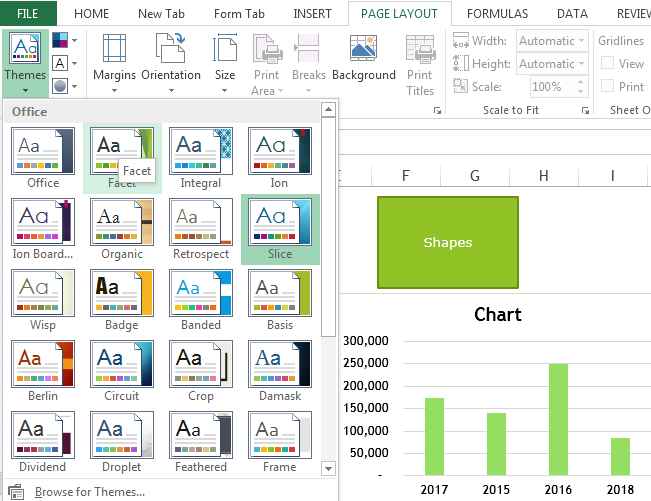
- In the above image, we selected the theme type “Facet.” Like this, we can choose any of the above themes, look at the preview, and finalize the theme.


Example #2 – Change the Row Header & Column Header View
You must be familiar with the default row headerExcel Row Header is the grey column on the left side of column 1 in the worksheet that contains the numbers (1, 2, 3, etc.). To hide or reveal row and column headers, press ALT + W + V + H.read more and column header, which Microsoft gives, like the one below.
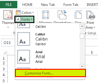
Step 1: Go to “Page Layout” and select “Fonts.”.
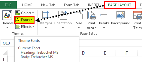
Step 2: Click on the dropdown and select “Customize Fonts.”
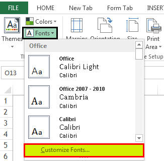
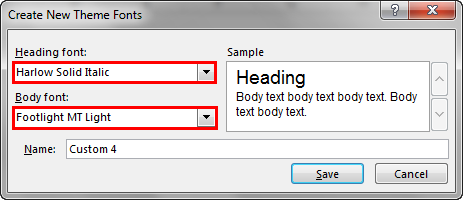
Step 3: Now, you will see below the new dialog box.

Step 4: Change the “Heading font” to “Harlow Solid Italic and the “Body font” to “Footlight MT Light.” Now, on the right-hand side, you can see the preview.
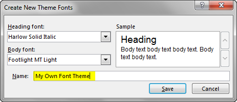
Step 5: You can name this font theme.
Now, look how row and column headers fonts have changed.
It is slightly different from the default theme.
Example #3 – Create Your Own Theme Under Custom Theme
If you are not satisfied with the available wide variety of themes from Microsoft, you can create your theme and apply it to make a difference.
Usually, the theme is the makeup of three elements: colors, fonts, and effects. To design your theme, follow the below steps.
Step 1: Go to “Page Layout” and select “Colors.”
Step 2: Click on the colors drop-down list in excelA drop-down list in excel is a pre-defined list of inputs that allows users to select an option.read more and select “Customize Colors.”

Step 3: Apply the colors below (you can give your colors), name your theme, and click on “Save.”
Step 4: Now, click on “Fonts” and select “Customize Fonts.”
Step 5: Select the fonts as per your wish.
Note: We cannot change the font size. It will be, by default, 11 sizes.
Step 6: Click on “Effects” and select any one of the existing effects. We cannot customize this. We have chosen one of the current effects.
Now, we have created all theme options.
Step 7: Click on the “Theme” dropdown and select “Save Current Theme.”
Step 8: Now, we will see a different save window. Please give them a name and select the “Save type” as “.thmx.“
Now, we have created our theme. When the Excel workbook opens, we can see this theme under Page Layout > Theme > Custom.
Things to Remember
- It will not be available if we share the file with a custom theme with the colleague theme. But theme color and font styles will be applicable.
- The theme applies to Excel charts, tables, shapes, slicers, and pivot tablesA Pivot Table is an Excel tool that allows you to extract data in a preferred format (dashboard/reports) from large data sets contained within a worksheet. It can summarize, sort, group, and reorganize data, as well as execute other complex calculations on it.read more.
- We must use very light colors in the custom themes.
Recommended Articles
This article is a guide to Themes in Excel. Here, we discuss applying different themes in Excel with examples and downloadable Excel templates. You may learn more about Excel from the following articles: –
- Excel Chart Animation
- Excel Marimekko Chart (Mekko)
- Organization Chart in Excel
- Flow Chart in Excel
- Percentage Change Formula in Excel
My apologies for reopening this post. I have done some troubleshooting with this, and my findings are as follows.
Let’s say that we are using the «Paste Special — All using source theme» option, only your data and formatting from the original worksheet would be retained, floating objects would not be copied over. This option will only work when there are no floating objects (charts, diagrams, shapes) in that worksheet. VBA:
Cells.Copy
Workbooks.Add
Selection.PasteSpecial Paste:=xlPasteAllUsingSourceTheme, Operation:=xlNone _
    , SkipBlanks:=False, Transpose:=False
To have all contents pertaining to a sheet (including floating objects) one would have to move/copy the sheet to the new/destination workbook. Upon doing this, all colours would change to a different theme, including the colours of charts. This is the case even when colour pallets of both workbooks are the same.
I have attached a file for you to play with. Try copying/moving the sheet to a new workbook and see what happens, this file originates from an Office 2010 platform. I am using Office 365 on Win8, and these standard colours change to different shades of yellow and grey.
This problem is not present when you are using workbooks created from scratch in Office 365, but on files created with previous versions of office, the issue is unresolved when used a later version of Office.
THE SOLUTION: Page Layout —> Colours —> Office 2007-2010
And in VBA:
ActiveWorkbook.Theme.ThemeColorScheme.Load ( _
    "C:Program FilesMicrosoft Office 15RootDocument Themes 15Theme ColorsOffice 2007 - 2010.xml" _
    )