
Содержание
- Apply color to alternate rows or columns
- Use conditional formatting to apply banded rows or columns
- How to fill color in excel cell using formula
- How to color a cell in Excel using a formula?
- 2 Answers 2
- How to Count Colored Cells in Excel – A Step by Step Tutorial + Video
- How to Count Colored Cells in Excel
- #1 Count Colored Cells Using Filter and SUBTOTAL
- #2 Count Colored Cells Using GET.CELL Function
- Creating a Named Range
- Getting the Color Code for Each Cell
- Count Colored Cells using the Color Code
- #3 Count Colored Using VBA (by Creating a Custom Function)
Apply color to alternate rows or columns
Adding a color to alternate rows or columns (often called color banding) can make the data in your worksheet easier to scan. To format alternate rows or columns, you can quickly apply a preset table format. By using this method, alternate row or column shading is automatically applied when you add rows and columns.
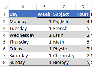
Select the range of cells that you want to format.
Click Home > Format as Table.
Pick a table style that has alternate row shading.
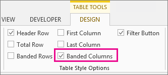
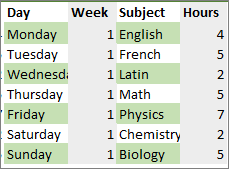
To change the shading from rows to columns, select the table, click Design, and then uncheck the Banded Rows box and check the Banded Columns box.
Tip: If you want to keep a banded table style without the table functionality, you can convert the table to a data range. Color banding won’t automatically continue as you add more rows or columns but you can copy alternate color formats to new rows by using Format Painter.
Use conditional formatting to apply banded rows or columns
You can also use a conditional formatting rule to apply different formatting to specific rows or columns.
On the worksheet, do one of the following:
To apply the shading to a specific range of cells, select the cells you want to format.
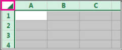
To apply the shading to the whole worksheet, click the Select All button.
Click Home > Conditional Formatting > New Rule.
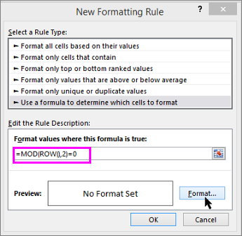
In the Select a Rule Type box, click Use a formula to determine which cells to format.
To apply color to alternate rows, in the Format values where this formula is true box, type the formula =MOD(ROW(),2)=0.
To apply color to alternate columns, type this formula: =MOD(COLUMN(),2)=0.
These formulas determine whether a row or column is even or odd numbered, and then applies the color accordingly.
In the Format Cells box, click Fill.
Pick a color and click OK.
You can preview your choice under Sample and click OK or pick another color.
To edit the conditional formatting rule, click one of the cells that has the rule applied, click Home > Conditional Formatting > Manage Rules > Edit Rule, and then make your changes.
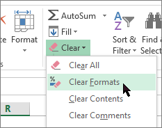
To clear conditional formatting from cells, select them, click Home > Clear, and pick Clear Formats.
To copy conditional formatting to other cells, click one of the cells that has the rule applied, click Home > Format Painter  , and then click the cells you want to format.
Источник
How to fill color in excel cell using formula
A free Office suite fully compatible with Microsoft Office
A free Office suite fully compatible with Microsoft Office
How to fill color in excel cell using formula? You can do this by conditional formatting option. When you use colors in your excel worksheets you can instantly visualize the difference or comparison in value. Additionally, specification of important information gets easy. In order to specify the condition, you can use IF statement and then use conditional formatting to highlight the conditions.
If you are wondering how to fill color in excel cell using formula, here is your guide to it. So, read entire article.
Note: There is only one way to access conditional formatting as below
Use colors under certain conditions
1. Open the document having some data. Here is an example of test grades of students in terms of percentage. In this data many students passed while few failed. If we need to find fail students without wasting time, use conditional formatting.
2. Use the IF statement before applying colors. To do this, click on C3.
3. Now type equals sign and if in this cell. Then press Enter, the IF statement is activated
4. Now go to cell B3, click it and type st part of condition telling if the cell value is less than 40.
5. Now type comma, and then write Fail in inverted commas like this “Fail”
6. Again type comma, and then write Pass in inverted commas. This is the full condition which means that if the value is less than 40, type fail, otherwise pass.
7. When you press Enter key. The Pass word is shown because the student scored more than 40% grades.
8.In order to apply this function to all cells till end, click on the cell C3 again then click the right corner of the cell, drag vertically till B28.
9. Now to apply conditional formatting, click again on cell C3 and go to Conditional Formatting under Home tab. A drop down box appears.
10. Put your mouse at Highlight Cell Rules, a drop down box appears.
11. Click “Text That Contains” option in drop down menu.
12. A dialogue box opens. Now click the arrow at the right of blank field.
13. Now click C3 and press Enter. Notice the value is specified.
14. Now click on the down arrow. A drop box appears to select colors.
15. Click Light Red Fill for this example.
16. Click Ok. The text in cell C3 is filled with light red color.
17. Click on C3 cell, hover mouse at bottom right corner, click and drag. All the text containing word Pass get highlighted.
18. Now to find which student failed, repeat the whole procedure but type Fail in “Text That Contains” dialogue box and select “Green Fill With Dark Green Text” as the color.
19. Press Enter. Nothing happens to C3 as the cell has word Pass.
20. when you click and drag cursor from C3 to C28. All the cells having Fail written get highlighted in different color.
So this is whole process of how to fill color in excel cell using formula. Need to edit Word/Excel/PPT file free of charge? download WPS Office edit files like without any cost. Download now! to get enjoyable working experience.
Источник
How to color a cell in Excel using a formula?
I want to do something like:
I want a formula not a wizard.

2 Answers 2
Instead of using a formula, you should go with conditional formatting. Select the appropriate column and go to Home -> Conditional formatting -> Highlight Cells Rules. Afterwards you can define the criteria, and which color the cell should become.
EDIT:
As far as I am aware of, changing the color of a cell is impossible using a formula. Should someone know how to do it, please post! In the meanwhile, this is a small routine on how to change the color to green using VBA.
Note: This formula should take around 3
6 seconds per 100k rows, which could be rather slow, depending on the application. After running a small test I found the following runtimes:
It seems using Cells(i, 1).Interior.ColorIndex ups the time with a whopping 34s/100k records! If someone knows a better way, feel free to enlighten us!
You can use a formula in conjunction with an Event Macro. Pick a cell, say B2 and enter the formula:
Then format B2 Custom ;;;
This will hide the displayed text.
Then place the following event macro in the worksheet code area:
The macro will run every time the worksheet is re-calculated. It will exame the text in B2 (even though the text is not visible) and adjust the backgound color accordingly.
Because it is worksheet code, it is very easy to install and automatic to use:
- right-click the tab name near the bottom of the Excel window
- select View Code — this brings up a VBE window
- paste the stuff in and close the VBE window
If you have any concerns, first try it on a trial worksheet.
If you save the workbook, the macro will be saved with it. If you are using a version of Excel later then 2003, you must save the file as .xlsm rather than .xlsx
To remove the macro:
- bring up the VBE windows as above
- clear the code out
- close the VBE window
To learn more about macros in general, see:
To learn more about Event Macros (worksheet code), see:
Macros must be enabled for this to work!
Источник
How to Count Colored Cells in Excel – A Step by Step Tutorial + Video
Watch Video – How to Count Colored Cells in Excel
Wouldn’t it be great if there was a function that could count colored cells in Excel?
Sadly, there isn’t any inbuilt function to do this.
It can easily be done.
This Tutorial Covers:
How to Count Colored Cells in Excel
In this tutorial, I will show you three ways to count colored cells in Excel (with and without VBA):
- Using Filter and SUBTOTAL function
- Using GET.CELL function
- Using a Custom Function created using VBA
#1 Count Colored Cells Using Filter and SUBTOTAL
To count colored cells in Excel, you need to use the following two steps:
- Filter colored cells
- Use the SUBTOTAL function to count colored cells that are visible (after filtering).
Suppose you have a dataset as shown below:

There are two background colors used in this data set (green and orange).
Here are the steps count colored cells in Excel:
- In any cell below the data set, use the following formula: =SUBTOTAL(102,E1:E20)

- Select the headers.
- Go to Data –> Sort and Filter –> Filter. This will apply a filter to all the headers.
- Click on any of the filter drop-downs.
- Go to ‘Filter by Color’ and select the color. In the above dataset, since there are two colors used for highlighting the cells, the filter shows two colors to filter these cells.


As soon as you filter the cells, you will notice that the value in the SUBTOTAL function changes and returns only the number of cells that are visible after filtering.
How does this work?
The SUBTOTAL function uses 102 as the first argument, which is used to count visible cells (hidden rows are not counted) in the specified range.
If the data if not filtered it returns 19, but if it is filtered, then it only returns the count of the visible cells.
Try it Yourself.. Download the Example File 
#2 Count Colored Cells Using GET.CELL Function
GET.CELL is a Macro4 function that has been kept due to compatibility reasons.
It does not work if used as regular functions in the worksheet.
Here are the three steps to use GET.CELL to count colored cells in Excel:
- Create a Named Range using GET.CELL function
- Use the Named Range to get color code in a column
- Using the Color Number to Count the number of Colored Cells (by color)
Let’s deep dive and see what to do in each of the three mentioned steps.
Creating a Named Range
Getting the Color Code for Each Cell
In the cell adjacent to the data, use the formula =GetColor
This formula would return 0 if there is NO background color in a cell and would return a specific number if there is a background color.
This number is specific to a color, so all the cells with the same background color get the same number.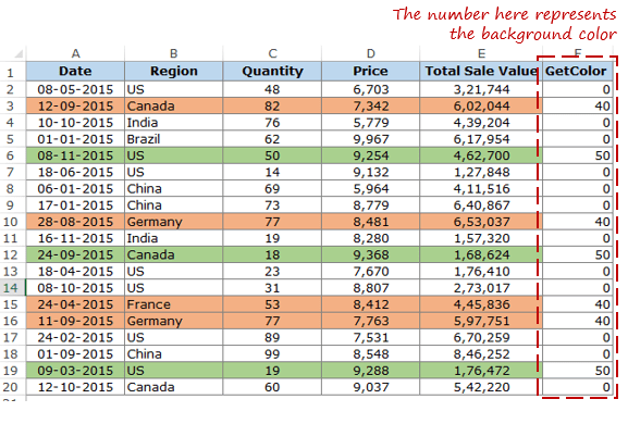
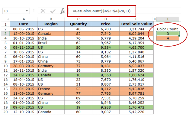
Count Colored Cells using the Color Code
If you follow the above process, you would have a column with numbers corresponding to the background color in it.
To get the count of a specific color:
- Somewhere below the dataset, give the same background color to a cell that you want to count. Make sure you are doing this in the same column that you used in creating the named range. For example, I used Column A, and hence I will use the cells in column ‘A’ only.
- In the adjacent cell, use the following formula:
This formula will give you the count of all the cells with the specified background color.
How Does It Work?
The COUNTIF function uses the named range (GetColor) as the criteria. The named range in the formula refers to the adjacent cell on the left (in column A) and returns the color code for that cell. Hence, this color code number is the criteria.
The COUNTIF function uses the range ($F$2:$F$18) which holds the color code numbers of all the cells and returns the count based on the criteria number.
Try it Yourself.. Download the Example File
#3 Count Colored Using VBA (by Creating a Custom Function)
In the above two methods, you learned how to count colored cells without using VBA.
But, if you are fine with using VBA, this is the easiest of the three methods.
Using VBA, we would create a custom function, that would work like a COUNTIF function and return the count of cells with the specific background color.
Here is the code:
To create this custom function:
To use this function, simply use it as any regular excel function.
Syntax: =GetColorCount(CountRange, CountColor)
- CountRange: the range in which you want to count the cells with the specified background color.
- CountColor: the color for which you want to count the cells.
To use this formula, use the same background color (that you want to count) in a cell and use the formula. CountColor argument would be the same cell where you are entering the formula (as shown below):
Note: Since there is a code in the workbook, save it with a .xls or .xlsm extension.
Try it Yourself.. Download the Example File
Do you know any other way to count colored cells in Excel?
If yes, do share it with me by leaving a comment.
You May Also Like the Following Excel Tutorials:
Источник
You can use a formula in conjunction with an Event Macro. Pick a cell, say B2 and enter the formula:
=IF(A1>10,"black","green")
Then format B2 Custom ;;;
This will hide the displayed text.
Then place the following event macro in the worksheet code area:
Private Sub Worksheet_Calculate()
Application.EnableEvents = False
    With Range("B2")
        If .Value = "green" Then
            .Interior.Color = RGB(0, 255, 0)
        Else
            .Interior.Color = RGB(0, 0, 0)
        End If
    End With
Application.EnableEvents = True
End Sub
The macro will run every time the worksheet is re-calculated. It will exame the text in B2 (even though the text is not visible) and adjust the backgound color accordingly.
Because it is worksheet code, it is very easy to install and automatic to use:
- right-click the tab name near the bottom of the Excel window
- select View Code — this brings up a VBE window
- paste the stuff in and close the VBE window
If you have any concerns, first try it on a trial worksheet.
If you save the workbook, the macro will be saved with it.
If you are using a version of Excel later then 2003, you must save
the file as .xlsm rather than .xlsx
To remove the macro:
- bring up the VBE windows as above
- clear the code out
- close the VBE window
To learn more about macros in general, see:
http://www.mvps.org/dmcritchie/excel/getstarted.htm
and
http://msdn.microsoft.com/en-us/library/ee814735(v=office.14).aspx
To learn more about Event Macros (worksheet code), see:
http://www.mvps.org/dmcritchie/excel/event.htm
Macros must be enabled for this to work!
Adding a color to alternate rows or columns (often called color banding) can make the data in your worksheet easier to scan. To format alternate rows or columns, you can quickly apply a preset table format. By using this method, alternate row or column shading is automatically applied when you add rows and columns.
Here’s how:
-
Select the range of cells that you want to format.
-
Click Home > Format as Table.
-
Pick a table style that has alternate row shading.
-
To change the shading from rows to columns, select the table, click Design, and then uncheck the Banded Rows box and check the Banded Columns box.
Tip: If you want to keep a banded table style without the table functionality, you can convert the table to a data range. Color banding won’t automatically continue as you add more rows or columns but you can copy alternate color formats to new rows by using Format Painter.
Use conditional formatting to apply banded rows or columns
You can also use a conditional formatting rule to apply different formatting to specific rows or columns.
Here’s how:
-
On the worksheet, do one of the following:
-
To apply the shading to a specific range of cells, select the cells you want to format.
-
To apply the shading to the whole worksheet, click the Select All button.
-
-
Click Home > Conditional Formatting > New Rule.
-
In the Select a Rule Type box, click Use a formula to determine which cells to format.
-
To apply color to alternate rows, in the Format values where this formula is true box, type the formula =MOD(ROW(),2)=0.
To apply color to alternate columns, type this formula: =MOD(COLUMN(),2)=0.
These formulas determine whether a row or column is even or odd numbered, and then applies the color accordingly.
-
Click Format.
-
In the Format Cells box, click Fill.
-
Pick a color and click OK.
-
You can preview your choice under Sample and click OK or pick another color.
Tips:
-
To edit the conditional formatting rule, click one of the cells that has the rule applied, click Home > Conditional Formatting > Manage Rules > Edit Rule, and then make your changes.
-
To clear conditional formatting from cells, select them, click Home > Clear, and pick Clear Formats.
-
To copy conditional formatting to other cells, click one of the cells that has the rule applied, click Home > Format Painter
, and then click the cells you want to format.
-
Need more help?
Want more options?
Explore subscription benefits, browse training courses, learn how to secure your device, and more.
Communities help you ask and answer questions, give feedback, and hear from experts with rich knowledge.
How to Sum by Color in Excel? (2 Useful Methods)
The top two methods to Sum by Colors in Excel are as follows –
- Usage of SUBTOTAL formula in excelThe SUBTOTAL excel function performs different arithmetic operations like average, product, sum, standard deviation, variance etc., on a defined range.read more and filter by color function.
- Applying GET.CELL formula by defining the name in the formula tab and applying the SUMIF formula in excelThe SUMIF Excel function calculates the sum of a range of cells based on given criteria. The criteria can include dates, numbers, and text. For example, the formula “=SUMIF(B1:B5, “<=12”)” adds the values in the cell range B1:B5, which are less than or equal to 12.
read more to summarize the values by color codes.
Let us discuss each of them in detail –
Table of contents
- How to Sum by Color in Excel? (2 Useful Methods)
- #1 – Sum by Color using Subtotal Function
- #2 – Sum by Color using Get.Cell Function
- Things to Remember
- Recommended Articles
You can download this Sum by Color Excel Template here – Sum by Color Excel Template
#1 – Sum by Color using SUBTOTAL Function
To understand the approach for calculating the sum of values by background colors, let us consider the below data table, which provides details of amounts in US$ by region and month.

Lets start.
- Suppose we would like to highlight those cells which are negative in values for indication purpose, this can be achieved by either applying conditional formatting or manually highlighting the cells, as shown below.

- To achieve the sum of cells that are colored in excel, enter the formula for SUBTOTAL below the data table. The syntax for the SUBTOTAL formula is shown below.

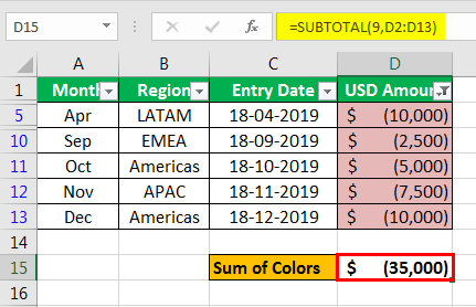
The formula that is entered to calculate the summation is=SUBTOTAL(9,D2:D13)
Here, the number 9 in the function_num argument refers to sum functionality, and the reference argument is given as the range of cells to be computed. Below is the screenshot for the same.

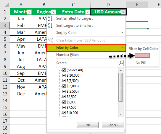
- As the above screenshot shows, a “USD Amount” summation has been calculated to compute the amounts highlighted in a light red background. Next, apply the filter to the data table by going to the “Data” tab and selecting a filter.

- Select filter by color and choose the light red cell color under “Filter by Color.” Below is the screenshot to better describe the filter.

- Once the excel filter has been applied, it will filter the data table for only light red background cells. The subtotal formula used at the bottom of the data table would display the summation of the colored cells, which are filtered as shown below.

As shown in the above screenshot, the computation of the colored cell is achieved in cell E17, subtotal formula.


#2 – Sum by Color using Get.Cell Function
The second approach is explained to arrive at the sum of the color cells in excel, as discussed in the below example. Consider the data tableA data table in excel is a type of what-if analysis tool that allows you to compare variables and see how they impact the result and overall data. It can be found under the data tab in the what-if analysis section.read more to understand the methodology better.

- Step 1: Now, let us highlight the list of cells in the “USD Amount” column, which we are willing to arrive at the desired sum of colored cells, as shown below..

- Step 2: As we can see in the above screenshot, unlike in the first example here, we have multiple colors. Thereby we will be using the formula =GET.CELL by defining it within the name boxIn Excel, the name box is located on the left side of the window and is used to give a name to a table or a cell. The name is usually the row character followed by the column number, such as cell A1.read more and not directly using it in excel.
- Step 3: Now, once the dialog box for the “Define Name” pops up, enter the name and the formula forgetting. CELL in “Refer to,” as shown in the below screenshot.
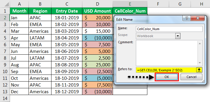
As seen in the above screenshot, the name entered for the function is “CellColor_Num,” and the formula =GET.CELL(38,’Example 2!$D2) is to be entered in ‘Refers to.’ Within the formula, the numeric 38 refers to the cell code information, and the second argument is the cell number D2 refers to the reference cell. Now, click “OK.”
- Step 4: Now, enter the function name “CellColor” in the cell beside the color-coded cell, which was defined in the dialog box, as explained in step 3.

As seen in the above screenshot, the function “CellColor” is entered, which returns the color code for the background cell color.
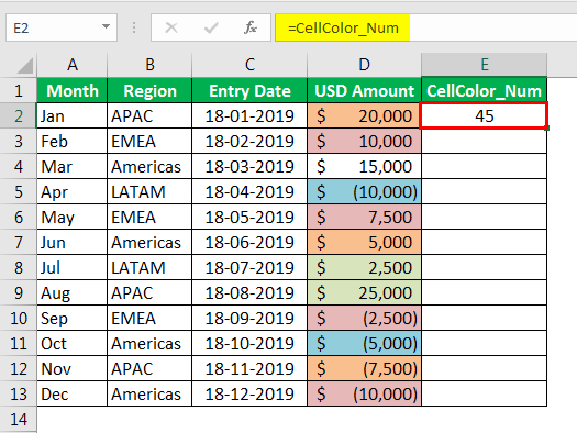
Similarly, the formula is dragged for the entire column.

- Step 5: Now, to arrive at the sum of the values by colors in excel, we will be entering the SUMIF formula. The syntax for the SUMIF formula is as follows:-

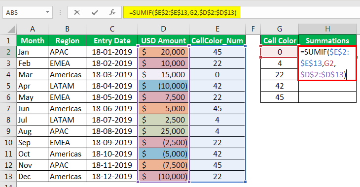
As can be seen from the above screenshot, the following arguments are entered into the SUMIF formula:-
- The range argument is entered for cell range E2: E13.
- The criteria are entered as G2, whose summarized values are needed to be retrieved.
- The range of cells is entered to be D2: D13.
The SUMIF formula is dragged down for all the color code numbers for which values are to be added together.

Things to Remember
- While using the approach by SUBTOTAL formula, this functionality allows the users to filter for only one color at a time. Moreover, we can utilize this functionality to add only one column of values by filtering colors if there is more than one column with different colors by rows in the various columns. The SUBTOTAL may only show the correct result for one filter by color to a specific column.
- The GET.CELL formula, combined with the SUMIF approach, eliminates this limitation, as we could use this functionality to summarize by colors for multiple color codes in the cell background.
Recommended Articles
This article is a guide to Sum by Color in Excel. Here, we discuss how to find sum by colors in Excel using 1) SUBTOTAL Function and 2) Get. Cell, along with practical examples and a downloadable Excel template. You may learn more about Excel from the following articles: –
- Excel SUM ShortcutsThe Excel SUM Shortcut is a function that is used to add up multiple values by simultaneously pressing the “Alt” and “=” buttons in the desired cell. However, the data must be present in a continuous range for this function to function.read more
- Excel SUMIF Between Two DatesWhen we wish to work with data that has serial numbers with different dates and the condition to sum the values is based between two dates, we use Sumif between two dates. read more
- Excel VBA Color IndexVBA Colour Index is used to change the colours of cells or cell ranges. This function has unique identification for different types of colours.read more
- Sort by Color in ExcelWhen a column or a data range in excel is formatted with colors either by using the conditional formatting or manually, when we use filter on the data excel provides us with an option to sort the data by color, there is also an option for advanced sort where user can enter different levels of color for sorting.read more
Let’s say that one of our tasks is to entering of the information about: did the ordering to a customer in the current month. Then on the basis of the information you need to select the cell in color according to the condition: which from customers have not made any orders for the past 3 months. For these customers you will need to re-send the offer.
Of course it’s the task for Excel. The program should automatically find such counterparties and, accordingly, to color ones. For these conditions we will use to the conditional formatting.
The filling cells with dates automatically
At first, you need to prepare to the structure for filling the register. First of all, let’s consider to the ready example of the automated register, which is depicted in the picture below. Today date 07.07.2018:
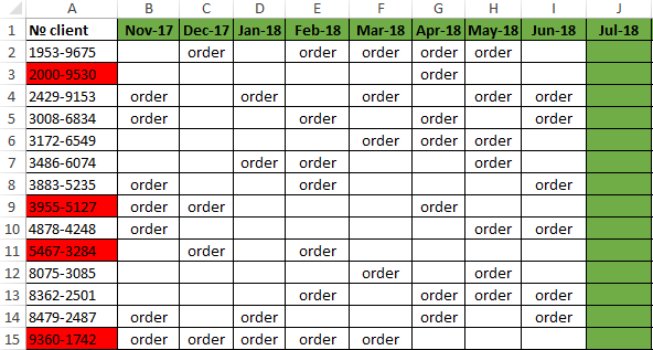
The user to need only to specify, if the customer have made an order in the current month, in the corresponding cell you should enter the text value of «order». The main condition for the allocation: if for 3 months the contractor did not make any order, his number is automatically highlighted in red.
Presented this decision should automate some work processes and to simplify to the visual data analysis.
The automatic filling of the cells with the relevant dates
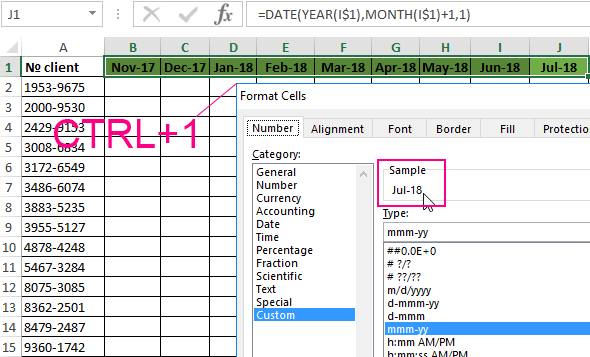
At first, for the register with numbers of customers we will create to the column headers with green and up to date for months that will automatically display to the periods of time. To do this, in the cell B1 you need to enter the following formula:
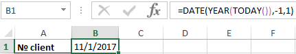
How does the formula work for automatically generating of the outgoing months?
In the picture, the formula returns the period of time passing since the date of writing this article: 17.09.2017. In the first argument in the function DATE is the nested formula that always returns the current year to today’s date thanks to the functions: YEAR and TODAY. In the second argument is the month number (-1). The negative number means that we are interested in what it was a month last time. The example of the conditions for the second argument with the value:
- 1 means the first month (January) in the year that is specified in the first argument;
- 0 – it is 1 month ago;
- -1 – there is 2 months ago from the beginning of the current year (i.e. 01.10.2016).
The last argument-is the day number of the month, which is specified in the second argument. As a result, the DATE function collects all parameters into a single value and the formula returns to the corresponding date.
Next, go to the cell C1 and type the following formula:
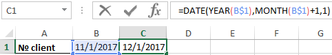
As you can see now the DATE function uses the value from the cell B1 and increases to the month number by 1 in relation to the previous cell. As the result is the 1 – the number of the following month.
Now you need to copy this formula from the cell C1 in the rest of the column headings in the range D1:AY1.
To highlight to the cell range B1:AY1 and select to the tool: «HOME»-«Cells»-«Format Cells» or just to press CTRL+1. In the dialog box that appears, in the tab «Number» in the section «Category» you need to select the option «Custom». In the «Type:» to enter the value: MMM. YY (required the letters in upper register). Because of this, we will get to the cropped display of the date values in the headers of the register, what simplifies to the visual analysis and make it more comfortable due to better readability.
Please note! At the onset of the month of January (D1), the formula automatically changes in the date to the year in the next one.
How to select the column by color in Excel under the terms
Now you need to highlight to the cell by color which respect of the current month. Because of this, we can easily find the column in which you need to enter the actual data for this month. To do this:
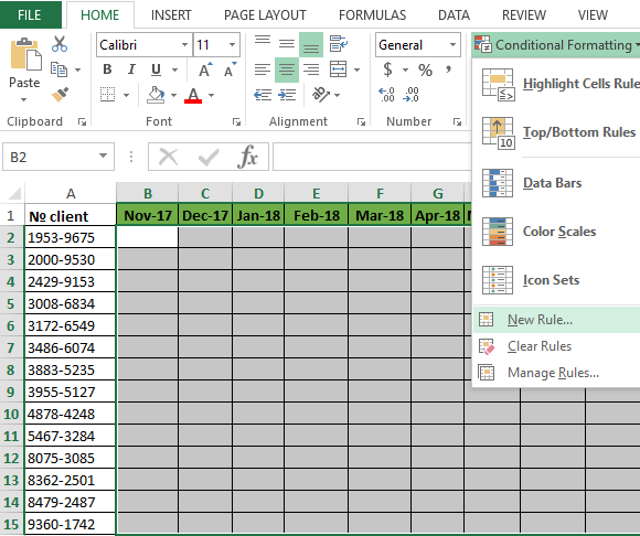
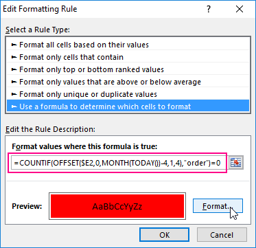
- To select the range of the cells B2:AY15 and select the tool: «HOME» -«Styles» -«Conditional Formatting»-«New Rule». And in the appeared window «New Formatting Rule» you need to select the option: «Use a formula to determine which cells to format»
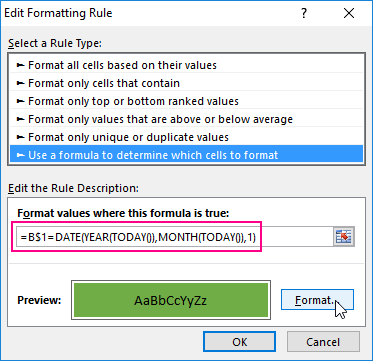
- In the input field to enter the formula:
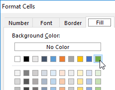
- Click «Format» and indicate on the tab «Fill» in what color (for example green) will be the selected cells of the current month. Then on all Windows for confirmation to click «OK».
The column under the appropriate heading of the register is automatically highlighted in green accordingly to our terms and conditions:
How does the formula highlight of the column color on a condition work?
Due to the fact that before the creation of the conditional formatting rule we have covered all the table data for inputting data of register, the formatting will be active for each cell in the range B2:AY15. The mixed reference in the formula B$1 (absolute address only for rows, but for columns it is relative) determines that the formula will always to refer to the first row of each column.
Automatic highlighting of the column in the condition of the current month
The main condition for the fill by color of the cells: if the range B1:AY1 is the same date that the first day of the current month, then the cells in a column change its colors by specified in conditional formatting.
Please note! In this formula, for the last argument of the function DATE is shown 1, in the same way as for formulas in determining the dates for the column headings of the register.
In our case, is the green filling of the cells. If we open our register in next month, that it has the corresponding column is highlighted in green regardless of the current day.
The table is formatted, now we are filling it with the text value of the «order» in a mixed order of clients for current and past months.
How to highlight the cells in red color according to the condition
Now we need to highlight in red to the cells with the numbers of clients who for 3 months have not made any order. To do this:
- Select the range of the cells A2:A15 (that is, the list of the customer numbers) and select to the tool: «HOME»-«Styles»-«Conditional formatting»-«Create rule». And in the window that appeared «Create a formatting rule» to select the option: «Use the formula for determining which cells to format».
- This time in the input box to enter the formula:
- To click «Format» and specify the red color on the tab «Fill». Then on all Windows click «OK».
- Fill the cells with the text value of «order» as in the picture and look at the result:
The numbers of customers are highlighted in red, if in the row has no have the value «order» in the last three cells for the current month (inclusively).
The analysis of the formula for the highlighting of cells according to the condition
Firstly, we will do by the middle part of our formula. The SHIFT function returns a range reference shifted relative to the basic range of the certain number of rows and columns. The returned reference can be a single cell or a range of cells. Optionally, you can define to the number of returned rows and columns. In our example, the function returns the reference to the cell range for the last 3 months.
The important part for our terms of highlighting in color – is belong to the first argument of the SHIFT function. It determines from which month to start the offset. In this example, there is the cell D2, that is, the beginning of the year – January. Of course for the rest of the cells in the column the row number for the base of the cell will correspond to the line number in what it is located. The following 2 arguments of the SHIFT function to determine how many rows and columns should be done offset. Since the calculations for each customer will carry in the same line, the offset value for the rows we specified is -0.
At the same time for the calculating the value of the third argument (the offset by the columns) we use to the nested formula MONTH(TODAY()), which in accordance with the terms returns to the number of the current month in the current year. From the calculated formula of the month as a number subtract the number 4, that is, in cases November we get the offset by 8 columns. And, for example, for June – there are on 2 columns only.
The last two arguments for the SHIFT function, determine the height (in the number of rows) and width (in the number of columns) of the returned range. In our example, there is the area of the cell with height on 1 row and with width on 4 columns. This range covers to the columns of 3 previous months and the current month.
The first function in the COUNTIF formula checks the condition: how many times in the returned range using the SHIFT function, we can found to the text value «order». If the function returns the value of 0, it means from the client with this number for 3 months there was not any order. And in accordance with our terms and conditions, the cell with number of this client is shown in red fill color.
If we want to register to data for customers, Excel is ideally suited for this purpose. You can easily record in the appropriate categories to the number of ordered goods, as well as the date of implementation of transaction. The problem gradually starts with arising of the data growth.
Download example automatic highlight cells by color.
If so many of them that we need to spend a few minutes looking for a specific position of the register and analysis of the information entered. In this case, it is necessary to add in the table to the register of mechanisms to automate some workflows of the user. And so we did.
Excel has some really amazing functions, but it doesn’t have a function that can sum cell values based on the cell color.
For example, I have the dataset as shown below, and I want to get the sum of all orange and yellow color cells.

Unfortunately, there is no in-built function to do this.
But never say never!
In this tutorial, I will show you three simple techniques you can use to sum by color in Excel.
Let’s dive in!
SUM Cells by Color Using Filter and SUBTOTAL
Let’s start with the easiest one.
Below I have a dataset where I have the employee names and their sales numbers.
And in this dataset, I want to get the sum of all the cells colored in yellow and orange.
While there is no in-built function in Excel to sum values based on cell color, there is a simple workaround that relies on the fact that you can filter cells based on the cell color.
For this method, enter the below formula in cell B17 (or any cell in the same column below the colored cells dataset).
=SUBTOTAL(9,B2:B15)

In the above SUBTOTAL formula, I have used 9 as the first argument, which tells the function that I want to get the sum of the range that is given as the second argument.
But why not just use the SUM formula instead?
This is because when I have the SUBTOTAL formula and I filter the cells to only show those cells that have a specific color in it, the SUBTOTAL formula will show me the sum of visible cells only (something that the SUM formula can not do).
So once you have the SUBTOTAL formula, follow the below steps to get the SUM based on cell color:
- Select any cell in the dataset
- Click the Data tab

- In the Sort and Filter group, click on the Filter icon. This will apply filter to the dataset and you will be able to see the filter icon in the headers
- In the Sales header cell, click on the Filter icon
- Go to the Filter by Color” option
- Select the color based on which you want to filter the dataset.

As soon as you do this, you will notice that the subtotal result changes and it will now only give you the sum of those cells that are visible (which would only be those cells that have the color by which you filtered the dataset).

Similarly, if you filter by some other color in the data set (say orange instead of yellow), the SUBTOTAL function would accordingly adjust and give you the sum of all cells with orange color
Pro Tip: Keyboard shortcut to apply a filter to a dataset is Control + Shift + L (hold the Control and the Shift key, and then press the L key). If using Mac, use Command + Shift + L
SUM Cells by Color Using VBA
I mentioned that there is no inbuilt formula in Excel to sum based on cell color value. However, you can create your own formula to do this using VBA.
With VBA, you can create a custom function that you can keep in the back end, and then use it like any other regular function in the worksheet.
Below is the VBA code that will create that custom function that allows you to sum by color in Excel.
'Code created by Sumit Bansal from https://trumpexcel.com/
'This VBA code created a function that can be used to sum cells based on color
Function SumByColor(SumRange As Range, SumColor As Range)
Dim SumColorValue As Integer
Dim TotalSum As Long
SumColorValue = SumColor.Interior.ColorIndex
Set rCell = SumRange
For Each rCell In SumRange
If rCell.Interior.ColorIndex = SumColorValue Then
TotalSum = TotalSum + rCell.Value
End If
Next rCell
SumByColor = TotalSum
End Function
To use this VBA custom function, you will first have to copy this code and paste it in the back end in the VB editor.
Once done, you’ll be able to use this function in the worksheet.
Below are the steps to add this code to the VB editor.
- Click the Developer tab in the ribbon (if you don’t have the Developer tab visible, click here to learn how to get it)
- Click on the Visual Basic icon. This will open the Visual Basic editor of Excel.

- Click the Insert option in the menu
- Click on Module. This will insert a new module and you will be able to see it in the project explorer (a pane on the left that shows all the objects). If you don’t see the Project Explorer pane, click on View and then click on Project Explorer

- Copy the above VBA code and paste it in the newly inserted Module code window

- Close the VB Editor
Now that you have the code in the back end in excel, you will be able to use the function that we created (SumByColor) in the worksheet.
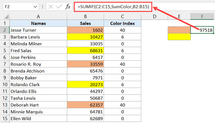
For this function to work, I will need a cell in the worksheet that contains the same color for which I want to get the sum.
In our example, I have done that to cells D2 and D3, where D2 has the yellow color and D3 has the orange color.
Now I can use the below formula in these cells:
=SumByColor($B$2:$B$15,D2)

The above formula takes two arguments:
- The range of cells that have the color that I want to add
- Reference to any cell that contains the color (so that the formula can pick the color index and use that as a condition to add the values)
Note that the formula is dynamic and would automatically update in case you make any changes to the data set (such as changing any value or applying/removing color from some cells). And in case you notice that the formula is not updating, hit the F9 key and it would update.
Since we have used a VBA code in the workbook, it needs to be saved as a macro-enabled workbook (with .XLSM extension).
Pro Tip: If adding cells based on their background color is something you need to do quite often, I recommend you copy and paste this VBA code for the custom formula in the Personal Macro Workbook. This way, that would be available on all your workbooks on your system.
Also read: Filter By Color in Excel
SUM Cells by Color Using GET.CELL
The final method I want to show you include a hidden Excel formula (that not many people know about).
This method uses the GET.CELL function, which can get us the color index value of colored cells.
And once we have the color index value of each cell, we can then use a simple sum if formula to only get the sum of cells with a specific color in it.
It’s not as elegant as the VBA custom function I covered earlier, but if you don’t want to use VBA, then this could be the way to go for you.
GET.CELL is an old Macro 4 function that has been kept in Excel for compatibility reasons, but you won’t find many details about it (as it’s rarely used).
Below I have a dataset where I have colored cells that I want to sum.
For this technique to work, we first need to create a named range that will use the GET.CELL function to give the color value of a colored cell.
Here are the steps to do this:
- Click the Formulas tab in the Ribbon
- In the Defined Names group, click on the ‘Name Manager’

- In the Name Manager dialog box, click on New

- In the ‘New Name dialog box, enter the Name – SumColor

- In the Refers to field, enter the following formula: =GET.CELL(38,$B2)

- Click OK
- Close the Name Manager dialog box
The above steps have created a named range that we can now use in the workbook.
Note: GET.CELL function takes two arguments, the first one is a number that tells the function what information we need, and the second is the cell reference of that cell itself. In this case, I have 38 as the first argument, which would give us the color index value of the referred cell.
Now the second step is to get the color index values of all the colors in column B.
Below are the steps to do this:
- In cell C1, enter the header – Color Index (or anything that you to call it)

- In cell C2, enter the following formula: =SumColor

- Apply the same formula for all the cell in column C (you can use the fill handle or simply copy paste cell C2)

The above steps would give you a value that would represent the color index of the cell in column B (the cell on the left).
SumColor is the named range we created and it uses the GET.CELL function to get the color index value of the cell on the left. You can use this formula in any column, but it should always start from the second cell in that column. For example, instead of column C, you can have this in column H or J, but from the second cells in these columns.
Now that we have a unique number for each color, we can use this to get the SUM of cells based on their color.
Below are the steps to do this:
- In cell E2 and E3, give the cells the color for which you want to get the sum. In my case, I have yellow color in cell E2 and orange in cell E3

- In cell F2, enter the following formula: =SUMIF(C2:C15,SumColor,B2:B15)
- Copy the cell and paste in cell F3 (this could copy the formula as well and adjust the references).

The above steps would give you the sum of all the cells that have the color in the adjacent selling column F.
We have used a SUMIF formula, where it adds all the values in column B, if the color index of the cell on the left (in column F) is the same as that in column C.
While this is definitely a slightly longer way to sum cells by color (as compared with SUBTOTAL or VBA), this gets the work done, and you only need to do this setup once.
Note that while the formula is dynamic, in case you make any changes (such as changing the color cells in column B or removing the color from it), the change might not be reflected instantly in the SUMIF formula. A simple workaround for it would be to go to the cell that has the formula, click the F2 key to get into the airport, and then hit the enter key. This would force the formula to recalculate and you will get the updated result.
So these are three methods you can use to sum by color in Excel. While SUBTOTAL is quite easy and straightforward, I personally like the VBA method better.
I hope you found this tutorial useful!
Other Excel tutorials you may also like:
- Count Characters in a Cell (or Range of Cells) Using Formulas in Excel
- How to Count Colored Cells in Excel
- How to Sort By Color in Excel (in less than 10 seconds)
- How to Apply Formula to Entire Column in Excel
- How to Sum Only Positive or Negative Numbers in Excel (Easy Formula)
- How to SUM values between two dates (using SUMIFS formula)
- How to Combine Duplicate Rows and Sum the Values in Excel
- How to Sum Across Multiple Sheets in Excel? (3D SUM Formula)
- Column
- TECHNOLOGY Q&A
By J. Carlton Collins, CPA
Q. Is there a way to conditionally format Excel so that my formulas automatically display a different font color?
A. You can color—code your formulas using Excel’s conditional formatting tool as follows. Select a single cell (such as cell A1). From the Home tab, select Conditional Formatting, New Rule, and in the resulting New Formatting Rule dialog box, select Use a formula to determine which cells to format. In the resulting Format values where this formula is true box, enter the formula =ISFORMULA(A1) (make sure that no dollar signs appear in the formula). Click the Format button (near the lower—right portion of the dialog box) and select a desired color from the color dropdown box (I have selected green in the example below), and then click OK, OK. (Note: I also selected Bold from the Font style box so the formulas would stand out a little more).

In this example, we have now successfully applied conditional formatting to cell A1, which will display a bold, green font whenever a formula is entered into cell A1. Next, to apply this formatting to the entire worksheet, select cell A1, right—click cell A1, click the Format Painter tool icon, and then click the upper—left corner of the worksheet (in the row and column heading area) to apply this format to the entire worksheet. Thereafter, your entire worksheet will highlight all formulas using a bold, green font, an example of which is pictured below.

You can download this example workbook at carltoncollins.com/formulacolor.xlsx.
About the author
J. Carlton Collins (carlton@asaresearch.com) is a technology consultant, a CPE instructor, and a JofA contributing editor.
Note: Instructions for Microsoft Office in “Technology Q&A” refer to the 2007 through 2016 versions, unless otherwise specified.
Submit a question
Do you have technology questions for this column? Or, after reading an answer, do you have a better solution? Send them to jofatech@aicpa.org. We regret being unable to individually answer all submitted questions.
|January 13, 2016||Filters, SUBTOTAL
If you need to compute the total for certain cells based on their font or fill color, you may have noticed that Excel formulas operate on stored values, not displayed values. That means that functions such as SUM and SUMIFS operate on the underlying cell values and disregard cell formatting, such as font or fill color. This post provides three steps to workaround this issue and compute a total based on fill color.
Objective
Before we get too far, let’s have a look at what we are trying to accomplish.
We have a range of data and selected transactions have been highlighted with a cell fill color, as shown below.
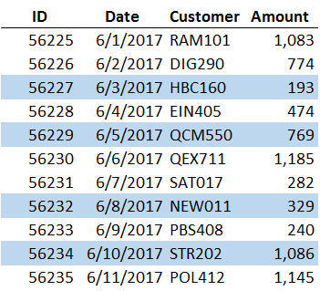
We’ll want to be able to highlight additional rows any time, and we don’t want to rewrite or update our formula when we do. That means our formula range needs to include the amount column and we are precluded from using a formula that picks and chooses each cell (like E10+E12+E15…).
When we try to write a formula that adds up the amount column but includes only the highlighted transactions, we get stuck. Regardless of which summing function we use, we can’t seem to tell Excel to include only the highlighted cells. This is because formulas operate on the underlying stored values and disregard the cell formatting.
So, can we do this? Yes, we can, no worries.
How To
We can accomplish our objective with the help of two Excel items, namely, a filter and a SUBTOTAL function.
Step 1: The filter. We can filter by font or fill color using the built-in filter feature of Excel. To turn on filters, simply select any cell within the data range and then the following Ribbon icon:
- Data > Filter
This will turn on little filter controls, or drop-downs, in the header row. These are shown below.
![]()
With them, we can filter by fill color. Simply pull one down, and then select Filter by Color. A slide-out menu will appear showing the colors used within the data region. When you pick a color, Excel will show those rows and hide the others, as demonstrated below.
Once we have the filter working, we are just about done. All we need to do is write a formula that includes only the visible rows.
Step 2: The blank row. Since we always want our total row to be visible, we don’t want it included within the filter range. To prevent Excel from hiding the total row when applying a filter, we want to skip a row before writing the formula. So, we won’t write our formula in the row immediately under the data range, we’ll leave a blank row in between the last data row and the formula row.
Step 3: SUBTOTAL. Excel has several functions that can add stuff up. To accomplish our objective, we can’t use a standard SUM function because it includes both visible and hidden rows. The SUBTOTAL function on the other hand, includes only visible rows within a filtered region. The trick to using the SUBTOTAL function is to set the first argument to either 9 or 109. Either would work in this case because we want to sum the results and we are using a filter to hide the rows. If our amount column was stored in the range E8:E19, then we would use the following formula in our total row:
=SUBTOTAL(9, E8:E19)
This is pictured below.
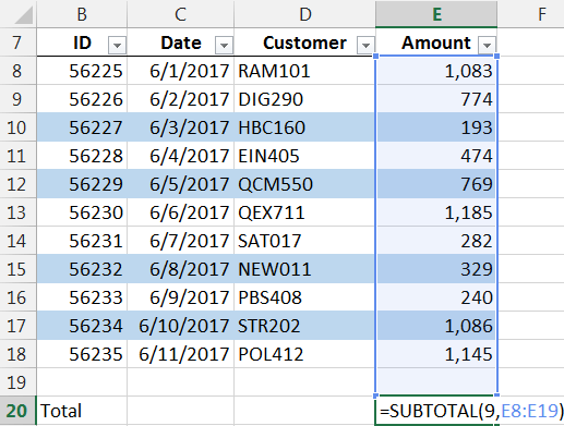
Connecting the dots then…we know we can use the filter to show only the highlighted transactions, we know the blank row between the last data row and the formula will help ensure that our total row is excluded from the filter, and we know the SUBTOTAL function will include only the visible rows within the filtered region. So, will this work? Let’s find out…
Yes, it worked! The total updates from 7,560 (all rows) to 2,377 (highlighted rows)…we have computed a total based on fill color just like we wanted!
If you have any other fun techniques for summing by color, or other suggested uses for filters, please share by posting a comment below…thanks!
Notes
- Download the Excel file: SumByColor
- This technique works if the data is stored in a table as well. Instead of writing the SUBTOTAL formula manually, Excel will add it automatically when we check the Total Row checkbox on the TableTools ribbon tab. Plus, the filter controls will automatically be included in the table’s header row.
- If your total row is being included the the filter (and thus hidden) be sure you have a blank row between the last data row and the formula row and then turn off filters (Data > Filter) and then back on again (Data > Filter).