
You can highlight data in cells by using Fill Color to add or change the background color or pattern of cells. Here’s how:
-
Select the cells you want to highlight.
Tips:
-
To use a different background color for the whole worksheet, click the Select All button. This will hide the gridlines, but you can improve worksheet readability by displaying cell borders around all cells.
-

-
-
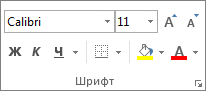
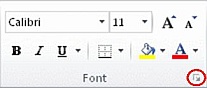
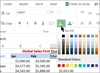
Click Home > the arrow next to Fill Color
, or press Alt+H, H.
-
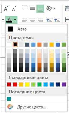
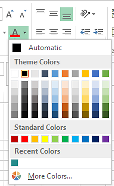
Under Theme Colors or Standard Colors, pick the color you want.
To use a custom color, click More Colors, and then in the Colors dialog box select the color you want.
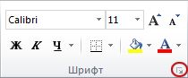
Tip: To apply the most recently selected color, you can just click Fill Color
. You’ll also find up to 10 most recently selected custom colors under Recent Colors.
Apply a pattern or fill effects
When you want something more than a just a solid color fill, try applying a pattern or fill effects.
-
Select the cell or range of cells you want to format.
-
Click Home > Format Cells dialog launcher, or press Ctrl+Shift+F.
-
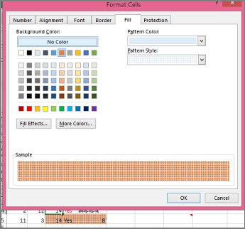
On the Fill tab, under Background Color, pick the color you want.
-
To use a pattern with two colors, pick a color in the Pattern Color box, and then pick a pattern in the Pattern Style box.
To use a pattern with special effects, click Fill Effects, and then pick the options you want.
Tip: In the Sample box, you can preview the background, pattern, and fill effects you selected.
Remove cell colors, patterns, or fill effects
To remove any background colors, patterns, or fill effects from cells, just select the cells. Then click Home > arrow next to Fill Color, and then pick No Fill.
Print cell colors, patterns, or fill effects in color
If print options are set to Black and white or Draft quality — either on purpose, or because the workbook has large or complex worksheets and charts that caused draft mode to be turned on automatically — cells won’t print in color. Here’s how you can fix that:
-
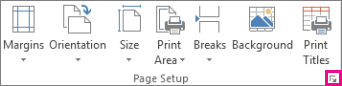
Click Page Layout > Page Setup dialog box launcher.
-
On the Sheet tab, under Print, uncheck the Black and white and Draft quality check boxes.
Note: If you don’t see colors in your worksheet, it may be that you’re working in high contrast mode. If you don’t see colors when you preview before you print, it may be that you don’t have a color printer selected.
If you’d like to highlight text or numbers to make the data more visible, try either changing the font color or add a background color to the cell or range of cells like this:

-
Select the cell or range of cells for which you want to add a fill color.
-
On the Home tab, click Fill Color, and pick the color you want.
Note: Pattern fill effects for background colors are not available for Excel for the web. If you apply any from Excel on your desktop, it won’t appear in the browser.
Remove fill color
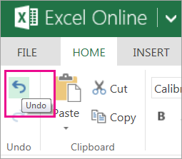
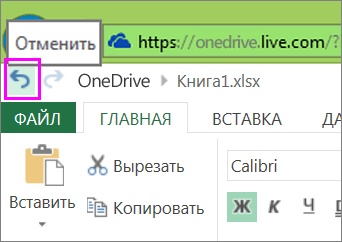
If you decide that you don’t want the fill color immediately after you added it, just click Undo.
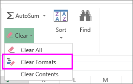
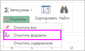
To remove the fill color at a later time, select the cell or cell range you want to change, and click Clear > Clear Formats.
Содержание
- Add or remove a sheet background
- Need more help?
- Добавление и изменение цвета фона ячеек
- Применение узора или способов заливки
- Удаление цвета, узора и способа заливки из ячеек
- Цветная печать ячеек, включая цвет фона, узор и способ заливки
- Удаление цвета заливки
- Дополнительные сведения
- Add or change the background color of cells
- Apply a pattern or fill effects
- Remove cell colors, patterns, or fill effects
- Print cell colors, patterns, or fill effects in color
- Remove fill color
- Need more help?
Add or remove a sheet background
In Microsoft Excel, you can use a picture as a sheet background for display purposes only. A sheet background is not printed, and it is not retained in an individual worksheet or in an item that you save as a Web page.
Because a sheet background is not printed, it cannot be used as a watermark. However, you can mimic a watermark that will be printed by inserting a graphic in a header or footer.
Click the worksheet that you want to display with a sheet background. Make sure that only one worksheet is selected.
On the Page Layout tab, in the Page Setup group, click Background.
Select the picture that you want to use for the sheet background, and then click Insert.
The selected picture is repeated to fill the sheet.
To improve readability, you can hide cell gridlines and apply solid color shading to cells that contain data.
A sheet background is saved with the worksheet data when you save the workbook.
To use a solid color as a sheet background, you can apply cell shading to all cells in the worksheet.
Click the worksheet that is displayed with a sheet background. Make sure that only one worksheet is selected.
On the Page Layout tab, in the Page Setup group, click Delete Background.
Delete Background is available only when a worksheet has a sheet background.
Watermark functionality is not available in Microsoft Excel. However, you can mimic a watermark in one of two ways.
You can display watermark information on every printed page — for example, to indicate that the worksheet data is confidential or a draft copy — by inserting a picture that contains the watermark information in a header or footer. That picture then appears behind the worksheet data, starting at the top or bottom of every page. You can also resize or scale the picture to fill the whole page.
You can also use WordArt on top of the worksheet data to indicate that the data is confidential or a draft copy.
In a drawing program, such as Paintbrush, create a picture that you want to use as a watermark.
In Excel, click the worksheet that you want to display with the watermark.
Note: Make sure that only one worksheet is selected.
On the Insert tab, in the Text group, click Header & Footer.
Under Header, click either the left, center, or right header selection box.
On the Design tab of the Header & Footer Tools, in the Header & Footer Elements group, click Picture  and then find the picture that you want to insert.
Double-click the picture. &[Picture] appears in the header selection box.
Click in the worksheet. The picture you selected will appear in place of &[Picture].
To resize or scale the picture, click the header selection box that contains the picture, click Format Picture in the Header & Footer Elements group, and then, in the Format Picture dialog box, select the options that you want on the Size tab.
Changes to the picture or picture format take effect immediately and cannot be undone.
If you want to add blank space above or below a picture, in the header selection box that contains the picture, click before or after &[Picture], and then press ENTER to start a new line.
To replace a picture in the header section box that contains the picture, select &[Picture], click Picture , and then click Replace.
Before printing, make sure that the header or footer margin has sufficient space for the custom header or footer.
To delete a picture in the header section box that contains the picture, select &[Picture], press DELETE, and then click in the worksheet.
To switch from Page Layout view to Normal view, select any cell, click the View tab, and then, in the Workbook Views group, click Normal.
Click the worksheet location where you want to display the watermark.
On the Insert tab, in the Text group, click WordArt.
Click the WordArt style that you want to use.
For example, use Fill — White, Drop Shadow, Fill — Text 1, Inner Shadow, or Fill — White, Warm Matte Bevel.
Type the text that you want to use for the watermark.
To change the size of the WordArt, do the following:
Click the WordArt.
On the Format tab, in the Size group, in the Shape Height and Shape Width boxes, enter the size that you want . Note that this only changes the size of the box that contains the WordArt.
You can also drag the sizing handles on the WordArt to the size that you want.
Select the text inside the WordArt, and then on the Home tab, in the Font group, select the size you want in the Font Size box.
To add transparency so that you can see more of the worksheet data underneath the WordArt, do the following:
Right-click the WordArt, and click Format Shape.
In the Fill category, under Fill, click Solid fill.
Drag the Transparency slider to the percentage of transparency that you want, or enter the percentage in the Transparency box.
If you want to rotate the WordArt, do the following:
Click the WordArt.
On the Format tab, in the Arrange group, click Rotate.
Click More Rotation Options.
On the Size tab, under Size and rotate, in the Rotation box, enter the degree of rotation that you want.
You can also drag the rotation handle in the direction that you want to rotate the WordArt.
Note: You cannot use WordArt in a header or footer to display it in the background. However, if you create the WordArt in an empty worksheet that does not display gridlines (clear the Gridlines check box in the Show/Hide group on the View tab), you can press PRINT SCREEN to capture the WordArt, and then paste the captured WordArt into a drawing program. You can then insert the picture that you created in the drawing program into a header and footer as described in Use a picture in a header or footer to mimic a watermark.
This feature is not available in Excel for the web.
If you have the Excel desktop application, you can use the Open in Excel button to open the workbook and add a sheet background.
Need more help?
You can always ask an expert in the Excel Tech Community or get support in the Answers community.
Источник
Добавление и изменение цвета фона ячеек
Можно выделить данные в ячейках с помощью кнопки Цвет заливки, чтобы добавить или изменить цвет фона или узор в ячейках. Вот как это сделать:
Выберите ячейки, которые нужно выделить.
Чтобы использовать другой цвет фона для всего таблицы, нажмите кнопку Выбрать все. При этом линии сетки будут скроются, но вы сможете улучшить читаемость, отобразив границы ячеек вокруг всех ячеек.
Щелкните Главная > стрелку рядом с кнопкой Цвет заливки  или нажмите клавиши ALT+H, H.
Выберите нужный цвет в группе Цвета темы или Стандартные цвета.
Чтобы использовать дополнительный цвет, выберите команду Другие цвета, а затем в диалоговом окне Цвета выберите нужный цвет.
Совет: Чтобы применить последний выбранный цвет, достаточно нажать кнопку Цвет заливки . Кроме того, в группе Последние цвета доступны до 10 цветов, которые вы выбирали в последнее время.
Применение узора или способов заливки
Если вас не устраивает сплошная заливка цветом, попробуйте применить узор или один из доступных способов заливки.
Выделите ячейку или диапазон ячеек, которые нужно отформатировать.
На вкладке Главная нажмите кнопку вызова диалогового окна Формат ячеек или просто нажмите клавиши CTRL+SHIFT+F.
На вкладке Заливка выберите в разделе Цвет фона нужный цвет.
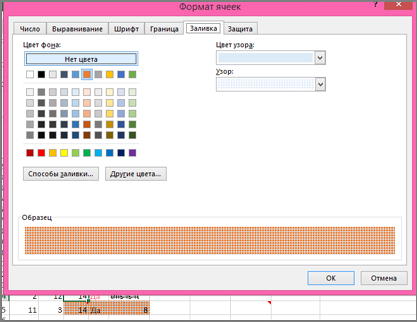
Чтобы использовать двухцветный узор, выберите цвет в поле Цвет узора, а затем выберите сам узор в поле Узор.
Чтобы создать узор со специальными эффектами, нажмите кнопку Способы заливки и выберите нужные параметры.
Совет: В поле Образец можно просмотреть выбранный фон, узор и способ заливки.
Удаление цвета, узора и способа заливки из ячеек
Чтобы удалить все цвета фона, узоры и способы заливки, просто выделите ячейки. На вкладке Главная нажмите стрелку рядом с кнопкой Цвет заливки и выберите пункт Нет заливки.
Цветная печать ячеек, включая цвет фона, узор и способ заливки
Если заданы параметры печати черно-белая или черновая (преднамеренно или потому, что книга содержит большие или сложные листы и диаграммы, вследствие чего черновой режим включается автоматически), заливку ячеек невозможно вывести на печать в цвете. Вот как можно это исправить:
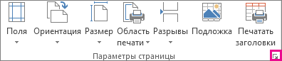
Откройте вкладку Разметка страницы и нажмите кнопку вызова диалогового окна Параметры страницы.
На вкладке Лист в группе Печать снимите флажки черно-белая и черновая.
Примечание: Если цвета на листе не отображаются, возможно, выбран высококонтрастный режим. Если цвета не отображаются при предварительном просмотре, возможно, не выбран цветной принтер.
Если вы хотите выделить текст или числа, чтобы сделать данные более заметными, попробуйте изменить цвет шрифта или добавить цвет фона к ячейке или диапазону ячеек.
Вы ячейка или диапазон ячеек, для которых нужно добавить цвет заливки.
На вкладке Главная нажмите кнопку Цвет заливкии выберите нужный цвет.
Примечание: Эффекты узорной заливки для цветов фона недоступны для Excel в Интернете. Если применить любой из Excel на компьютере, он не будет отображаться в браузере.
Удаление цвета заливки
Если вы решите, что цвет заливки не нужен сразу после его вжатия, просто нажмите кнопку Отменить .
Чтобы позже удалить цвет заливки, вы выберите ячейку или диапазон ячеок, которые вы хотите изменить, и нажмите кнопку Очистить > Очистить форматы.
Дополнительные сведения
Вы всегда можете задать вопрос специалисту Excel Tech Community или попросить помощи в сообществе Answers community.
Источник
Add or change the background color of cells
You can highlight data in cells by using Fill Color to add or change the background color or pattern of cells. Here’s how:
Select the cells you want to highlight.
To use a different background color for the whole worksheet, click the Select All button. This will hide the gridlines, but you can improve worksheet readability by displaying cell borders around all cells.

Click Home > the arrow next to Fill Color  , or press Alt+H, H.
Under Theme Colors or Standard Colors, pick the color you want.
To use a custom color, click More Colors, and then in the Colors dialog box select the color you want.
Tip: To apply the most recently selected color, you can just click Fill Color . You’ll also find up to 10 most recently selected custom colors under Recent Colors.
Apply a pattern or fill effects
When you want something more than a just a solid color fill, try applying a pattern or fill effects.
Select the cell or range of cells you want to format.
Click Home > Format Cells dialog launcher, or press Ctrl+Shift+F.
On the Fill tab, under Background Color, pick the color you want.
To use a pattern with two colors, pick a color in the Pattern Color box, and then pick a pattern in the Pattern Style box.
To use a pattern with special effects, click Fill Effects, and then pick the options you want.
Tip: In the Sample box, you can preview the background, pattern, and fill effects you selected.
Remove cell colors, patterns, or fill effects
To remove any background colors, patterns, or fill effects from cells, just select the cells. Then click Home > arrow next to Fill Color, and then pick No Fill.
Print cell colors, patterns, or fill effects in color
If print options are set to Black and white or Draft quality — either on purpose, or because the workbook has large or complex worksheets and charts that caused draft mode to be turned on automatically — cells won’t print in color. Here’s how you can fix that:
Click Page Layout > Page Setup dialog box launcher.
On the Sheet tab, under Print, uncheck the Black and white and Draft quality check boxes.
Note: If you don’t see colors in your worksheet, it may be that you’re working in high contrast mode. If you don’t see colors when you preview before you print, it may be that you don’t have a color printer selected.
If you’d like to highlight text or numbers to make the data more visible, try either changing the font color or add a background color to the cell or range of cells like this:
Select the cell or range of cells for which you want to add a fill color.
On the Home tab, click Fill Color, and pick the color you want.
Note: Pattern fill effects for background colors are not available for Excel for the web. If you apply any from Excel on your desktop, it won’t appear in the browser.
Remove fill color
If you decide that you don’t want the fill color immediately after you added it, just click Undo .
To remove the fill color at a later time, select the cell or cell range you want to change, and click Clear > Clear Formats.
Need more help?
You can always ask an expert in the Excel Tech Community or get support in the Answers community.
Источник
Home / Excel Basics / Apply Background Color to a Cell or the Entire Sheet in Excel
As you know, White is the default background color in Excel and most of the time to highlight a cell or a range of cells, users prefer to apply the background color to the cells.
In Excel, background color can be applied using several ways, like by using the “Fill Color” option or by applying different types of conditions using the “Conditional Formatting” option and many more.
The background color once applied to the cells or the sheet using the “Fill Color” option will not change with the change in the value of the cells, on the other hand using the “Conditional Formatting” option, the color of the cells changes with the change in cell value based on the conditions applied.
We have mentioned some quick and simple steps for you to apply background color in Excel.
Apply Background Color Using Fill Color Option
- First, select the cell or range of cells or the entire sheet to apply the background color to the cell or range of cells or the entire sheet respectively.
- After that, go to the “Home” tab and then click on the “Fill Color” drop-down arrow and select the color you want to apply.

- Once you select the color, you will get your selected cells or cells range or the entire sheet highlighted with the selected color.

Apply Background Color Based on the Cell Values Using Conditional Formatting
Using conditional formatting users can apply background colors to the cells based on one or multiple conditions at the same time, like value greater than, value less than, values equal to, duplicate values, text in the cell, etc.
And whenever the cell value gets updated, the color of the cell changes automatically according to the conditions specified.
- First, select the entire sheet or a range of cells where you want to apply the background color formatting, and then go to the “Home” tab.
- After that, click on the “Conditional Formatting” drop-down arrow and then click on the “Highlight Cells Rules” and then click on the “More Rules” option.

- Once you click on “More Rules”, you will get the “New Formatting Rule” dialog box opened.

- Now, select the rule type “Format only cells that contain” and then select the formatting condition you want to apply then enter the value and then click on the “Format” button.

- Now in the “Format Cells” dialog box, select the “Fill” header and then choose the color you want to apply and then click OK.

- Once you click OK, you will get back to the “New Formatting Rule” dialog box, where you can now see the preview of the selected color.
- In the end, click OK.

- At this point, you will get the cells of your selected range highlighted with the background color based on the condition applied.


In the above example, we have selected the condition of “Greater than or equal to” with a base value of “10000” and color as green therefore all the cells having a value of 10000 or more got highlighted with the green background color.
To apply more color formatting conditions on the same range, users need to follow the same steps and just need to apply the second condition parallel to the first one that we have created above.
You can now see the two different colors based on the two conditions which we had applied.
And in the same way, you can apply more conditions to the same range like highlighting the background color with the cells equal to zero (0), and in that case, you have to apply the new condition “Equal to” with the value entered as zero (0).
Where you will get the cells with value zero highlighted with the background color which you will select while applying the condition.
Apply Background Color to the Special Cells Using Conditional Formatting
Special cells here refer to the cells that are blank or empty with no data or the cells with formula errors.
- First, select the cells range or the entire table or the entire sheet if you want to apply background color to the special cells from a particular range of cells or the entire table or entire sheet respectively.

- After that, go to the “Conditional Formatting” and then click on “New Rule” and open the “New Formatting Rule” dialog box.
- Now, click on the left side drop-down arrow and select the “Blanks” or “Errors” option to apply background color to the blank cells or the cells with errors.

- Once you are done with the selection of the format cell type as “Blank” or any other type based on within which cells you want to apply color then click on the “Format” button and select the color type.
- In the end, click OK.

- At this point, you will get the cells of your selected range or table or sheets highlighted with the color based on the condition applied.


Apply Background Color Using Cell Styles
- First, select the cells range or the entire table or the entire sheet if you want to apply background color to the special cells from a particular range of cells or the entire table or entire sheet respectively.
- After that, go to the “Home” tab, then click on the “Cell Styles” icon, and then select the background color style you want to apply.
- In this example, we have selected the “Neutral” color for the selected table.

- Once you select the color, you will get your selected cells or range or table or sheet applied with that color.


In Excel, there are several ways to apply background color to the cell or the entire sheet, but all depends on your requirement.
If you want the color once applied to not change with any change in the cell value, then you can simply use the “Fill Color” or Format Cells” or Cell Styles” option.
But if you want your cell colors dynamic means that color will change automatically with the change in the cell value and based on the conditions applied, you can use the “Conditional Formatting” option in this case.
In this article, you will learn how to change the background color of a cell in Excel and Google Sheets.
Change the Background Color
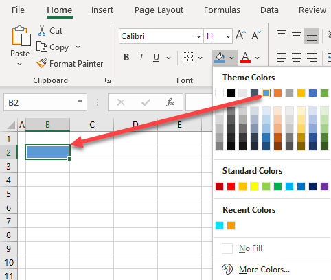
To change a cell’s background color, click on the cell (B2, in this example).
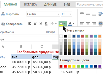
Then in the Ribbon, go to Home > Fill Color and choose a color (e.g., Blue, Accent 1, shown below).
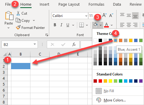
The background of cell B2 is now filled with the color Blue, Accent 1. As you move the cursor over colors, the cell color will change, but you have to click on the color to confirm the change.
To clear the color of the cell, click again on cell B2 and in the Ribbon, go to Home > Fill Color > No Fill.
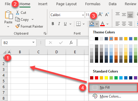
Now the background color of B2 is removed.
Color Palette
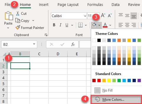
Apart from the standard colors offered in the Fill Color menu, there are more colors from the palette to choose from.
1. Select the cell and in the Ribbon, go to Home > Fill Color > More Colors.
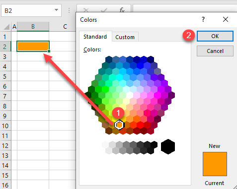
2. In the pop-up screen, choose a color and click OK.
Color Codes
There’s also the option to use the RGB color code or Hexadecimal to fill the cell background.
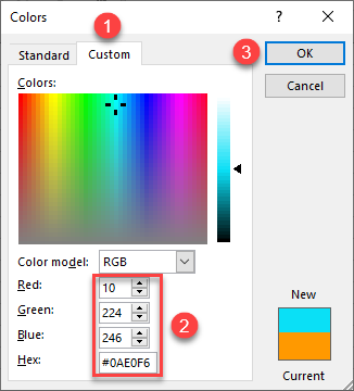
In the Colors window, (1) go to the Custom tab, (2) enter the RBG or Hex code, and (3) click OK.
You can also click on any color, and the RBG and Hex codes will be populated based on the chosen color.
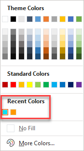
All colors added through the More Colors option will be added as Recent Colors in the Fill Color menu and can easily be used again.
Change the Cell Background Color in Google Sheets
To change the cell background color in Google Sheets, (1) select the cell and in the Toolbar, (2) go to Fill Color and (3) choose the color (e.g., orange, shown below).
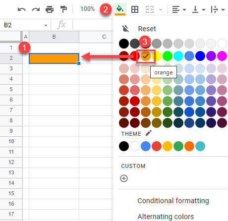
As a result, the cell B2 background is now filled with orange.
To clear the cell background, (1) select the cell again, and in the Toolbar, (2) go to Fill Color and (3) click Reset.
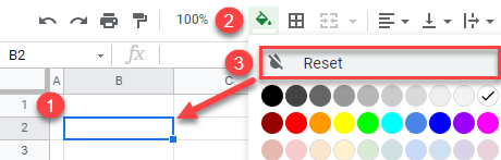
After this, cell B2 has no background color.
Hex Code
As in Excel, you can use the Hex code to select an additional color.
1. Select the cell and in the Toolbar, go to Fill Color. Then click the plus sign under Custom.
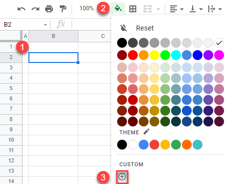
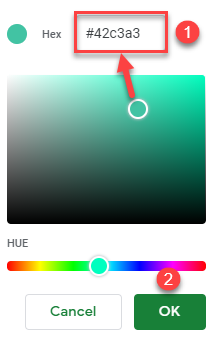
2. In the pop-up window, enter the Hex color code and click OK.
If you don’t know the hex code, you can choose a color on the palette, and the hex code will be populated automatically.
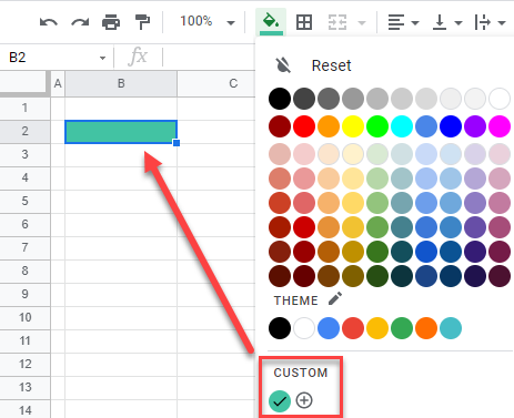
As a result, the cell B2 background is filled with the custom color. If you go back to the Fill Color menu, this new color is added under Custom colors and can be reused anytime.
 Please Note:
This article is written for users of the following Microsoft Excel versions: 2007, 2010, 2013, 2016, 2019, and Excel in Microsoft 365. If you are using an earlier version (Excel 2003 or earlier), this tip may not work for you. For a version of this tip written specifically for earlier versions of Excel, click here: Changing Excel’s Background Color.
![]()
Written by Allen Wyatt (last updated September 7, 2019)
This tip applies to Excel 2007, 2010, 2013, 2016, 2019, and Excel in Microsoft 365
The standard background color in Excel is white. You may, at some time, want to change the background color to something else, such as a light grey. Unfortunately, there is no way to change the background color; it is not a configurable option in Excel. There are a few things you can try as workarounds, however.
One approach involves selecting all the cells in the worksheet and applying a fill color to the cells. If you don’t want the color to print, then you simply need to select all the cells and remove the fill color. This could be automated by using a macro to do the color removal, printing, and re-application.
There are drawbacks to such an approach, however. First, the colors used to fill the cells could interfere with the successful application of conditional formatting, if the conditional formatting involves the use of fill colors. (Conditional formatting applied to font specifications shouldn’t be a problem.)
Another option is to create, in your favorite graphics program, a small rectangle that matches the color you want used for your background. Save the small rectangle as a graphics file, using the PNG file format. Then, within Excel, follow these steps:
- Display the Page Layout tab of the ribbon.
- Click the Background tool, in the Page Setup group. Excel 2007 and Excel 2010 display the Sheet Background dialog box. In Excel 2013 and later versions you see the Insert Pictures screen in which you should click the Browse link at the right of the From a File option. You’ll then see the Sheet Background dialog box. (See Figure 1.)
- Use the controls in the dialog box to locate and select the graphic image you created (the small rectangle of color).
- Click the Insert button.
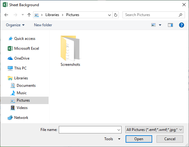
Figure 1. The Sheet Background dialog box.
The graphic image is placed in the background and repeated over and over again so that it fills the entire background. The benefit to this approach is that it doesn’t affect any conditional formatting and the background image won’t print.
Speaking of conditional formatting, if you aren’t using conditional formatting for any purpose in a worksheet, you could use it to create your background. In a blank area of your workbook, define a cell that contains the value True. Then select your worksheet that you want to have the background color and use a conditional format to define that color. The format can look at the cell you defined, and if it is True, then the color is applied. If the cell is not True, then the color is not applied. This allows you to turn the background color on or off (for printing) by changing the value of a single cell.
You could also define styles for use in your worksheet. Define a style that has the desired background color, and another that does not. You can then apply the colored style when editing and the non-colored style when preparing to print.
ExcelTips is your source for cost-effective Microsoft Excel training.
This tip (6121) applies to Microsoft Excel 2007, 2010, 2013, 2016, 2019, and Excel in Microsoft 365. You can find a version of this tip for the older menu interface of Excel here: Changing Excel’s Background Color.
Author Bio
With more than 50 non-fiction books and numerous magazine articles to his credit, Allen Wyatt is an internationally recognized author. He is president of Sharon Parq Associates, a computer and publishing services company. Learn more about Allen…
MORE FROM ALLEN
Two Page Numbers per Physical Page
If your document has two mini pages on one page, inserting page numbers in Word, so that each mini page has its own …
Discover More
Backing Up Quick Access Toolbars
The Quick Access Toolbar is a place where you can easily put your customizations. If you want to back up that toolbar …
Discover More
Using Multiple References to the Same Footnote
Do you want to have multiple footnote references to the same actual footnote in a document? The easiest way to do this is …
Discover More

Color in Excel (Table of Contents)
- Introduction to Color in Excel
- Ways to Change Background Color
Introduction to Color in Excel
Colors are generally used to highlight a group of cells in Excel. The excel contains the index of 56 colors. By using conditional formatting, we can put some conditions and apply different colors for different conditions if we want to change the background color of the cell in Excel. We usually select the cells and click the Fill color option; then, the background color will get changed if we want to change the cell’s background colour with the cell automatically.
Ways to Change Background Color
There are two ways to change the background color.
You can download this Color Excel Template here – Color Excel Template
1. Change the color of the cell based on the current value
- Here the background color of the cell changes when the cell value in the Excel changes.
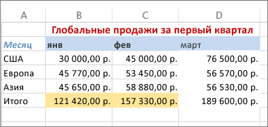
- For example, we have taken the following dataset. we want the USD Amount greater than 10,000 as blue color and remaining red color.

- Select the range of the cells which we want to change. Then go to the Home tab, go to the styles and select the conditional formatting.

- Now click on the new rules.
- A dialog appears stating the selection of the row. Select the format of the cells based on the cell value.

- Now give the range of values which are greater than 10,000 and select the color as blue color.


- Now click on the format option.
- A color box appears and makes the Pattern Color as Automatic, so Select color as blue and click on OK.

- We can observe that the sample option is blue because we have selected the blue color.

- We can observe the selected color in the format option. And click the Ok option.

- Now we can use the same procedure for selecting the color for less value. A dialog appears stating the selection of the row. Select the format of the cells based on the cell value. A dialog appears stating the selection of the row. Select the format of the cells based on the cell value. Now give the range of values which are less than 10,000 and select the color as red color.

- The color box appears and makes the pattern as automatic and Select color like blue and click OK.
- The output will be as follows.

2. Change the background color of special cells
- This is another way of color the background of the particular cell. First, go to the home tab, then select the conditional formatting.

- Select the new rules.
- The formatting dialog box appears to click on the cells which need to format, which is at the end of the dialog box.

- Click on the arrow option at the right end.
- Write the new formatting rule using the keyword Is Blank condition. This Is Blank is used to highlighting the background cells which are empty.

- Click on the Format option. And select the blue color.

- Click on the Ok button.

- The output will be as follows.

3. Sort the Excel by it Color
- Sorting is one of the methods to select a particular color. First, select the cells, right-click on them, select the sort option, and then select the highest value by color.

- Click the ok button.
- And Filter the color by its color.


- And the output will be as follows.
Change the cell color based on the current value.
- First, go to the home tab, select the Find and select option, and select the Find option.
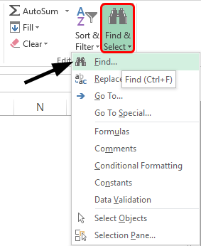
- Select the value which we want to select. Click on the Find all option.
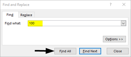
- Click on the values range which we want the cells we want to highlight.
- Click on the Select by value option. And select the Greater in the list.
- Click on the range of the cells we want to highlight. Click on the select option.
- Now select the color as blue for the greater value.
- And the output will be as follows.
Conditional Formatting in Excel
- Conditional formatting is generally used to color data bars and icons in the cells.
- To do the conditional formatting in Excel, first, we take the required data set.
- Then go to the Home tab and select the conditional formatting option ad put the desired rule which we want to specify, and mention the color which we want to give to the cells of the particular condition.
- Then a dialog box appears on the screen then simply gives the values we want a particular condition so that the color will be applied successfully.
- Now select the formatting styles from the drop-down. Here we select the color for the condition. Then click the OK. The conditional formatting will be applied to all the cells at a time. This is one way of adding colors to the cells.
Things to Remember About Color in Excel
- The colors in excel play a major role in highlighting a particular range of cells.
- Here we generally use the two approaches like make the background color cells based on the value, and another way is to change the background of special cells.
- The excel contains the index of 56 colors. By using conditional formatting, we can put some conditions and apply different colors for different conditions.
- We can also sort the colors based on the colors.
- We can highlight the empty cells with the colors.
- Through cells, we can highlight the greater values and the lower value with different colors.
Recommended Articles
This has been a guide to Color in Excel. Here we discuss How to use Color in Excel along with practical examples and a downloadable excel template. You can also go through our other suggested articles –
- Alternate Row Color Excel
- Excel Sum by Color
- Count Colored Cells In Excel
- Excel Sort by color
Change Background Color of Cell Range in Excel VBA
Description:
It is an interesting feature in excel, we can change background color of Cell, Range in Excel VBA. Specially, while preparing reports or dashboards, we change the backgrounds to make it clean and get the professional look to our projects.
Change Background Color of Cell Range in Excel VBA – Solution(s):
![]()
We can use Interior.Color OR Interior.ColorIndex properties of a Rage/Cell to change the background colors.
Change Background Color of Cell Range in Excel VBA – Examples
The following examples will show you how to change the background or interior color in Excel using VBA.
Example 1
In this Example below I am changing the Range B3 Background Color using Cell Object
Sub sbRangeFillColorExample1()

'Using Cell Object
Cells(3, 2).Interior.ColorIndex = 5 ' 5 indicates Blue Color

End Sub
Example 2
In this Example below I am changing the Range B3 Background Color using Range Object
Sub sbRangeFillColorExample2()

'Using Range Object
Range("B3").Interior.ColorIndex = 5

End Sub
Example 3
We can also use RGB color format, instead of ColorIndex. See the following example:
Sub sbRangeFillColorExample3()
'Using Cell Object
Cells(3, 2).Interior.Color = RGB(0, 0, 250)

'Using Range Object
Range("B3").Interior.Color = RGB(0, 0, 250)

End Sub
Example 4
The following example will apply all the colorIndex form 1 to 55 in Activesheet.
Sub sbPrintColorIndexColors()
Dim iCntr

For iCntr = 1 To 56
    Cells(iCntr, 1).Interior.ColorIndex = iCntr
    Cells(iCntr, 1) = iCntr
Next iCntr

End Sub
Instructions:
- Open an excel workbook
- Press Alt+F11 to open VBA Editor
- Insert a new module from Insert menu
- Copy the above code and Paste in the code window
- Save the file as macro enabled workbook
- Press F5 to execute the procedure
- You can see the interior colors are changing as per our code
Change Background Color of Cell Range in Excel VBA – Download: Example File
Here is the sample screen-shot of the example file.
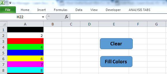
Download the file and explore how to change the interior or background colors in Excel using VBA.
ANALYSIS TABS – ColorIndex
A Powerful & Multi-purpose Templates for project management. Now seamlessly manage your projects, tasks, meetings, presentations, teams, customers, stakeholders and time. This page describes all the amazing new features and options that come with our premium templates.
Save Up to 85% LIMITED TIME OFFER

All-in-One Pack
120+ Project Management Templates
Essential Pack
50+ Project Management Templates
Excel Pack
50+ Excel PM Templates
PowerPoint Pack
50+ Excel PM Templates
MS Word Pack
25+ Word PM Templates
Ultimate Project Management Template
Ultimate Resource Management Template
Project Portfolio Management Templates
Related Posts
VBA Reference
Effortlessly
Manage Your Projects
120+ Project Management Templates
Seamlessly manage your projects with our powerful & multi-purpose templates for project management.
120+ PM Templates Includes:
3 Comments
-
Harbinder Singh
April 13, 2017 at 12:23 PM — Replyneed help in excel
In company there are 10000 employee and all having duty in A shift, B shift, C shift. Each shift of 08 hrs
i have to find those employee who work continuous 10 days or more then 10 days
please help me to find the solution using VB macro in excel or any other way to find from huge no of data in excel
Kindly provide me the solution.
-
RandomOne
May 23, 2017 at 5:46 AM — ReplyHarbinder Singh
its dependes of your database, can check with a vba code for filter based on the criteria, select the range and then color it,
Regards! -
Ken Schleede
July 10, 2019 at 6:44 AM — ReplyThanks! This is excellent. It allows me to control the colors much more reliably than conditional formatting.
Effectively Manage Your
Projects and Resources
ANALYSISTABS.COM provides free and premium project management tools, templates and dashboards for effectively managing the projects and analyzing the data.
We’re a crew of professionals expertise in Excel VBA, Business Analysis, Project Management. We’re Sharing our map to Project success with innovative tools, templates, tutorials and tips.
Project Management
Excel VBA
Download Free Excel 2007, 2010, 2013 Add-in for Creating Innovative Dashboards, Tools for Data Mining, Analysis, Visualization. Learn VBA for MS Excel, Word, PowerPoint, Access, Outlook to develop applications for retail, insurance, banking, finance, telecom, healthcare domains.
Page load link
Go to Top
Setting the Color property alone will guarantee an exact match. Excel 2003 can only handle 56 colors at once. The good news is that you can assign any rgb value at all to those 56 slots (which are called ColorIndexs). When you set a cell’s color using the Color property this causes Excel to use the nearest «ColorIndex». Example: Setting a cell to RGB 10,20,50 (or 3281930) will actually cause it to be set to color index 56 which is 51,51,51 (or 3355443).
If you want to be assured you got an exact match, you need to change a ColorIndex to the RGB value you want and then change the Cell’s ColorIndex to said value. However you should be aware that by changing the value of a color index you change the color of all cells already using that color within the workbook. To give an example, Red is ColorIndex 3. So any cell you made Red you actually made ColorIndex 3. And if you redefine ColorIndex 3 to be say, purple, then your cell will indeed be made purple, but all other red cells in the workbook will also be changed to purple.
There are several strategies to deal with this. One way is to choose an index not yet in use, or just one that you think will not be likely to be used. Another way is to change the RGB value of the nearest ColorIndex so your change will be subtle. The code I have posted below takes this approach. Taking advantage of the knowledge that the nearest ColorIndex is assigned, it assigns the RGB value directly to the cell (thereby yielding the nearest color) and then assigns the RGB value to that index.
Sub Example()
    Dim lngColor As Long
    lngColor = RGB(10, 20, 50)
    With Range("A1").Interior
        .Color = lngColor
        ActiveWorkbook.Colors(.ColorIndex) = lngColor
    End With
End Sub