
Adding a color to alternate rows or columns (often called color banding) can make the data in your worksheet easier to scan. To format alternate rows or columns, you can quickly apply a preset table format. By using this method, alternate row or column shading is automatically applied when you add rows and columns.
Here’s how:
-
Select the range of cells that you want to format.
-
Click Home > Format as Table.
-
Pick a table style that has alternate row shading.
-
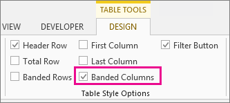
To change the shading from rows to columns, select the table, click Design, and then uncheck the Banded Rows box and check the Banded Columns box.

Tip: If you want to keep a banded table style without the table functionality, you can convert the table to a data range. Color banding won’t automatically continue as you add more rows or columns but you can copy alternate color formats to new rows by using Format Painter.
Use conditional formatting to apply banded rows or columns
You can also use a conditional formatting rule to apply different formatting to specific rows or columns.
Here’s how:
-
On the worksheet, do one of the following:
-
To apply the shading to a specific range of cells, select the cells you want to format.
-
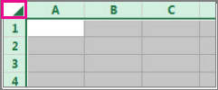
To apply the shading to the whole worksheet, click the Select All button.
-
-
Click Home > Conditional Formatting > New Rule.
-
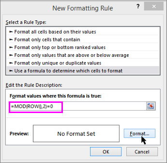
In the Select a Rule Type box, click Use a formula to determine which cells to format.
-
To apply color to alternate rows, in the Format values where this formula is true box, type the formula =MOD(ROW(),2)=0.
To apply color to alternate columns, type this formula: =MOD(COLUMN(),2)=0.
These formulas determine whether a row or column is even or odd numbered, and then applies the color accordingly.
-
Click Format.
-
In the Format Cells box, click Fill.
-
Pick a color and click OK.
-
You can preview your choice under Sample and click OK or pick another color.
Tips:
-
To edit the conditional formatting rule, click one of the cells that has the rule applied, click Home > Conditional Formatting > Manage Rules > Edit Rule, and then make your changes.
-
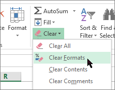
To clear conditional formatting from cells, select them, click Home > Clear, and pick Clear Formats.
-
To copy conditional formatting to other cells, click one of the cells that has the rule applied, click Home > Format Painter
, and then click the cells you want to format.
-
Need more help?
Want more options?
Explore subscription benefits, browse training courses, learn how to secure your device, and more.
Communities help you ask and answer questions, give feedback, and hear from experts with rich knowledge.
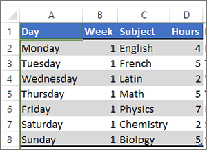
In this lesson we will learn how to change the color of a table in Excel. For this, we will initialize the original table from the previous lesson by formatting the background and cell borders.
Immediately go over to practice. We select the whole table A1:D4.
On the «Home» tab, click on the «Borders» tool, which is located in the «Font» section. From the drop-down list, select the option «All borders».
Now again in the same list, select the option «Thick outer border». Next, select the range A1:D1. In the same section of the tools, click on «Fill color» and point to «Dark Blue». Next, in the «Text color» tool, point «White».
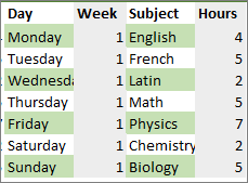
The example of changing the color of tables
The pictures show the process of changing the boundaries in practice:
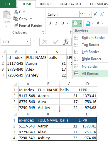
You can also change the color of a table in Excel using the more functional tool.
Select again the entire table A1:D4. Press the hotkey combination CTRL + 1 or CTRL + SHIFT + F. The multifunction dialog box «Format Cells» will appear.
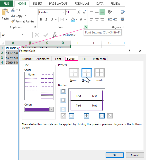
First go to the «Border» tab. In the «Presets» toolbar of this tab, click the «Inside» button. Now in the line type section, select the thickest line (second from the bottom in the right column). If necessary, set the color for the borders of the table below. Then go back to the «All» section and click on the «Outline» button. To confirm the border formatting settings, click OK.
Also we can make a colors text. Select the headings of the original table A1:D1. Open the «Format Cells» window. At present go to the «Font» tab and in the text color field select «Yellow». To change the color of the selected cell in Excel, click the «Fill» tab and click on «Black». To confirm the change of the format of the cells, click OK. Pasting cells in Excel allows you to select a row or column by color.
As you can see in the «Format Cells» window there are multiplicity of tools, that expand the possibilities of formatting data.
The helpful advice! Format the data in the last place: so you will save your working time.
The formatting opens up wide possibilities for data exposure. There are the changing fonts and sizes of text, setting background colors and patterns, paint border colors and select the type of their lines, etc. But if you slightly overdo with the color change a little, the Excel sheet becomes colorful and unreadable.
Содержание
- Change the color of the table in Excel
- The example of changing the color of tables
- Apply shading to alternate rows or columns in a worksheet
- Need more help?
- Apply color to alternate rows or columns
- Use conditional formatting to apply banded rows or columns
- Format an Excel table
- Choose a table style
- Choose table style options to format the table elements
- Need more help?
Change the color of the table in Excel
In this lesson we will learn how to change the color of a table in Excel. For this, we will initialize the original table from the previous lesson by formatting the background and cell borders.
Immediately go over to practice. We select the whole table A1:D4.
On the «Home» tab, click on the «Borders» tool, which is located in the «Font» section. From the drop-down list, select the option «All borders».
Now again in the same list, select the option «Thick outer border». Next, select the range A1:D1. In the same section of the tools, click on «Fill color» and point to «Dark Blue». Next, in the «Text color» tool, point «White».
The example of changing the color of tables
The pictures show the process of changing the boundaries in practice:
You can also change the color of a table in Excel using the more functional tool.
Select again the entire table A1:D4. Press the hotkey combination CTRL + 1 or CTRL + SHIFT + F. The multifunction dialog box «Format Cells» will appear.
First go to the «Border» tab. In the «Presets» toolbar of this tab, click the «Inside» button. Now in the line type section, select the thickest line (second from the bottom in the right column). If necessary, set the color for the borders of the table below. Then go back to the «All» section and click on the «Outline» button. To confirm the border formatting settings, click OK.
Also we can make a colors text. Select the headings of the original table A1:D1. Open the «Format Cells» window. At present go to the «Font» tab and in the text color field select «Yellow». To change the color of the selected cell in Excel, click the «Fill» tab and click on «Black». To confirm the change of the format of the cells, click OK. Pasting cells in Excel allows you to select a row or column by color.
As you can see in the «Format Cells» window there are multiplicity of tools, that expand the possibilities of formatting data.
The helpful advice! Format the data in the last place: so you will save your working time.
The formatting opens up wide possibilities for data exposure. There are the changing fonts and sizes of text, setting background colors and patterns, paint border colors and select the type of their lines, etc. But if you slightly overdo with the color change a little, the Excel sheet becomes colorful and unreadable.
Источник
Apply shading to alternate rows or columns in a worksheet
This article shows you how to automatically apply shading to every other row or column in a worksheet.
There are two ways to apply shading to alternate rows or columns —you can apply the shading by using a simple conditional formatting formula, or, you can apply a predefined Excel table style to your data.
One way to apply shading to alternate rows or columns in your worksheet is by creating a conditional formatting rule. This rule uses a formula to determine whether a row is even or odd numbered, and then applies the shading accordingly. The formula is shown here:
Note: If you want to apply shading to alternate columns instead of alternate rows, enter =MOD(COLUMN(),2)=0 instead.
On the worksheet, do one of the following:
To apply the shading to a specific range of cells, select the cells you want to format.
To apply the shading to the entire worksheet, click the Select All button.

On the Home tab, in the Styles group, click the arrow next to Conditional Formatting, and then click New Rule.
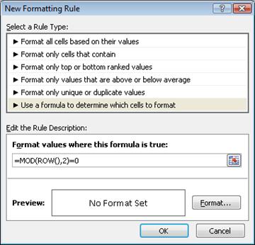
In the New Formatting Rule dialog box, under Select a Rule Type, click Use a formula to determine which cells to format.
In the Format values where this formula is true box, enter =MOD(ROW(),2)=0, as shown in the following illustration.
In the Format Cells dialog box, click the Fill tab.
Select the background or pattern color that you want to use for the shaded rows, and then click OK.
At this point, the color you just selected should appear in the Preview window in the New Formatting Rule dialog box.
To apply the formatting to the cells on your worksheet, click OK
Note: To view or edit the conditional formatting rule, on the Home tab, in the Styles group, click the arrow next to Conditional Formatting, and then click Manage Rules.
Another way to quickly add shading or banding to alternate rows is by applying a predefined Excel table style. This is useful when you want to format a specific range of cells, and you want the additional benefits that you get with a table, such the ability to quickly display total rows or header rows in which filter drop-down lists automatically appear.
By default, banding is applied to the rows in a table to make the data easier to read. The automatic banding continues if you add or delete rows in the table.
If you find you want the table style without the table functionality, you can convert the table to a regular range of data. If you do this, however, you won’t get the automatic banding as you add more data to your range.
On the worksheet, select the range of cells that you want to format.
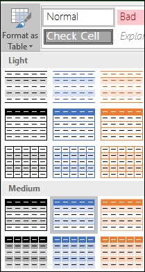
On the Home tab, in the Styles group, click Format as Table.
Under Light, Medium, or Dark, click the table style that you want to use.
Tip: Custom table styles are available under Custom after you create one or more of them. For information about how to create a custom table style, see Format an Excel table.
In the Format as Table dialog box, click OK.
Notice that the Banded Rows check box is selected by default in the Table Style Options group.
If you want to apply shading to alternate columns instead of alternate rows, you can clear this check box and select Banded Columns instead.
If you want to convert the Excel table back to a regular range of cells, click anywhere in the table to display the tools necessary for converting the table back to a range of data.
On the Design tab, in the Tools group, click Convert to Range.
Tip: You can also right-click the table, click Table, and then click Convert to Range.
Note: You cannot create custom conditional formatting rules to apply shading to alternate rows or columns in Excel for the web.
When you create a table in Excel for the web, by default, every other row in the table is shaded. The automatic banding continues if you add or delete rows in the table. However, you can apply shading to alternate columns. To do that:
Select any cell in the table.
Click the Table Design tab, and under Style Options, select the Banded Columns checkbox.
To remove shading from rows or columns, under Style Options, remove the checkbox next to Banded Rows or Banded Columns.
Need more help?
You can always ask an expert in the Excel Tech Community or get support in the Answers community.
Источник
Apply color to alternate rows or columns
Adding a color to alternate rows or columns (often called color banding) can make the data in your worksheet easier to scan. To format alternate rows or columns, you can quickly apply a preset table format. By using this method, alternate row or column shading is automatically applied when you add rows and columns.
Select the range of cells that you want to format.
Click Home > Format as Table.
Pick a table style that has alternate row shading.
To change the shading from rows to columns, select the table, click Design, and then uncheck the Banded Rows box and check the Banded Columns box.
Tip: If you want to keep a banded table style without the table functionality, you can convert the table to a data range. Color banding won’t automatically continue as you add more rows or columns but you can copy alternate color formats to new rows by using Format Painter.
Use conditional formatting to apply banded rows or columns
You can also use a conditional formatting rule to apply different formatting to specific rows or columns.
On the worksheet, do one of the following:
To apply the shading to a specific range of cells, select the cells you want to format.
To apply the shading to the whole worksheet, click the Select All button.
Click Home > Conditional Formatting > New Rule.
In the Select a Rule Type box, click Use a formula to determine which cells to format.
To apply color to alternate rows, in the Format values where this formula is true box, type the formula =MOD(ROW(),2)=0.
To apply color to alternate columns, type this formula: =MOD(COLUMN(),2)=0.
These formulas determine whether a row or column is even or odd numbered, and then applies the color accordingly.
In the Format Cells box, click Fill.
Pick a color and click OK.
You can preview your choice under Sample and click OK or pick another color.
To edit the conditional formatting rule, click one of the cells that has the rule applied, click Home > Conditional Formatting > Manage Rules > Edit Rule, and then make your changes.
To clear conditional formatting from cells, select them, click Home > Clear, and pick Clear Formats.
To copy conditional formatting to other cells, click one of the cells that has the rule applied, click Home > Format Painter  , and then click the cells you want to format.
Источник
Format an Excel table
Excel provides numerous predefined table styles that you can use to quickly format a table. If the predefined table styles don’t meet your needs, you can create and apply a custom table style. Although you can delete only custom table styles, you can remove any predefined table style so that it is no longer applied to a table.

You can further adjust the table formatting by choosing Quick Styles options for table elements, such as Header and Total Rows, First and Last Columns, Banded Rows and Columns, as well as Auto Filtering.
Note: The screen shots in this article were taken in Excel 2016. If you have a different version your view might be slightly different, but unless otherwise noted, the functionality is the same.
Choose a table style
When you have a data range that is not formatted as a table, Excel will automatically convert it to a table when you select a table style. You can also change the format for an existing table by selecting a different format.
Select any cell within the table, or range of cells you want to format as a table.
On the Home tab, click Format as Table.
Click the table style that you want to use.
Auto Preview — Excel will automatically format your data range or table with a preview of any style you select, but will only apply that style if you press Enter or click with the mouse to confirm it. You can scroll through the table formats with the mouse or your keyboard’s arrow keys.
When you use Format as Table, Excel automatically converts your data range to a table. If you don’t want to work with your data in a table, you can convert the table back to a regular range while keeping the table style formatting that you applied. For more information, see Convert an Excel table to a range of data.
Once created, custom table styles are available from the Table Styles gallery under the Custom section.
Custom table styles are only stored in the current workbook, and are not available in other workbooks.
Create a custom table style
Select any cell in the table you want to use to create a custom style.
On the Home tab, click Format as Table, or expand the Table Styles gallery from the Table Tools > Design tab (the Table tab on a Mac).
Click New Table Style, which will launch the New Table Style dialog.

In the Name box, type a name for the new table style.
In the Table Element box, do one of the following:
To format an element, click the element, then click Format, and then select the formatting options you want from the Font, Border or Fill tabs.
To remove existing formatting from an element, click the element, and then click Clear.
Under Preview, you can see how the formatting changes that you made affect the table.
To use the new table style as the default table style in the current workbook, select the Set as default table style for this document check box.
Delete a custom table style
Select any cell in the table from which you want to delete the custom table style.
On the Home tab, click Format as Table, or expand the Table Styles gallery from the Table Tools > Design tab (the Table tab on a Mac).
Under Custom, right-click the table style that you want to delete, and then click Delete on the shortcut menu.
Note: All tables in the current workbook that are using that table style will be displayed in the default table format.
Select any cell in the table from which you want to remove the current table style.
On the Home tab, click Format as Table, or expand the Table Styles gallery from the Table Tools > Design tab (the Table tab on a Mac).
The table will be displayed in the default table format.
Note: Removing a table style does not remove the table. If you don’t want to work with your data in a table, you can convert the table to a regular range. For more information, see Convert an Excel table to a range of data.
There are several table style options that can be toggled on and off. To apply any of these options:
Select any cell in the table.
Go to Table Tools > Design, or the Table tab on a Mac, and in the Table Style Options group, check or uncheck any of the following:
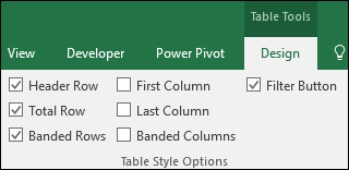
Header Row — Apply or remove formatting from the first row in the table.
Total Row — Quickly add SUBTOTAL functions like SUM, AVERAGE, COUNT, MIN/MAX to your table from a drop-down selection. SUBTOTAL functions allow you to include or ignore hidden rows in calculations.
First Column — Apply or remove formatting from the first column in the table.
Last Column — Apply or remove formatting from the last column in the table.
Banded Rows — Display odd and even rows with alternating shading for ease of reading.
Banded Columns — Display odd and even columns with alternating shading for ease of reading.
Filter Button — Toggle AutoFilter on and off.
In Excel for the web, you can apply table style options to format the table elements.
Choose table style options to format the table elements
There are several table style options that can be toggled on and off. To apply any of these options:
Select any cell in the table.
On the Table Design tab, under Style Options, check or uncheck any of the following:
Header Row — Apply or remove formatting from the first row in the table.
Total Row — Quickly add SUBTOTAL functions like SUM, AVERAGE, COUNT, MIN/MAX to your table from a drop-down selection. SUBTOTAL functions allow you to include or ignore hidden rows in calculations.
Banded Rows — Display odd and even rows with alternating shading for ease of reading.
First Column — Apply or remove formatting from the first column in the table.
Last Column — Apply or remove formatting from the last column in the table.
Banded Columns — Display odd and even columns with alternating shading for ease of reading.
Filter Button — Toggle AutoFilter on and off.
Need more help?
You can always ask an expert in the Excel Tech Community or get support in the Answers community.
Источник
Add or change the background color of a table
- Click a cell in the table.
- Under Table Tools, on the Design tab, in the Table Styles group, click the arrow next to Shading, and then point to Table Background.
- Click the color that you want, or to choose no color, click No Fill.
Contents
- 1 How do you change the table grid color in Excel?
- 2 How do you change the appearance of a table in Excel?
- 3 How do you shade cells in Excel?
- 4 How do I change the default grid color in Excel?
- 5 How do you change table shading?
- 6 How do I color a cell in a latex table?
- 7 How do I color a table cell in Sharepoint?
- 8 Can’t change Excel cell color?
- 9 How do I make an Excel sheet GREY and white?
- 10 How do I change the color of a cell in a formula?
- 11 How do you fill color in Excel without losing lines?
- 12 How do I alternate row colors in Excel without a table?
- 13 What are color grid lines?
- 14 Which option allows you to change the color of table rows columns or cells?
- 15 How can you apply a new table style to a table?
- 16 Why is my table of contents highlighted in GREY?
- 17 How do I color text in latex?
- 18 How do I color a column in latex?
- 19 How do you highlight words in latex?
- 20 Can you color code Microsoft lists?
How do you change the table grid color in Excel?
Click File > Excel > Options. In the Advanced category, under Display options for this worksheet, make sure that the Show gridlines check box is selected. In the Gridline color box, click the color you want. Tip: To return gridlines to the default color, click Automatic.
How do you change the appearance of a table in Excel?
Choose a table style
- Select any cell within the table, or range of cells you want to format as a table.
- On the Home tab, click Format as Table.
- Click the table style that you want to use.
How do you shade cells in Excel?
Click the Format menu, and then click Cells. In the Format Cells dialog box, click the Fill tab.
Apply or remove a cell shading in Excel for Mac
- In the Background color box, select a color.
- In the Pattern color box, select a color for the lines of the pattern.
- In the Pattern style box, select a pattern.
How do I change the default grid color in Excel?
You can change the color of the default gridlines in Excel from the File tab, by selecting Options, Advanced. In the Display options for this worksheet section, click the Gridline color drop-down box and select a color from the color palette, as shown below. (Make sure the Show gridlines check box is selected.)
How do you change table shading?
Add or remove shading in a table
- Select the cells you want to change.
- On the Table Tools Design tab (the Table Tools Layout tab in OneNote), click the Shading menu.
- Under Theme Colors or Standard Colors, select the shading color you want.
How do I color a cell in a latex table?
Color a cell. Use this command anywhere inside the cell. For example, if you wanted a cell with a cyan background, use cellcolor[cymk]{1,0,0,0} . If you wanted a column to be red background, use >{columncolor{red}} or >{columncolor[rgb]{1,0,0}} in your table preamble.
How do I color a table cell in Sharepoint?
After you insert your table you will need to find the Edit Source button to find the code view for the section of the page you are editing. Find the cell in your table and add the background color style to it.
Can’t change Excel cell color?
1 Answer
- Highlight the cells containing the fill color that you have previously been unable to remove.
- Click the “Conditional Formatting” drop-down menu in the “Styles” section of the ribbon.
- Click the “Clear Rules” option at the bottom of the menu, then click the “Clear Rules From Selected Cells” option.
How do I make an Excel sheet GREY and white?
Click the “Format” button. Click the “Fill” tab and select the gray color you prefer from the Background Color swatch. Click “OK” to confirm your selection.
How do I change the color of a cell in a formula?
Change the formula to use H if you want to.
- Select cell A2.
- click Conditional Formatting on the Home ribbon.
- click New Rule.
- click Use a formula to determine which cells to format.
- click into the formula box and enter the formula. =$F2
- click the Format button and select a red color.
- close all dialogs.
How do you fill color in Excel without losing lines?
Select the cells that are missing the gridlines, or hit Control + A to select the entire worksheet. Then, under the Home tab in the Font group change the color of the cells by clicking on the little arrow to the right of the can of spilling paint and choosing no fill.
How do I alternate row colors in Excel without a table?
Shade Alternate Rows
- Select a range.
- On the Home tab, in the Styles group, click Conditional Formatting.
- Click New Rule.
- Select ‘Use a formula to determine which cells to format’.
- Enter the formula =MOD(ROW(),2)
- Select a formatting style and click OK.
What are color grid lines?
Created by digital media artist and software developer Øyvind Kolås as a visual experiment, the technique, which Kolås calls the ‘colour assimilation grid illusion’, achieves its effect by simply laying a grid of selectively coloured lines over an original black-and-white image.
Which option allows you to change the color of table rows columns or cells?
Select the cells in which you want to add or change the fill color. On the Tables tab, under Table Styles, click the arrow next to Fill. On the Fill menu, click the color you want.
Remove the fill color.
| To | Do this |
|---|---|
| Use a solid color as the fill | Click the Solid tab, and then click the color that you want. |
How can you apply a new table style to a table?
Click in the table that you want to format. Under Table Tools, click the Design tab. In the Table Styles group, rest the pointer over each table style until you find a style that you want to use. Click the style to apply it to the table.
Why is my table of contents highlighted in GREY?
Answer: It is because the text is within a field.If you do not want the text to be in a field, you can unlink the field by pressing Ctrl+Shift+F9 when you have the text selected.
How do I color text in latex?
You can use the xcolor package. It provides textcolor{}{} as well as color{} to switch the color for some give text or until the end of the group/environment. You can get different shades of gray by using black!
How do I color a column in latex?
Columns can be colored using following ways:
- Defining column color property outside the table tag using newcolumntype : newcolumntype{a}{ >{columncolor{yellow}} c }
- Defining column color property inside the table parameters begin{tabular}{ | >{columncolor{red}} c | l | l }
How do you highlight words in latex?
Highlighting text
Now, text can be highlighted by simply using the command hl{text} .
Can you color code Microsoft lists?
Re: Microsoft Lists Calendar View color coding
currently color coding is not supported in modern calendar list views.

Color in Excel (Table of Contents)
- Introduction to Color in Excel
- Ways to Change Background Color
Introduction to Color in Excel
Colors are generally used to highlight a group of cells in Excel. The excel contains the index of 56 colors. By using conditional formatting, we can put some conditions and apply different colors for different conditions if we want to change the background color of the cell in Excel. We usually select the cells and click the Fill color option; then, the background color will get changed if we want to change the cell’s background colour with the cell automatically.
Ways to Change Background Color
There are two ways to change the background color.
You can download this Color Excel Template here – Color Excel Template
1. Change the color of the cell based on the current value
- Here the background color of the cell changes when the cell value in the Excel changes.
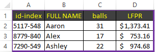
- For example, we have taken the following dataset. we want the USD Amount greater than 10,000 as blue color and remaining red color.

- Select the range of the cells which we want to change. Then go to the Home tab, go to the styles and select the conditional formatting.

- Now click on the new rules.
- A dialog appears stating the selection of the row. Select the format of the cells based on the cell value.

- Now give the range of values which are greater than 10,000 and select the color as blue color.


- Now click on the format option.
- A color box appears and makes the Pattern Color as Automatic, so Select color as blue and click on OK.

- We can observe that the sample option is blue because we have selected the blue color.

- We can observe the selected color in the format option. And click the Ok option.

- Now we can use the same procedure for selecting the color for less value. A dialog appears stating the selection of the row. Select the format of the cells based on the cell value. A dialog appears stating the selection of the row. Select the format of the cells based on the cell value. Now give the range of values which are less than 10,000 and select the color as red color.

- The color box appears and makes the pattern as automatic and Select color like blue and click OK.
- The output will be as follows.

2. Change the background color of special cells
- This is another way of color the background of the particular cell. First, go to the home tab, then select the conditional formatting.

- Select the new rules.
- The formatting dialog box appears to click on the cells which need to format, which is at the end of the dialog box.

- Click on the arrow option at the right end.
- Write the new formatting rule using the keyword Is Blank condition. This Is Blank is used to highlighting the background cells which are empty.

- Click on the Format option. And select the blue color.

- Click on the Ok button.

- The output will be as follows.

3. Sort the Excel by it Color
- Sorting is one of the methods to select a particular color. First, select the cells, right-click on them, select the sort option, and then select the highest value by color.

- Click the ok button.
- And Filter the color by its color.


- And the output will be as follows.
Change the cell color based on the current value.
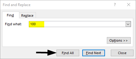
- First, go to the home tab, select the Find and select option, and select the Find option.
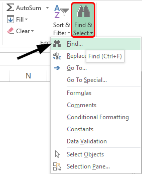
- Select the value which we want to select. Click on the Find all option.
- Click on the values range which we want the cells we want to highlight.
- Click on the Select by value option. And select the Greater in the list.
- Click on the range of the cells we want to highlight. Click on the select option.
- Now select the color as blue for the greater value.
- And the output will be as follows.
Conditional Formatting in Excel
- Conditional formatting is generally used to color data bars and icons in the cells.
- To do the conditional formatting in Excel, first, we take the required data set.
- Then go to the Home tab and select the conditional formatting option ad put the desired rule which we want to specify, and mention the color which we want to give to the cells of the particular condition.
- Then a dialog box appears on the screen then simply gives the values we want a particular condition so that the color will be applied successfully.
- Now select the formatting styles from the drop-down. Here we select the color for the condition. Then click the OK. The conditional formatting will be applied to all the cells at a time. This is one way of adding colors to the cells.
Things to Remember About Color in Excel
- The colors in excel play a major role in highlighting a particular range of cells.
- Here we generally use the two approaches like make the background color cells based on the value, and another way is to change the background of special cells.
- The excel contains the index of 56 colors. By using conditional formatting, we can put some conditions and apply different colors for different conditions.
- We can also sort the colors based on the colors.
- We can highlight the empty cells with the colors.
- Through cells, we can highlight the greater values and the lower value with different colors.
Recommended Articles
This has been a guide to Color in Excel. Here we discuss How to use Color in Excel along with practical examples and a downloadable excel template. You can also go through our other suggested articles –
- Alternate Row Color Excel
- Excel Sum by Color
- Count Colored Cells In Excel
- Excel Sort by color
Содержание
- Описание работы функции
- Пример использования
- Свойство .Interior.Color объекта Range
- Заливка ячейки цветом в VBA Excel
- Вывод сообщений о числовых значениях цветов
- Форматирование диапазона
- Нажатие кнопки Enter
- Вставка символа
- Добавление дополнительного символа
- Коды различных цветов в MS Excel 2003
Описание работы функции
Функция =ЦВЕТЗАЛИВКИ(ЯЧЕЙКА) возвращает код цвета заливки выбранной ячейки. Имеет один обязательный аргумент:
- ЯЧЕЙКА – ссылка на ячейку, для которой необходимо применить функцию.
Ниже представлен пример, демонстрирующий работу функции.

Следует обратить внимание на тот факт, что функция не пересчитывается автоматически. Это связано с тем, что изменение цвета заливки ячейки Excel не приводит к пересчету формул. Для пересчета формулы необходимо пользоваться сочетанием клавиш Ctrl+Alt+F9
Пример использования
Так как заливка ячеек значительно упрощает восприятие данных, то пользоваться ей любят практически все пользователи. Однако есть и большой минус – в стандартном функционале Excel отсутствует возможность выполнять операции на основе цвета заливки. Нельзя просуммировать ячейки определенного цвета, посчитать их количество, найти максимальное и так далее.
С помощью функции ЦВЕТЗАЛИВКИ все это становится выполнимым. Например, “протяните” данную формулу с цветом заливки в соседнем столбце и производите вычисления на основе числового кода ячейки.
Свойство .Interior.Color объекта Range
Начиная с Excel 2007 основным способом заливки диапазона или отдельной ячейки цветом (зарисовки, добавления, изменения фона) является использование свойства .Interior.Color объекта Range путем присваивания ему значения цвета в виде десятичного числа от 0 до 16777215 (всего 16777216 цветов).
Заливка ячейки цветом в VBA Excel
Пример кода 1:
|
Sub ColorTest1() Range(“A1”).Interior.Color = 31569 Range(“A4:D8”).Interior.Color = 4569325 Range(“C12:D17”).Cells(4).Interior.Color = 568569 Cells(3, 6).Interior.Color = 12659 End Sub |
Поместите пример кода в свой программный модуль и нажмите кнопку на панели инструментов «Run Sub» или на клавиатуре «F5», курсор должен быть внутри выполняемой программы. На активном листе Excel ячейки и диапазон, выбранные в коде, окрасятся в соответствующие цвета.
Есть один интересный нюанс: если присвоить свойству .Interior.Color отрицательное значение от -16777215 до -1, то цвет будет соответствовать значению, равному сумме максимального значения палитры (16777215) и присвоенного отрицательного значения. Например, заливка всех трех ячеек после выполнения следующего кода будет одинакова:
|
Sub ColorTest11() Cells(1, 1).Interior.Color = –12207890 Cells(2, 1).Interior.Color = 16777215 + (–12207890) Cells(3, 1).Interior.Color = 4569325 End Sub |
Вывод сообщений о числовых значениях цветов
Числовые значения цветов запомнить невозможно, поэтому часто возникает вопрос о том, как узнать числовое значение фона ячейки. Следующий код VBA Excel выводит сообщения о числовых значениях присвоенных ранее цветов.
Пример кода 2:
|
Sub ColorTest2() MsgBox Range(“A1”).Interior.Color MsgBox Range(“A4:D8”).Interior.Color MsgBox Range(“C12:D17”).Cells(4).Interior.Color MsgBox Cells(3, 6).Interior.Color End Sub |
Вместо вывода сообщений можно присвоить числовые значения цветов переменным, объявив их как Long.
Форматирование диапазона
Самый известный способ поставить прочерк в ячейке – это присвоить ей текстовый формат. Правда, этот вариант не всегда помогает.
- Выделяем ячейку, в которую нужно поставить прочерк. Кликаем по ней правой кнопкой мыши. В появившемся контекстном меню выбираем пункт «Формат ячейки». Можно вместо этих действий нажать на клавиатуре сочетание клавиш Ctrl+1.
- Запускается окно форматирования. Переходим во вкладку «Число», если оно было открыто в другой вкладке. В блоке параметров «Числовые форматы» выделяем пункт «Текстовый». Жмем на кнопку «OK».

После этого выделенной ячейке будет присвоено свойство текстового формата. Все введенные в нее значения будут восприниматься не как объекты для вычислений, а как простой текст. Теперь в данную область можно вводить символ «-» с клавиатуры и он отобразится именно как прочерк, а не будет восприниматься программой, как знак «минус».

Существует ещё один вариант переформатирования ячейки в текстовый вид. Для этого, находясь во вкладке «Главная», нужно кликнуть по выпадающему списку форматов данных, который расположен на ленте в блоке инструментов «Число». Открывается перечень доступных видов форматирования. В этом списке нужно просто выбрать пункт «Текстовый».

Нажатие кнопки Enter
Но данный способ не во всех случаях работает. Зачастую, даже после проведения этой процедуры при вводе символа «-» вместо нужного пользователю знака появляются все те же ссылки на другие диапазоны. Кроме того, это не всегда удобно, особенно если в таблице ячейки с прочерками чередуются с ячейками, заполненными данными. Во-первых, в этом случае вам придется форматировать каждую из них в отдельности, во-вторых, у ячеек данной таблицы будет разный формат, что тоже не всегда приемлемо. Но можно сделать и по-другому.
- Выделяем ячейку, в которую нужно поставить прочерк. Жмем на кнопку «Выровнять по центру», которая находится на ленте во вкладке «Главная» в группе инструментов «Выравнивание». А также кликаем по кнопке «Выровнять по середине», находящейся в том же блоке. Это нужно для того, чтобы прочерк располагался именно по центру ячейки, как и должно быть, а не слева.
- Набираем в ячейке с клавиатуры символ «-». После этого не делаем никаких движений мышкой, а сразу жмем на кнопку Enter, чтобы перейти на следующую строку. Если вместо этого пользователь кликнет мышкой, то в ячейке, где должен стоять прочерк, опять появится формула.
Данный метод хорош своей простотой и тем, что работает при любом виде форматирования. Но, в то же время, используя его, нужно с осторожностью относиться к редактированию содержимого ячейки, так как из-за одного неправильного действия вместо прочерка может опять отобразиться формула.
Вставка символа
Ещё один вариант написания прочерка в Эксель – это вставка символа.
- Выделяем ячейку, куда нужно вставить прочерк. Переходим во вкладку «Вставка». На ленте в блоке инструментов «Символы» кликаем по кнопке «Символ».
- Находясь во вкладке «Символы», устанавливаем в окне поля «Набор» параметр «Символы рамок». В центральной части окна ищем знак «─» и выделяем его. Затем жмем на кнопку «Вставить».

После этого прочерк отразится в выделенной ячейке.

Существует и другой вариант действий в рамках данного способа. Находясь в окне «Символ», переходим во вкладку «Специальные знаки». В открывшемся списке выделяем пункт «Длинное тире». Жмем на кнопку «Вставить». Результат будет тот же, что и в предыдущем варианте.

Данный способ хорош тем, что не нужно будет опасаться сделанного неправильного движения мышкой. Символ все равно не изменится на формулу. Кроме того, визуально прочерк поставленный данным способом выглядит лучше, чем короткий символ, набранный с клавиатуры. Главный недостаток данного варианта – это потребность выполнить сразу несколько манипуляций, что влечет за собой временные потери.
Добавление дополнительного символа
Кроме того, существует ещё один способ поставить прочерк. Правда, визуально этот вариант не для всех пользователей будет приемлемым, так как предполагает наличие в ячейке, кроме собственно знака «-», ещё одного символа.
- Выделяем ячейку, в которой нужно установить прочерк, и ставим в ней с клавиатуры символ «‘». Он располагается на той же кнопке, что и буква «Э» в кириллической раскладке. Затем тут же без пробела устанавливаем символ «-».
- Жмем на кнопку Enter или выделяем курсором с помощью мыши любую другую ячейку. При использовании данного способа это не принципиально важно. Как видим, после этих действий на листе был установлен знак прочерка, а дополнительный символ «’» заметен лишь в строке формул при выделении ячейки.

Существует целый ряд способов установить в ячейку прочерк, выбор между которыми пользователь может сделать согласно целям использования конкретного документа. Большинство людей при первой неудачной попытке поставить нужный символ пытаются сменить формат ячеек. К сожалению, это далеко не всегда срабатывает. К счастью, существуют и другие варианты выполнения данной задачи: переход на другую строку с помощью кнопки Enter, использование символов через кнопку на ленте, применение дополнительного знака «’». Каждый из этих способов имеет свои достоинства и недостатки, которые были описаны выше. Универсального варианта, который бы максимально подходил для установки прочерка в Экселе во всех возможных ситуациях, не существует.
Коды различных цветов в MS Excel 2003
Коды различных цветов при использовании конструкции типа .Interior.ColorIndex. Бесцветный код: -4142

Источники
- https://micro-solution.ru/projects/addin_vba-excel/color_interior
- https://vremya-ne-zhdet.ru/vba-excel/tsvet-yacheyki-zalivka-fon/
- http://word-office.ru/kak-sdelat-chtoby-vmesto-nulya-byl-procherk-v-excel.html
- http://aqqew.blogspot.com/2011/03/ms-excel-2003.html
How to Add Alternate Row Color in Excel?
Below mentioned are the two different methods to add color to alternative rows:
- Add alternative row colors using Excel table styles
- Highlight alternative rows using Excel “Conditional Formatting” option
Now, let us discuss each method in detail with an example.
Table of contents
- How to Add Alternate Row Color in Excel?
- #1 Add Alternative Row Color Using Excel Table Styles
- #2 Highlight Alternate Row Color using Excel Conditional Formatting
- Benefits of using Excel Alternate Row Colors
- Things to Remember
- Recommended Articles
#1 Add Alternative Row Color Using Excel Table Styles
The quickest and most straightforward approach to apply row shading in Excel is by utilizing predefined.
- First, we must select the data or range where we want to add the color in a row.

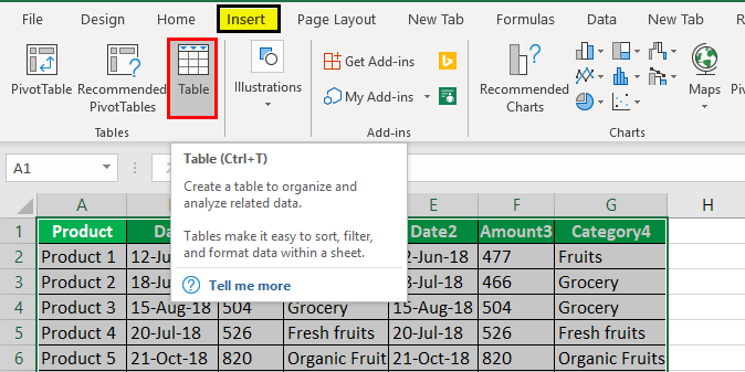
- Then, click on the “Insert” tab on the Excel ribbon and click “Table” to choose the function.

- When we click on the “Table,” the dialog box will select the range.

- Click on the “OK.” Now, we will get the table with alternate row colors in Excel, as shown below:

- Suppose we do not want the table with rows. We would preferably have alternate column shading just without the table usefulness. We can undoubtedly change over the table back to a standard range. We need to select any cell inside the table, right-click and choose “Convert to Range” from the setting menu.

- Then, select the table or data, and go to the “Design” tab.

- Next, we need to go to table style and choose the color of the table which is required and selected by us.


#2 Highlight Alternate Row Color using Excel Conditional Formatting
- Step 1: First, we need to select the data or range in the Excel sheet.
- Step 2: Go to the “Home” tab and “Styles” group, and click on conditional formatting in the ExcelConditional formatting is a technique in Excel that allows us to format cells in a worksheet based on certain conditions. It can be found in the styles section of the Home tab.read more ribbon.

- Step 3: Choose a “New Rule” from the drop-down list in excelA drop-down list in excel is a pre-defined list of inputs that allows users to select an option.read more:

- Step 4: In the “New Formatting Rule” dialog box, we must choose the option at the bottom of the dialog box, “Use a formula to determine which cells to format,” and insert the following formula in a tab to get the result
- =MOD(ROW(),2)=0

- Step 5: Click the “Format” button on the right-hand side, click on the switch to the “Fill” tab, and choose the background color we want to use or required for the banded rows in the Excel sheet.

- Step 6: In the dialog box, as shown above, the color we have selected will appear under the “Sample” at the bottom of the dialog box. If we are satisfied with the color, click “OK” to choose the same color, which shows in a sample.
- Step 7: Once we click on “OK,” it will carry us back to the “New Formatting Rule” window in the Excel sheet, and when you click “OK” again, apply the Excel color to the alternate row of the certain rows. Click “OK.” We will get the alternate row color in Excel with yellow color, as shown below.
Benefits of using Excel Alternate Row Colors
- To improve the readability of the Excel sheet, some users shade every other row in a huge Excel sheet.
- Colors can enable us to envision our information adequately by empowering us to perceive gatherings of related data by sight.
- When we use the color in your spreadsheet, this theory makes the difference.
- Adding shading to alternate rows or columns (which is called shading banding) can make the information in our worksheet less demanding to examine.
- If any rows are inserted or deleted from the row shading, it automatically adjusts to maintain our table’s pattern.
Things to Remember
- We must always use decent colors while coloring the alternate color because the bright color cannot solve our purpose.
- While using the conditional formula, we must always enter the formula in the tab. Otherwise, we will not be able to color the row.
- We should use dark colors for the text to easily read the data in the Excel worksheet.
- If we want to print your excel sheetThe print feature in excel is used to print a sheet or any data. While we can print the entire worksheet at once, we also have the option of printing only a portion of it or a specific table.read more, we must ensure that we use a light or decent color shade to highlight the rows to read it very easily.
- We must try not to use the excess conditional formatting function in our data because it creates confusion.
Recommended Articles
This article has been a guide to Excel Alternate Row Color. We discuss adding color to alternate rows using table style and conditional formatting, examples, and a downloadable Excel template. You may learn more about Excel from the following articles: –
- Excel Sum by Color
- Sort by Color in Excel
- Use Dynamic Tables in Excel
- How to use Excel Tables?
Reader Interactions