
You can use a formula in conjunction with an Event Macro. Pick a cell, say B2 and enter the formula:
=IF(A1>10,"black","green")
Then format B2 Custom ;;;
This will hide the displayed text.
Then place the following event macro in the worksheet code area:
Private Sub Worksheet_Calculate()
Application.EnableEvents = False
    With Range("B2")
        If .Value = "green" Then
            .Interior.Color = RGB(0, 255, 0)
        Else
            .Interior.Color = RGB(0, 0, 0)
        End If
    End With
Application.EnableEvents = True
End Sub
The macro will run every time the worksheet is re-calculated. It will exame the text in B2 (even though the text is not visible) and adjust the backgound color accordingly.
Because it is worksheet code, it is very easy to install and automatic to use:
- right-click the tab name near the bottom of the Excel window
- select View Code — this brings up a VBE window
- paste the stuff in and close the VBE window
If you have any concerns, first try it on a trial worksheet.
If you save the workbook, the macro will be saved with it.
If you are using a version of Excel later then 2003, you must save
the file as .xlsm rather than .xlsx
To remove the macro:
- bring up the VBE windows as above
- clear the code out
- close the VBE window
To learn more about macros in general, see:
http://www.mvps.org/dmcritchie/excel/getstarted.htm
and
http://msdn.microsoft.com/en-us/library/ee814735(v=office.14).aspx
To learn more about Event Macros (worksheet code), see:
http://www.mvps.org/dmcritchie/excel/event.htm
Macros must be enabled for this to work!
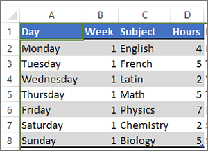
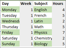
Adding a color to alternate rows or columns (often called color banding) can make the data in your worksheet easier to scan. To format alternate rows or columns, you can quickly apply a preset table format. By using this method, alternate row or column shading is automatically applied when you add rows and columns.
Here’s how:
-
Select the range of cells that you want to format.
-
Click Home > Format as Table.
-
Pick a table style that has alternate row shading.
-
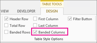
To change the shading from rows to columns, select the table, click Design, and then uncheck the Banded Rows box and check the Banded Columns box.

Tip: If you want to keep a banded table style without the table functionality, you can convert the table to a data range. Color banding won’t automatically continue as you add more rows or columns but you can copy alternate color formats to new rows by using Format Painter.
Use conditional formatting to apply banded rows or columns
You can also use a conditional formatting rule to apply different formatting to specific rows or columns.
Here’s how:
-
On the worksheet, do one of the following:
-
To apply the shading to a specific range of cells, select the cells you want to format.
-
To apply the shading to the whole worksheet, click the Select All button.
-
-
Click Home > Conditional Formatting > New Rule.
-
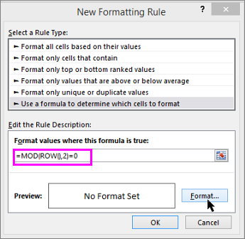
In the Select a Rule Type box, click Use a formula to determine which cells to format.
-
To apply color to alternate rows, in the Format values where this formula is true box, type the formula =MOD(ROW(),2)=0.
To apply color to alternate columns, type this formula: =MOD(COLUMN(),2)=0.
These formulas determine whether a row or column is even or odd numbered, and then applies the color accordingly.
-
Click Format.
-
In the Format Cells box, click Fill.
-
Pick a color and click OK.
-
You can preview your choice under Sample and click OK or pick another color.
Tips:
-
To edit the conditional formatting rule, click one of the cells that has the rule applied, click Home > Conditional Formatting > Manage Rules > Edit Rule, and then make your changes.
-
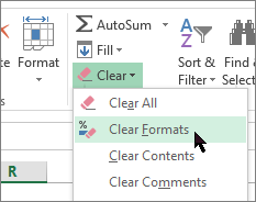
To clear conditional formatting from cells, select them, click Home > Clear, and pick Clear Formats.
-
To copy conditional formatting to other cells, click one of the cells that has the rule applied, click Home > Format Painter
, and then click the cells you want to format.
-
 , and then click the cells you want to format.
Need more help?
Want more options?
Explore subscription benefits, browse training courses, learn how to secure your device, and more.
Communities help you ask and answer questions, give feedback, and hear from experts with rich knowledge.
Based on certain values in our worksheet, we might decide to format the sheet by assigning colors based on values. In this tutorial, we will explore how to change color in excel based on values in Excel 2013, 2010 and 2016. We will also learn how to use Excel formulas to change the background colors of cells with formula errors or blank cells.
 Figure 1 – How to change cell color based on the value
How to Change Cell Color Based On Value with Conditional Formatting
When we have a table and wish to change the color of certain cells dynamically, Excel conditional formatting is a great tool we can use. It will help us highlight the values less than Y, greater than X or between X and Y. To begin:
- We will select the table or range where we want to change the background color of cells. Here we have selected the entire table.
- Now, we will go to the Home tab, select styles group and choose Conditional formatting
 Figure 2 – Formula for changing color
- We will select New Rule and in the New Formatting Rule dialog box, under the Select a Rule type box, we can select any rule. For now, we will select “Format Only Cells that contain”.
- In the lower part of the dialog box, where we have Format Only Cells with section, we will set the rule conditions. Next, we will choose to format only cells with a cell value between 90 and 140.
 Figure 3 – New formatting rule dialog box
- Now, we will click the Format button and choose the background color we want to apply
- In the Format Cells dialog box, we will switch to the fill tab and pick the color we want. Next, we click OK.
 Figure 4 – How to change font color based on the value
- We will be redirected back to the New Formatting Rule window. Here, we will preview the format changes in the Preview box. Once we are satisfied with everything, we will click OK.
 Figure 5 – How to change color
How to Change the Background Color for Special Cells (cells with formula errors or blanks)
- In the Home tab, we will go to the Styles group and click Conditional formatting
- Next, we will select New Rule. In the New Formatting Rule dialog, we will select the option Use a formula to determine which cells to format.
- Now, we will enter one of the following formulas in the format values where this formula is true field. In our example, we will select the formula for changing the color of blank cells
=IsBlank() – to change the background color of blank cells.
=IsError() – to change the background color of cells with formulas that return errors.
Where () should contain the highlighted cells.
 Figure 6 – Color cell based on the value of another cell
- Alternatively, we can click on Format only Cells that contain and select Blanks in the lower end of the dialog box.
 Figure 7 – Color cell based on the value of another cell
- We will select the Format button and choose the background color we want in the fill Tab.
 Figure 8 – How to change font color based on the value
- In the Format Cells dialog box, we will switch to the fill tab and pick the color we want. Next, we will click OK.
- We will be redirected back to the New Formatting Rule window. Here we will preview the format changes in the Preview box. Once we are satisfied with everything, we will click OK.
 Figure 9 – How to excel change cell based on the value of another cell.
Instant Connection to an Excel Expert
Most of the time, the problem you will need to solve will be more complex than a simple application of a formula or function. If you want to save hours of research and frustration, try our live Excelchat service! Our Excel Experts are available 24/7 to answer any Excel question you may have. We guarantee a connection within 30 seconds and a customized solution within 20 minutes.
How to fill color in excel cell using formula? You can do this by conditional formatting option. When you use colors in your excel worksheets you can instantly visualize the difference or comparison in value. Additionally, specification of important information gets easy. In order to specify the condition, you can use IF statement and then use conditional formatting to highlight the conditions.
If you are wondering how to fill color in excel cell using formula, here is your guide to it. So, read entire article.
Note: There is only one way to access conditional formatting as below
Use colors under certain conditions
1. Open the document having some data. Here is an example of test grades of students in terms of percentage. In this data many students passed while few failed. If we need to find fail students without wasting time, use conditional formatting.
2. Use the IF statement before applying colors. To do this, click on C3.
3. Now type equals sign and if in this cell. Then press Enter, the IF statement is activated
4. Now go to cell B3, click it and type st part of condition telling if the cell value is less than 40.
5. Now type comma, and then write Fail in inverted commas like this “Fail”
6. Again type comma, and then write Pass in inverted commas. This is the full condition which means that if the value is less than 40, type fail, otherwise pass.
7. When you press Enter key. The Pass word is shown because the student scored more than 40% grades.
8.In order to apply this function to all cells till end, click on the cell C3 again then click the right corner of the cell, drag vertically till B28.
9. Now to apply conditional formatting, click again on cell C3 and go to Conditional Formatting under Home tab. A drop down box appears.
10. Put your mouse at Highlight Cell Rules, a drop down box appears.
11. Click “Text That Contains” option in drop down menu.
12. A dialogue box opens. Now click the arrow at the right of blank field.
13. Now click C3 and press Enter. Notice the value is specified.
14. Now click on the down arrow. A drop box appears to select colors.
15. Click Light Red Fill for this example.
16. Click Ok. The text in cell C3 is filled with light red color.
17. Click on C3 cell, hover mouse at bottom right corner, click and drag. All the text containing word Pass get highlighted.
18. Now to find which student failed, repeat the whole procedure but type Fail in “Text That Contains” dialogue box and select “Green Fill With Dark Green Text” as the color.
19. Press Enter. Nothing happens to C3 as the cell has word Pass.
20. when you click and drag cursor from C3 to C28. All the cells having Fail written get highlighted in different color.
So this is whole process of how to fill color in excel cell using formula. Need to edit Word/Excel/PPT file free of charge? download WPS Office edit files like without any cost. Download now! to get enjoyable working experience.
There are two parts to this.
- You already have a sheet with formula.
- Going forward anything you type in as a formula in the same sheet.
I suggest a VBA solution as follows.
Press ALT + F11 to access the VBA editor. Insert a Module from the Insert Menu. Go to its Code Window and paste the following code into it.
Sub ColorFormula()

Dim inrange As Variant
Dim incell As Range
On Error Resume Next
Set inrange = Application.InputBox(Prompt:="Please Select a Range", Type:=8)
If inrange.Rows.Count = 0 Then
    MsgBox ("No Range Selected!")
    End
End If

For Each incell In inrange
    If incell.HasFormula = True Then
        incell.Font.Color = -4165632
    End If
Next

End Sub
Now from the Left Pane, click ThisWorkbook and select WorkBook SheetChange Event in the code window. A Placeholder for subroutine with End Sub shall be available for you to inert your code into it.
Paste the following code into it
If Target.HasFormula = True Then
    Target.Font.Color = -4165632
End If
In this example, Blue color is selected, you can change it to any other available color.
Exit the VBA Editor. Now every time you change a cell in any of the sheets of that workbook, the SheetChange event will fire and if it’s formula, it will change to Blue font.
Press ALT + F8 and run the ColorForlmula Macro and specify the cell range. The code will run thru each cell in the range and if already existing formula is found, it shall change the font to Blue.

![]()
Written by Allen Wyatt (last updated November 7, 2020)
This tip applies to Excel 97, 2000, 2002, and 2003
Cells in a worksheet can contain values or they can contain formulas. At some time, you may wish to somehow highlight all the cells in your worksheet that contain formulas by coloring those cells. There are several ways you can approach and solve this problem. If you don’t have a need to do the highlighting that often, a manual approach may be best. Follow these steps:
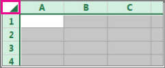
- Press either F5 or Ctrl+G. Excel displays the Go To dialog box.
- Click Special. Excel displays the Go To Special dialog box. (See Figure 1.)
- Select the Formulas radio button.
- Click OK.
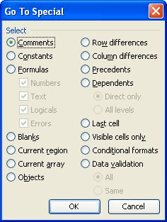
Figure 1. The Go To Special dialog box.
At this point, every cell in the worksheet that contains formulas is selected, and you can add color to those cells or format them as desired. This approach can be automated, if desired, by using a macro like the following:
Sub ColorFormulas()
    ActiveSheet.Cells.SpecialCells(xlCellTypeFormulas, 23).Select
    With Selection.Interior
        .ColorIndex = 6
        .Pattern = xlSolid
    End With
End Sub
You can run this macro as often as necessary in order to highlight the various cells that contain formulas. The only problem is that if a formula is deleted from a cell that was previously highlighted, the highlighting remains; it is not removed automatically. In this case, a different macro approach is mandated. This macro acts on a range of cells you select before running the macro.
Sub ColorFunction()
    For Each cell In Selection
        If cell.HasFormula Then
            With cell.Interior
                .ColorIndex = 6
                .Pattern = xlSolid
            End With
        Else
            cell.Interior.ColorIndex = xlNone
        End If
    Next cell
End Sub
The macro checks each cell in the range. If the cell contains a formula, then it is highlighted. If the cell does not contain a formula, then the highlight is turned off.
Another potential solution is to use a user-defined function along with the conditional formatting capabilities of Excel. Create the following function in the VBA Editor:
Function CellHasFormula(c As Range) As Boolean
    CellHasFormula = c.HasFormula
End Function
With this function in place, you can use the conditional formatting capabilities of Excel (detailed elsewhere in ExcelTips) to check what the formula returns. In other words, you would set a conditional format that checked the result of this formula:
=CellHasFormula(A1)
If the result is true (the cell contains a formula), then your conditional format is applied.
It is interesting to note that you don’t have to create a VBA macro to use the conditional formatting route, if you don’t want to. (Some people have a natural aversion to using macros.) Instead, you can follow these steps:
- Press Ctrl+F3. Excel displays the Define Name dialog box.
- In the Names field (at the top of the dialog box), enter a name such as FormulaInCell.
- In the Refers To field (at the bottom of the dialog box), enter the following:
- Click OK.
=GET.CELL(48,INDIRECT("rc",FALSE))
Now you can follow the techniques previously outlined for setting up the conditional formatting. The only difference is that the conditional format should check for the following formula, instead:
=FormulaInCell
If you would like to know how to use the macros described on this page (or on any other page on the ExcelTips sites), I’ve prepared a special page that includes helpful information. Click here to open that special page in a new browser tab.
ExcelTips is your source for cost-effective Microsoft Excel training.
This tip (2766) applies to Microsoft Excel 97, 2000, 2002, and 2003.
Author Bio
With more than 50 non-fiction books and numerous magazine articles to his credit, Allen Wyatt is an internationally recognized author. He is president of Sharon Parq Associates, a computer and publishing services company. Learn more about Allen…
MORE FROM ALLEN
Finding the Parent Folder
Do you need to figure out the name of the parent folder of whatever folder a worksheet is in? Believe it or not, this can …
Discover More
Checking for a List of Phrases in a Document
Once you start amassing quite a few documents, it is not uncommon to want to change phrases commonly used in those …
Discover More
Shortcut Key for Format Painter
The Format Painter is great for copying formatting from one cell to another. If you don’t want to grab the mouse to use …
Discover More
How to change the color of your cells in function of the value in your cells?

The secret to change the color? A logical test
To change the color with a formula, you MUST create a logical test.
A logical test returns TRUE or FALSE, or also 0 and 1. And it’s exactly what we need to create our own rule.
- The test returns TRUE, then we apply of custom format
- The test returns FALSE, the conditional formatting is not applied
For many people there is a confusion between a logical test and the IF function. The first argument of the IF function is the logical test and it’s just what we need.
Step 1: Test your rule before
I have seen a lot of mistake in my professional career when people wants to create their own rules. My advise is to test your rule in a cell.
For instance, you want to highlight all the cells with a value lower than 15.

So in column C, let’s write the test and see the result
=B2<15

Step 2: Copy your test as conditional formatting rules
- Select the cell where to apply the rule (here B2)
- Copy your formula with a basic copy-paste.
- Open the menu Home > Conditional Formatting > New Rule

- Select the rule type Use a formula to determine which cells to format
- In the text box, paste your test 😀

Step 3: Change the color
Once you have click on the button Format, you can change, the font, the background of the cell, the borders, ….
For instance here, we change only the color of the background when the test is TRUE.

Validate your rule to close the New Rule dialog box
Step 4: Apply the rule to many cells
At this step, the rule applies only for the cell B2. But now, we need to apply the same formula for the range B2:B9
- Open the menu Conditional Formatting > Manage Rules

- When the dialog box opens, you can see that the rule only applies on B2.

- Update this field to write the range of cells to apply the rule

- Now, all the cells where the rule is TRUE are red 😀👍😍
Other examples
Create your own rules to change the color is a very common task in Excel. Here is a list of other articles where we use the same technique.
- Compare 2 columns
- Highlight birthday
- Highlight week-end
- ….
Why it doesn’t work in my workbook 😱😱
One thing is very, very, VERY important is to selected the cell when you create your rule ❗❗❗

If you haven’t selected the correct cells when you have written or pasted your test, the rule applies in the wrong cell.
For instance, here, we have selected the cell B4 when we have pasted the test.

This is the only reason why you can have an issue between the result expected and the result you want 😉👍
Tutorial video
In this video, you will see 3 examples with 3 differente techniques
Let’s say that one of our tasks is to entering of the information about: did the ordering to a customer in the current month. Then on the basis of the information you need to select the cell in color according to the condition: which from customers have not made any orders for the past 3 months. For these customers you will need to re-send the offer.
Of course it’s the task for Excel. The program should automatically find such counterparties and, accordingly, to color ones. For these conditions we will use to the conditional formatting.
The filling cells with dates automatically
At first, you need to prepare to the structure for filling the register. First of all, let’s consider to the ready example of the automated register, which is depicted in the picture below. Today date 07.07.2018:
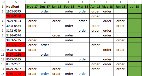
The user to need only to specify, if the customer have made an order in the current month, in the corresponding cell you should enter the text value of «order». The main condition for the allocation: if for 3 months the contractor did not make any order, his number is automatically highlighted in red.
Presented this decision should automate some work processes and to simplify to the visual data analysis.
The automatic filling of the cells with the relevant dates
At first, for the register with numbers of customers we will create to the column headers with green and up to date for months that will automatically display to the periods of time. To do this, in the cell B1 you need to enter the following formula:
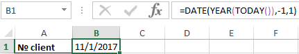
How does the formula work for automatically generating of the outgoing months?
In the picture, the formula returns the period of time passing since the date of writing this article: 17.09.2017. In the first argument in the function DATE is the nested formula that always returns the current year to today’s date thanks to the functions: YEAR and TODAY. In the second argument is the month number (-1). The negative number means that we are interested in what it was a month last time. The example of the conditions for the second argument with the value:
- 1 means the first month (January) in the year that is specified in the first argument;
- 0 – it is 1 month ago;
- -1 – there is 2 months ago from the beginning of the current year (i.e. 01.10.2016).
The last argument-is the day number of the month, which is specified in the second argument. As a result, the DATE function collects all parameters into a single value and the formula returns to the corresponding date.
Next, go to the cell C1 and type the following formula:
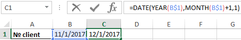
As you can see now the DATE function uses the value from the cell B1 and increases to the month number by 1 in relation to the previous cell. As the result is the 1 – the number of the following month.
Now you need to copy this formula from the cell C1 in the rest of the column headings in the range D1:AY1.
To highlight to the cell range B1:AY1 and select to the tool: «HOME»-«Cells»-«Format Cells» or just to press CTRL+1. In the dialog box that appears, in the tab «Number» in the section «Category» you need to select the option «Custom». In the «Type:» to enter the value: MMM. YY (required the letters in upper register). Because of this, we will get to the cropped display of the date values in the headers of the register, what simplifies to the visual analysis and make it more comfortable due to better readability.
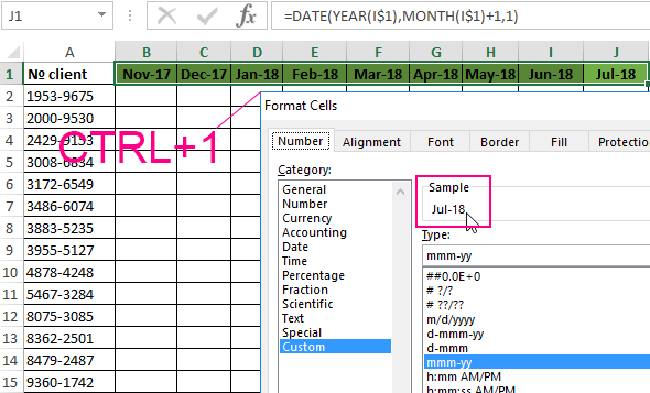
Please note! At the onset of the month of January (D1), the formula automatically changes in the date to the year in the next one.
How to select the column by color in Excel under the terms
Now you need to highlight to the cell by color which respect of the current month. Because of this, we can easily find the column in which you need to enter the actual data for this month. To do this:
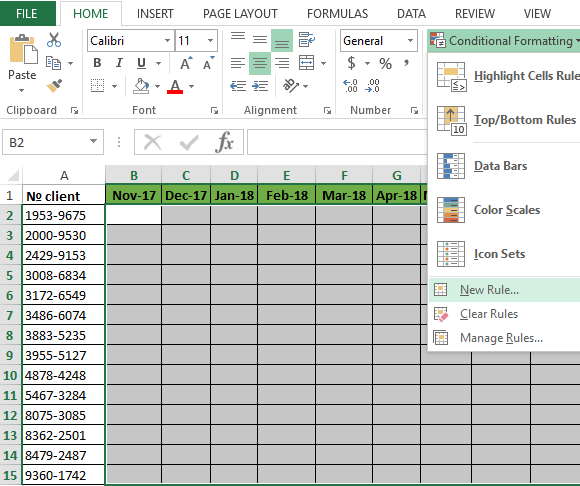
- To select the range of the cells B2:AY15 and select the tool: «HOME» -«Styles» -«Conditional Formatting»-«New Rule». And in the appeared window «New Formatting Rule» you need to select the option: «Use a formula to determine which cells to format»
- In the input field to enter the formula:
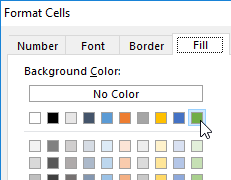
- Click «Format» and indicate on the tab «Fill» in what color (for example green) will be the selected cells of the current month. Then on all Windows for confirmation to click «OK».
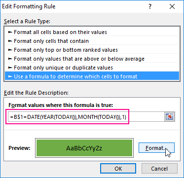
The column under the appropriate heading of the register is automatically highlighted in green accordingly to our terms and conditions:
How does the formula highlight of the column color on a condition work?
Due to the fact that before the creation of the conditional formatting rule we have covered all the table data for inputting data of register, the formatting will be active for each cell in the range B2:AY15. The mixed reference in the formula B$1 (absolute address only for rows, but for columns it is relative) determines that the formula will always to refer to the first row of each column.
Automatic highlighting of the column in the condition of the current month
The main condition for the fill by color of the cells: if the range B1:AY1 is the same date that the first day of the current month, then the cells in a column change its colors by specified in conditional formatting.
Please note! In this formula, for the last argument of the function DATE is shown 1, in the same way as for formulas in determining the dates for the column headings of the register.
In our case, is the green filling of the cells. If we open our register in next month, that it has the corresponding column is highlighted in green regardless of the current day.
The table is formatted, now we are filling it with the text value of the «order» in a mixed order of clients for current and past months.
How to highlight the cells in red color according to the condition
Now we need to highlight in red to the cells with the numbers of clients who for 3 months have not made any order. To do this:
- Select the range of the cells A2:A15 (that is, the list of the customer numbers) and select to the tool: «HOME»-«Styles»-«Conditional formatting»-«Create rule». And in the window that appeared «Create a formatting rule» to select the option: «Use the formula for determining which cells to format».
- This time in the input box to enter the formula:
- To click «Format» and specify the red color on the tab «Fill». Then on all Windows click «OK».
- Fill the cells with the text value of «order» as in the picture and look at the result:
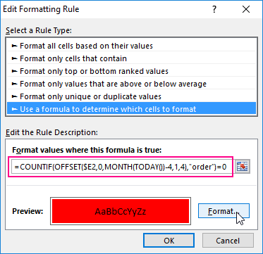
The numbers of customers are highlighted in red, if in the row has no have the value «order» in the last three cells for the current month (inclusively).
The analysis of the formula for the highlighting of cells according to the condition
Firstly, we will do by the middle part of our formula. The SHIFT function returns a range reference shifted relative to the basic range of the certain number of rows and columns. The returned reference can be a single cell or a range of cells. Optionally, you can define to the number of returned rows and columns. In our example, the function returns the reference to the cell range for the last 3 months.
The important part for our terms of highlighting in color – is belong to the first argument of the SHIFT function. It determines from which month to start the offset. In this example, there is the cell D2, that is, the beginning of the year – January. Of course for the rest of the cells in the column the row number for the base of the cell will correspond to the line number in what it is located. The following 2 arguments of the SHIFT function to determine how many rows and columns should be done offset. Since the calculations for each customer will carry in the same line, the offset value for the rows we specified is -0.
At the same time for the calculating the value of the third argument (the offset by the columns) we use to the nested formula MONTH(TODAY()), which in accordance with the terms returns to the number of the current month in the current year. From the calculated formula of the month as a number subtract the number 4, that is, in cases November we get the offset by 8 columns. And, for example, for June – there are on 2 columns only.
The last two arguments for the SHIFT function, determine the height (in the number of rows) and width (in the number of columns) of the returned range. In our example, there is the area of the cell with height on 1 row and with width on 4 columns. This range covers to the columns of 3 previous months and the current month.
The first function in the COUNTIF formula checks the condition: how many times in the returned range using the SHIFT function, we can found to the text value «order». If the function returns the value of 0, it means from the client with this number for 3 months there was not any order. And in accordance with our terms and conditions, the cell with number of this client is shown in red fill color.
If we want to register to data for customers, Excel is ideally suited for this purpose. You can easily record in the appropriate categories to the number of ordered goods, as well as the date of implementation of transaction. The problem gradually starts with arising of the data growth.
Download example automatic highlight cells by color.
If so many of them that we need to spend a few minutes looking for a specific position of the register and analysis of the information entered. In this case, it is necessary to add in the table to the register of mechanisms to automate some workflows of the user. And so we did.