
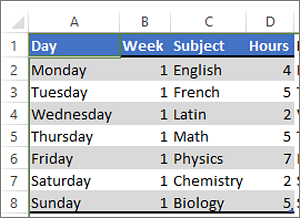
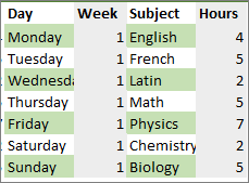
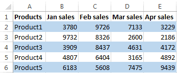
Adding a color to alternate rows or columns (often called color banding) can make the data in your worksheet easier to scan. To format alternate rows or columns, you can quickly apply a preset table format. By using this method, alternate row or column shading is automatically applied when you add rows and columns.
Here’s how:
-
Select the range of cells that you want to format.
-
Click Home > Format as Table.
-
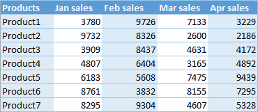
Pick a table style that has alternate row shading.
-
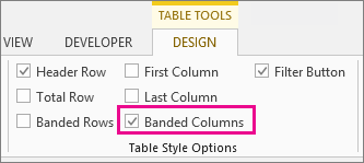
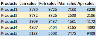
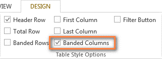
To change the shading from rows to columns, select the table, click Design, and then uncheck the Banded Rows box and check the Banded Columns box.

Tip: If you want to keep a banded table style without the table functionality, you can convert the table to a data range. Color banding won’t automatically continue as you add more rows or columns but you can copy alternate color formats to new rows by using Format Painter.
Use conditional formatting to apply banded rows or columns
You can also use a conditional formatting rule to apply different formatting to specific rows or columns.
Here’s how:
-
On the worksheet, do one of the following:
-
To apply the shading to a specific range of cells, select the cells you want to format.
-
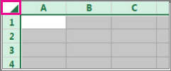
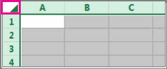
To apply the shading to the whole worksheet, click the Select All button.
-
-
Click Home > Conditional Formatting > New Rule.
-
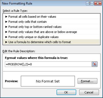
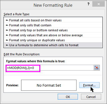
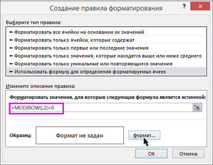
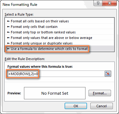
In the Select a Rule Type box, click Use a formula to determine which cells to format.
-
To apply color to alternate rows, in the Format values where this formula is true box, type the formula =MOD(ROW(),2)=0.
To apply color to alternate columns, type this formula: =MOD(COLUMN(),2)=0.
These formulas determine whether a row or column is even or odd numbered, and then applies the color accordingly.
-
Click Format.
-
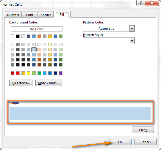
In the Format Cells box, click Fill.
-
Pick a color and click OK.
-
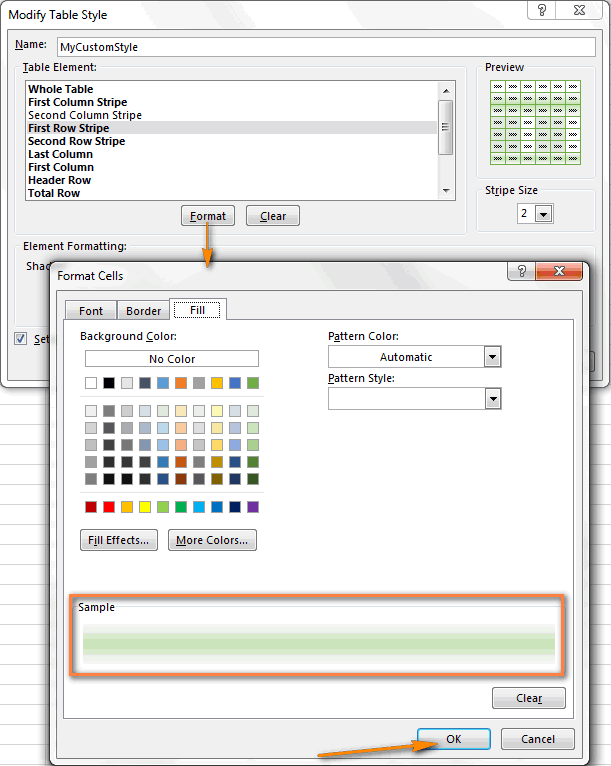
You can preview your choice under Sample and click OK or pick another color.
Tips:
-
To edit the conditional formatting rule, click one of the cells that has the rule applied, click Home > Conditional Formatting > Manage Rules > Edit Rule, and then make your changes.
-
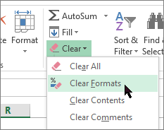
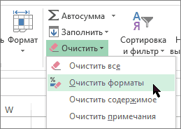
To clear conditional formatting from cells, select them, click Home > Clear, and pick Clear Formats.
-
To copy conditional formatting to other cells, click one of the cells that has the rule applied, click Home > Format Painter
, and then click the cells you want to format.
-
Need more help?
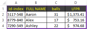
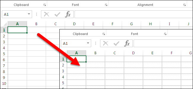
In this lesson we will learn how to change the color of a table in Excel. For this, we will initialize the original table from the previous lesson by formatting the background and cell borders.
Immediately go over to practice. We select the whole table A1:D4.
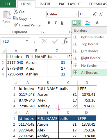
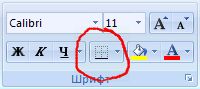
On the «Home» tab, click on the «Borders» tool, which is located in the «Font» section. From the drop-down list, select the option «All borders».
Now again in the same list, select the option «Thick outer border». Next, select the range A1:D1. In the same section of the tools, click on «Fill color» and point to «Dark Blue». Next, in the «Text color» tool, point «White».
The example of changing the color of tables
The pictures show the process of changing the boundaries in practice:
You can also change the color of a table in Excel using the more functional tool.
Select again the entire table A1:D4. Press the hotkey combination CTRL + 1 or CTRL + SHIFT + F. The multifunction dialog box «Format Cells» will appear.
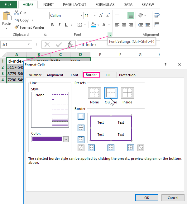
First go to the «Border» tab. In the «Presets» toolbar of this tab, click the «Inside» button. Now in the line type section, select the thickest line (second from the bottom in the right column). If necessary, set the color for the borders of the table below. Then go back to the «All» section and click on the «Outline» button. To confirm the border formatting settings, click OK.
Also we can make a colors text. Select the headings of the original table A1:D1. Open the «Format Cells» window. At present go to the «Font» tab and in the text color field select «Yellow». To change the color of the selected cell in Excel, click the «Fill» tab and click on «Black». To confirm the change of the format of the cells, click OK. Pasting cells in Excel allows you to select a row or column by color.
As you can see in the «Format Cells» window there are multiplicity of tools, that expand the possibilities of formatting data.
The helpful advice! Format the data in the last place: so you will save your working time.
The formatting opens up wide possibilities for data exposure. There are the changing fonts and sizes of text, setting background colors and patterns, paint border colors and select the type of their lines, etc. But if you slightly overdo with the color change a little, the Excel sheet becomes colorful and unreadable.
Содержание
- Change the color of the table in Excel
- The example of changing the color of tables
- Apply shading to alternate rows or columns in a worksheet
- Need more help?
- Apply color to alternate rows or columns
- Use conditional formatting to apply banded rows or columns
- Format an Excel table
- Choose a table style
- Choose table style options to format the table elements
- Need more help?
Change the color of the table in Excel
In this lesson we will learn how to change the color of a table in Excel. For this, we will initialize the original table from the previous lesson by formatting the background and cell borders.
Immediately go over to practice. We select the whole table A1:D4.
On the «Home» tab, click on the «Borders» tool, which is located in the «Font» section. From the drop-down list, select the option «All borders».
Now again in the same list, select the option «Thick outer border». Next, select the range A1:D1. In the same section of the tools, click on «Fill color» and point to «Dark Blue». Next, in the «Text color» tool, point «White».
The example of changing the color of tables
The pictures show the process of changing the boundaries in practice:
You can also change the color of a table in Excel using the more functional tool.
Select again the entire table A1:D4. Press the hotkey combination CTRL + 1 or CTRL + SHIFT + F. The multifunction dialog box «Format Cells» will appear.
First go to the «Border» tab. In the «Presets» toolbar of this tab, click the «Inside» button. Now in the line type section, select the thickest line (second from the bottom in the right column). If necessary, set the color for the borders of the table below. Then go back to the «All» section and click on the «Outline» button. To confirm the border formatting settings, click OK.
Also we can make a colors text. Select the headings of the original table A1:D1. Open the «Format Cells» window. At present go to the «Font» tab and in the text color field select «Yellow». To change the color of the selected cell in Excel, click the «Fill» tab and click on «Black». To confirm the change of the format of the cells, click OK. Pasting cells in Excel allows you to select a row or column by color.
As you can see in the «Format Cells» window there are multiplicity of tools, that expand the possibilities of formatting data.
The helpful advice! Format the data in the last place: so you will save your working time.
The formatting opens up wide possibilities for data exposure. There are the changing fonts and sizes of text, setting background colors and patterns, paint border colors and select the type of their lines, etc. But if you slightly overdo with the color change a little, the Excel sheet becomes colorful and unreadable.
Источник
Apply shading to alternate rows or columns in a worksheet
This article shows you how to automatically apply shading to every other row or column in a worksheet.
There are two ways to apply shading to alternate rows or columns —you can apply the shading by using a simple conditional formatting formula, or, you can apply a predefined Excel table style to your data.
One way to apply shading to alternate rows or columns in your worksheet is by creating a conditional formatting rule. This rule uses a formula to determine whether a row is even or odd numbered, and then applies the shading accordingly. The formula is shown here:
Note: If you want to apply shading to alternate columns instead of alternate rows, enter =MOD(COLUMN(),2)=0 instead.
On the worksheet, do one of the following:
To apply the shading to a specific range of cells, select the cells you want to format.
To apply the shading to the entire worksheet, click the Select All button.

On the Home tab, in the Styles group, click the arrow next to Conditional Formatting, and then click New Rule.
In the New Formatting Rule dialog box, under Select a Rule Type, click Use a formula to determine which cells to format.
In the Format values where this formula is true box, enter =MOD(ROW(),2)=0, as shown in the following illustration.
In the Format Cells dialog box, click the Fill tab.
Select the background or pattern color that you want to use for the shaded rows, and then click OK.
At this point, the color you just selected should appear in the Preview window in the New Formatting Rule dialog box.
To apply the formatting to the cells on your worksheet, click OK
Note: To view or edit the conditional formatting rule, on the Home tab, in the Styles group, click the arrow next to Conditional Formatting, and then click Manage Rules.
Another way to quickly add shading or banding to alternate rows is by applying a predefined Excel table style. This is useful when you want to format a specific range of cells, and you want the additional benefits that you get with a table, such the ability to quickly display total rows or header rows in which filter drop-down lists automatically appear.
By default, banding is applied to the rows in a table to make the data easier to read. The automatic banding continues if you add or delete rows in the table.
If you find you want the table style without the table functionality, you can convert the table to a regular range of data. If you do this, however, you won’t get the automatic banding as you add more data to your range.
On the worksheet, select the range of cells that you want to format.
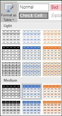
On the Home tab, in the Styles group, click Format as Table.
Under Light, Medium, or Dark, click the table style that you want to use.
Tip: Custom table styles are available under Custom after you create one or more of them. For information about how to create a custom table style, see Format an Excel table.
In the Format as Table dialog box, click OK.
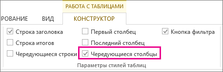
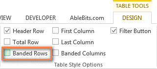
Notice that the Banded Rows check box is selected by default in the Table Style Options group.
If you want to apply shading to alternate columns instead of alternate rows, you can clear this check box and select Banded Columns instead.
If you want to convert the Excel table back to a regular range of cells, click anywhere in the table to display the tools necessary for converting the table back to a range of data.
On the Design tab, in the Tools group, click Convert to Range.
Tip: You can also right-click the table, click Table, and then click Convert to Range.
Note: You cannot create custom conditional formatting rules to apply shading to alternate rows or columns in Excel for the web.
When you create a table in Excel for the web, by default, every other row in the table is shaded. The automatic banding continues if you add or delete rows in the table. However, you can apply shading to alternate columns. To do that:
Select any cell in the table.
Click the Table Design tab, and under Style Options, select the Banded Columns checkbox.
To remove shading from rows or columns, under Style Options, remove the checkbox next to Banded Rows or Banded Columns.
Need more help?
You can always ask an expert in the Excel Tech Community or get support in the Answers community.
Источник
Apply color to alternate rows or columns
Adding a color to alternate rows or columns (often called color banding) can make the data in your worksheet easier to scan. To format alternate rows or columns, you can quickly apply a preset table format. By using this method, alternate row or column shading is automatically applied when you add rows and columns.
Select the range of cells that you want to format.
Click Home > Format as Table.
Pick a table style that has alternate row shading.
To change the shading from rows to columns, select the table, click Design, and then uncheck the Banded Rows box and check the Banded Columns box.
Tip: If you want to keep a banded table style without the table functionality, you can convert the table to a data range. Color banding won’t automatically continue as you add more rows or columns but you can copy alternate color formats to new rows by using Format Painter.
Use conditional formatting to apply banded rows or columns
You can also use a conditional formatting rule to apply different formatting to specific rows or columns.
On the worksheet, do one of the following:
To apply the shading to a specific range of cells, select the cells you want to format.
To apply the shading to the whole worksheet, click the Select All button.
Click Home > Conditional Formatting > New Rule.
In the Select a Rule Type box, click Use a formula to determine which cells to format.
To apply color to alternate rows, in the Format values where this formula is true box, type the formula =MOD(ROW(),2)=0.
To apply color to alternate columns, type this formula: =MOD(COLUMN(),2)=0.
These formulas determine whether a row or column is even or odd numbered, and then applies the color accordingly.
In the Format Cells box, click Fill.
Pick a color and click OK.
You can preview your choice under Sample and click OK or pick another color.
To edit the conditional formatting rule, click one of the cells that has the rule applied, click Home > Conditional Formatting > Manage Rules > Edit Rule, and then make your changes.
To clear conditional formatting from cells, select them, click Home > Clear, and pick Clear Formats.
To copy conditional formatting to other cells, click one of the cells that has the rule applied, click Home > Format Painter  , and then click the cells you want to format.
Источник
Format an Excel table
Excel provides numerous predefined table styles that you can use to quickly format a table. If the predefined table styles don’t meet your needs, you can create and apply a custom table style. Although you can delete only custom table styles, you can remove any predefined table style so that it is no longer applied to a table.

You can further adjust the table formatting by choosing Quick Styles options for table elements, such as Header and Total Rows, First and Last Columns, Banded Rows and Columns, as well as Auto Filtering.
Note: The screen shots in this article were taken in Excel 2016. If you have a different version your view might be slightly different, but unless otherwise noted, the functionality is the same.
Choose a table style
When you have a data range that is not formatted as a table, Excel will automatically convert it to a table when you select a table style. You can also change the format for an existing table by selecting a different format.
Select any cell within the table, or range of cells you want to format as a table.
On the Home tab, click Format as Table.
Click the table style that you want to use.
Auto Preview — Excel will automatically format your data range or table with a preview of any style you select, but will only apply that style if you press Enter or click with the mouse to confirm it. You can scroll through the table formats with the mouse or your keyboard’s arrow keys.
When you use Format as Table, Excel automatically converts your data range to a table. If you don’t want to work with your data in a table, you can convert the table back to a regular range while keeping the table style formatting that you applied. For more information, see Convert an Excel table to a range of data.
Once created, custom table styles are available from the Table Styles gallery under the Custom section.
Custom table styles are only stored in the current workbook, and are not available in other workbooks.
Create a custom table style
Select any cell in the table you want to use to create a custom style.
On the Home tab, click Format as Table, or expand the Table Styles gallery from the Table Tools > Design tab (the Table tab on a Mac).
Click New Table Style, which will launch the New Table Style dialog.

In the Name box, type a name for the new table style.
In the Table Element box, do one of the following:
To format an element, click the element, then click Format, and then select the formatting options you want from the Font, Border or Fill tabs.
To remove existing formatting from an element, click the element, and then click Clear.
Under Preview, you can see how the formatting changes that you made affect the table.
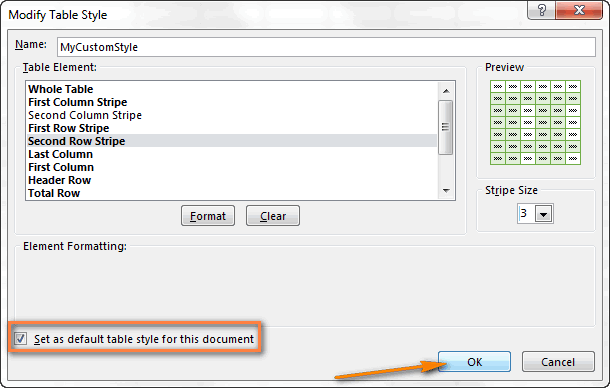
To use the new table style as the default table style in the current workbook, select the Set as default table style for this document check box.
Delete a custom table style
Select any cell in the table from which you want to delete the custom table style.
On the Home tab, click Format as Table, or expand the Table Styles gallery from the Table Tools > Design tab (the Table tab on a Mac).
Under Custom, right-click the table style that you want to delete, and then click Delete on the shortcut menu.
Note: All tables in the current workbook that are using that table style will be displayed in the default table format.
Select any cell in the table from which you want to remove the current table style.
On the Home tab, click Format as Table, or expand the Table Styles gallery from the Table Tools > Design tab (the Table tab on a Mac).
The table will be displayed in the default table format.
Note: Removing a table style does not remove the table. If you don’t want to work with your data in a table, you can convert the table to a regular range. For more information, see Convert an Excel table to a range of data.
There are several table style options that can be toggled on and off. To apply any of these options:
Select any cell in the table.
Go to Table Tools > Design, or the Table tab on a Mac, and in the Table Style Options group, check or uncheck any of the following:
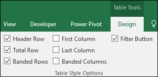
Header Row — Apply or remove formatting from the first row in the table.
Total Row — Quickly add SUBTOTAL functions like SUM, AVERAGE, COUNT, MIN/MAX to your table from a drop-down selection. SUBTOTAL functions allow you to include or ignore hidden rows in calculations.
First Column — Apply or remove formatting from the first column in the table.
Last Column — Apply or remove formatting from the last column in the table.
Banded Rows — Display odd and even rows with alternating shading for ease of reading.
Banded Columns — Display odd and even columns with alternating shading for ease of reading.
Filter Button — Toggle AutoFilter on and off.
In Excel for the web, you can apply table style options to format the table elements.
Choose table style options to format the table elements
There are several table style options that can be toggled on and off. To apply any of these options:
Select any cell in the table.
On the Table Design tab, under Style Options, check or uncheck any of the following:
Header Row — Apply or remove formatting from the first row in the table.
Total Row — Quickly add SUBTOTAL functions like SUM, AVERAGE, COUNT, MIN/MAX to your table from a drop-down selection. SUBTOTAL functions allow you to include or ignore hidden rows in calculations.
Banded Rows — Display odd and even rows with alternating shading for ease of reading.
First Column — Apply or remove formatting from the first column in the table.
Last Column — Apply or remove formatting from the last column in the table.
Banded Columns — Display odd and even columns with alternating shading for ease of reading.
Filter Button — Toggle AutoFilter on and off.
Need more help?
You can always ask an expert in the Excel Tech Community or get support in the Answers community.
Источник
Add or change the background color of a table
- Click a cell in the table.
- Under Table Tools, on the Design tab, in the Table Styles group, click the arrow next to Shading, and then point to Table Background.
- Click the color that you want, or to choose no color, click No Fill.
Contents
- 1 How do you change the table grid color in Excel?
- 2 How do you change the appearance of a table in Excel?
- 3 How do you shade cells in Excel?
- 4 How do I change the default grid color in Excel?
- 5 How do you change table shading?
- 6 How do I color a cell in a latex table?
- 7 How do I color a table cell in Sharepoint?
- 8 Can’t change Excel cell color?
- 9 How do I make an Excel sheet GREY and white?
- 10 How do I change the color of a cell in a formula?
- 11 How do you fill color in Excel without losing lines?
- 12 How do I alternate row colors in Excel without a table?
- 13 What are color grid lines?
- 14 Which option allows you to change the color of table rows columns or cells?
- 15 How can you apply a new table style to a table?
- 16 Why is my table of contents highlighted in GREY?
- 17 How do I color text in latex?
- 18 How do I color a column in latex?
- 19 How do you highlight words in latex?
- 20 Can you color code Microsoft lists?
How do you change the table grid color in Excel?
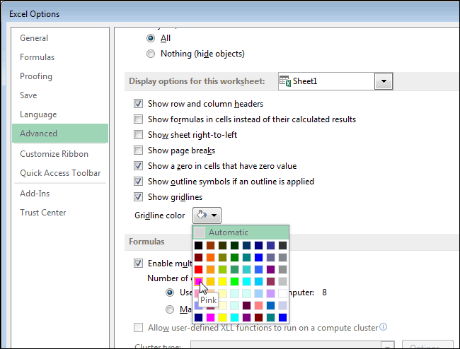
Click File > Excel > Options. In the Advanced category, under Display options for this worksheet, make sure that the Show gridlines check box is selected. In the Gridline color box, click the color you want. Tip: To return gridlines to the default color, click Automatic.
How do you change the appearance of a table in Excel?
Choose a table style
- Select any cell within the table, or range of cells you want to format as a table.
- On the Home tab, click Format as Table.
- Click the table style that you want to use.
How do you shade cells in Excel?
Click the Format menu, and then click Cells. In the Format Cells dialog box, click the Fill tab.
Apply or remove a cell shading in Excel for Mac
- In the Background color box, select a color.
- In the Pattern color box, select a color for the lines of the pattern.
- In the Pattern style box, select a pattern.
How do I change the default grid color in Excel?
You can change the color of the default gridlines in Excel from the File tab, by selecting Options, Advanced. In the Display options for this worksheet section, click the Gridline color drop-down box and select a color from the color palette, as shown below. (Make sure the Show gridlines check box is selected.)
How do you change table shading?
Add or remove shading in a table
- Select the cells you want to change.
- On the Table Tools Design tab (the Table Tools Layout tab in OneNote), click the Shading menu.
- Under Theme Colors or Standard Colors, select the shading color you want.
How do I color a cell in a latex table?
Color a cell. Use this command anywhere inside the cell. For example, if you wanted a cell with a cyan background, use cellcolor[cymk]{1,0,0,0} . If you wanted a column to be red background, use >{columncolor{red}} or >{columncolor[rgb]{1,0,0}} in your table preamble.
How do I color a table cell in Sharepoint?
After you insert your table you will need to find the Edit Source button to find the code view for the section of the page you are editing. Find the cell in your table and add the background color style to it.
Can’t change Excel cell color?
1 Answer
- Highlight the cells containing the fill color that you have previously been unable to remove.
- Click the “Conditional Formatting” drop-down menu in the “Styles” section of the ribbon.
- Click the “Clear Rules” option at the bottom of the menu, then click the “Clear Rules From Selected Cells” option.
How do I make an Excel sheet GREY and white?
Click the “Format” button. Click the “Fill” tab and select the gray color you prefer from the Background Color swatch. Click “OK” to confirm your selection.
How do I change the color of a cell in a formula?
Change the formula to use H if you want to.
- Select cell A2.
- click Conditional Formatting on the Home ribbon.
- click New Rule.
- click Use a formula to determine which cells to format.
- click into the formula box and enter the formula. =$F2
- click the Format button and select a red color.
- close all dialogs.
How do you fill color in Excel without losing lines?
Select the cells that are missing the gridlines, or hit Control + A to select the entire worksheet. Then, under the Home tab in the Font group change the color of the cells by clicking on the little arrow to the right of the can of spilling paint and choosing no fill.
How do I alternate row colors in Excel without a table?
Shade Alternate Rows
- Select a range.
- On the Home tab, in the Styles group, click Conditional Formatting.
- Click New Rule.
- Select ‘Use a formula to determine which cells to format’.
- Enter the formula =MOD(ROW(),2)
- Select a formatting style and click OK.
What are color grid lines?
Created by digital media artist and software developer Øyvind Kolås as a visual experiment, the technique, which Kolås calls the ‘colour assimilation grid illusion’, achieves its effect by simply laying a grid of selectively coloured lines over an original black-and-white image.
Which option allows you to change the color of table rows columns or cells?
Select the cells in which you want to add or change the fill color. On the Tables tab, under Table Styles, click the arrow next to Fill. On the Fill menu, click the color you want.
Remove the fill color.
| To | Do this |
|---|---|
| Use a solid color as the fill | Click the Solid tab, and then click the color that you want. |
How can you apply a new table style to a table?
Click in the table that you want to format. Under Table Tools, click the Design tab. In the Table Styles group, rest the pointer over each table style until you find a style that you want to use. Click the style to apply it to the table.
Why is my table of contents highlighted in GREY?
Answer: It is because the text is within a field.If you do not want the text to be in a field, you can unlink the field by pressing Ctrl+Shift+F9 when you have the text selected.
How do I color text in latex?
You can use the xcolor package. It provides textcolor{}{} as well as color{} to switch the color for some give text or until the end of the group/environment. You can get different shades of gray by using black!
How do I color a column in latex?
Columns can be colored using following ways:
- Defining column color property outside the table tag using newcolumntype : newcolumntype{a}{ >{columncolor{yellow}} c }
- Defining column color property inside the table parameters begin{tabular}{ | >{columncolor{red}} c | l | l }
How do you highlight words in latex?
Highlighting text
Now, text can be highlighted by simply using the command hl{text} .
Can you color code Microsoft lists?
Re: Microsoft Lists Calendar View color coding
currently color coding is not supported in modern calendar list views.
What are Excel Tables?
Tables in Excel helps group related data into one or more rows and/or columns. Once a table is created, Excel assigns a unique name to the columns and the table itself. Such names are used as structured references, which make it easy to apply Excel formulas. Therefore, tables eliminate the need to create named ranges in Excel.
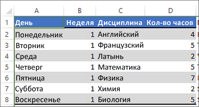
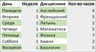
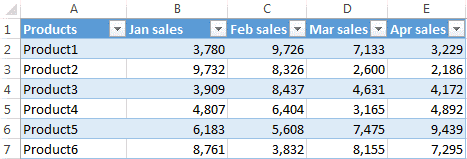
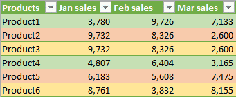
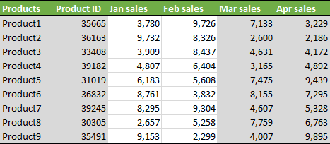
For example, the following image shows a usual data range on the left side and an Excel table on the right side. Notice the alternately colored excel rowsThe two different methods to add colour to alternative rows are adding alternative row colour using Excel table styles or highlighting alternative rows using the Excel conditional formatting option.read more and structured references (in cell J2) of the latter.
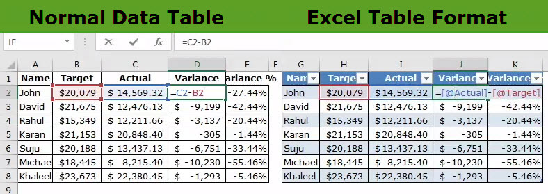
The purpose of creating tables is to make the data manageable, organized, and fit for analysis. Apart from structured references, tables offer several benefits like quick sorting and filtering, automatic expansion, easy formatting, readable formulas, and so on. Tables are extremely helpful when working with large databases.
Table of contents
- What are Excel Tables?
- How to Create Tables in Excel?
- How to Customize Tables in Excel?
- #1–Change the Name of the Table
- #2–Change the Color of the Table
- What are the Advantages of Creating Tables in Excel?
- #1–Creates Structured References Automatically
- #2–Is Dynamic in Nature
- #3–Makes it Easy to Work With PivotTables
- #4–Freezes Header Row Automatically
- #5–Helps add a Total Row Containing Functions
- #6–Eases Restoring to Usual Data Range Without Losing the Table Style
- #7–Helps add Slicers for Filtering Data
- #8–Assists in Creating Reports in Power BI
- How to Turn off Structured References in Excel?
- Frequently Asked Questions
- Recommended Articles
How to Create Tables in Excel?
You can download this Excel Tables Template here – Excel Tables Template
The steps to create a table in Excel are listed as follows:
- Ensure that the raw data does not contain any empty rows and/or columns. Further, each column should have a unique heading. If any two columns have the same headers, Excel automatically changes one of these headers once a table is created.
The raw data is shown in the following image.
Note: A column header should not contain any Excel formulas.

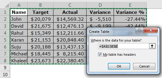
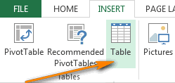
- Select any cell of the raw data and press the shortcut “Ctrl+T.” Both keys of the shortcut should be pressed together.
Note: Alternatively, after selecting a cell of the raw data, click “table” from the Insert tab of Excel. This option is in the “tables” group of the Excel ribbon.

- The “create table” dialog box opens, as shown in the following image. Excel automatically selects the range for the table. Check whether this range is correct or not. If not, it can be edited.

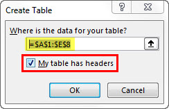
- Select or deselect the checkbox of “my table has headers.” If selected, Excel will treat the content of the first row (row 1) as column headers.
In the preceding table, row 1 does contain column headers. So, we have selected the option “my table has headers.” Next, click “Ok.”

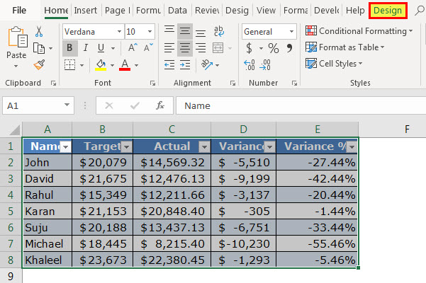
- An Excel table has been created. It is shown in the following image. Notice that the banded rows and filters (to the right of each column header) appear automatically.
Note: In Excel, banded rows are those in which color or shading is applied alternately.


How to Customize Tables in Excel?
A table can be customized by changing its name and/or the default color (or table style). Let us learn how this is done.
#1–Change the Name of the Table
When a table is created, Excel assigns a default name like “table1,” “table2,” etc., depending on whether it is the first or the second table of the current workbook.
Working with such default names may become confusing, especially when there are lots of tables. So, the solution is to assign unique names to each table.
The steps for changing the name of the Excel table are listed as follows:
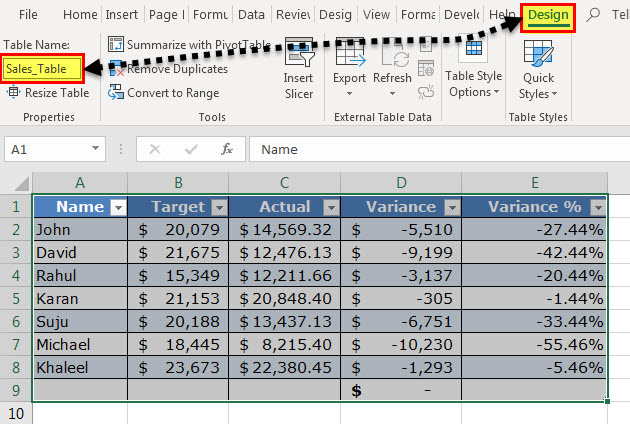
Step 1: Select the entire table. Once selected, the Design tab appears on the Excel ribbonRibbons in Excel 2016 are designed to help you easily locate the command you want to use. Ribbons are organized into logical groups called Tabs, each of which has its own set of functions.read more. This tab is shown within a red box in the following image.
Note: In place of the entire table, even if a single cell is selected, the Design tab will become visible.
Step 2: In the Design tab, perform the following tasks:
- Click inside the box under “table name.” This box is displayed in the “properties” group at the leftmost side of the ribbon.
- Enter the desired name in this box.
- Press the “Enter” key.
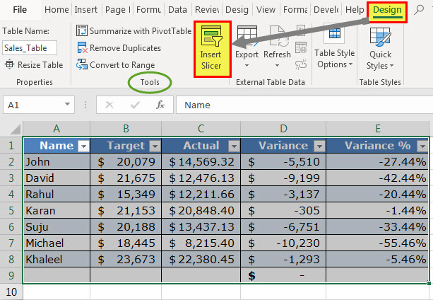
Our table has been named “Sales_Table.” This is shown in the following image.
Rules Governing the Table Names
While naming a table, the following points should be considered:
- The name should always begin with a letter, a backslash () or an underscore (_).
- The name cannot be the single letter “r” (or “R”) or “c” (or “C”).
- The name should not consist of any spaces. Instead, one can use an underscore (_) or a period (.) to separate the words.
- The name can contain numbers, but cell references should be avoided.
- The name can contain a maximum of 255 characters.
- The name of the table should be unique. In case of a duplicate name, a message will be displayed saying that a unique name should be chosen.
Note: A name is said to be duplicate if two tables within the same workbook have the same names. Further, Excel does not distinguish between the uppercase and lowercase letters in the name of a table. So, the names “abc” or “ABC” are considered the same by Excel.
#2–Change the Color of the Table
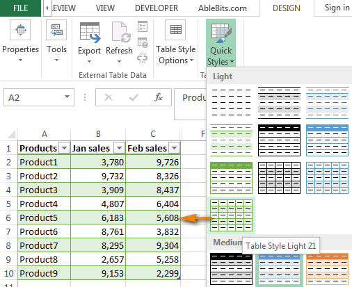
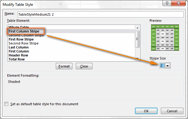
When a table is created, Excel assigns it a default color. To change the color of the table, its style needs to be changed. Excel displays a list of different table styles from which one can choose the desired option.
The steps to change the color (or style) of a table are listed as follows:
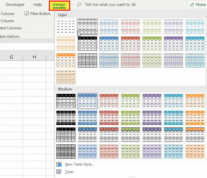
Step 1: Select either a cell of the table or the entire table. We have selected the latter. The Design tab becomes visible, as shown in the following image.

Step 2: Choose the desired color (or style) from the “table styles” group of the Design tab. To expand the list of table styles, click the “more” button displayed at the bottom right side. One can also click “new table style” to view more styles.
The following image shows the expanded list of table styles. Once the desired style is chosen, it will be applied to the entire table.
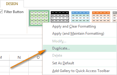
Note: The default table style of the workbook can be changed by the user. For making this change, perform the listed steps:
- Select the desired table style from the list of table styles.
- Right-click the selected table style and choose “set as default” from the context menu.
What are the Advantages of Creating Tables in Excel?
Let us discuss eight advantages of creating tables in Excel.
#1–Creates Structured References Automatically
An Excel table uses structured referencesIn Excel, structured references define data sets in columns by giving names instead of cell address. You may use the column name instead of the cell address in the formula; this makes work easier.read more for referencing one or more cells. This is in contrast with the direct cell addresses used in a normal data range. A structured reference is a combination of table and column names that are used in Excel formulasThe term «basic excel formula» refers to the general functions used in Microsoft Excel to do simple calculations such as addition, average, and comparison. SUM, COUNT, COUNTA, COUNTBLANK, AVERAGE, MIN Excel, MAX Excel, LEN Excel, TRIM Excel, IF Excel are the top ten excel formulas and functions.read more.
The major benefits of using structured references are listed as follows:
- They automatically update when new entries are added or deleted from the table.
- They are automatically created when one or more cells of the table are selected.
- They can be used both within and outside the table, thus making it easy to locate tables in a workbook.
- They are used to autofill the calculated columns. A calculated column is an additional column added to the existing Excel table. It uses a single formula that expands on its own in the remaining part of the column. This implies that when a formula is entered in one cell of a calculated column, it need not be dragged to the remaining cells of the column. Rather, the formula is automatically entered in all cells (called autofill), unlike a usual data range which requires one to drag the fill handleThe fill handle in Excel allows you to avoid copying and pasting each value into cells and instead use patterns to fill out the information. This tiny cross is a versatile tool in the Excel suite that can be used for data entry, data transformation, and many other applications.read more.
Example of point “d”: The range A2:B7 is an Excel table containing random numbers. To create column C as a calculated column, enter the SUM formula in cell C3, which adds the numbers of cells A3 and B3. Use structured references in this formula. Once the formula is entered, press the “Enter” key. The outcomes are stated as follows:
- The table (A2:B7) automatically expands to include column C.
- The range C4:C7 is automatically filled with the totals of each row of the table.
The preceding results will be obtained with both structured and regular references. This is because autofilling is a feature of Excel tables. However, with structured references, it is easy to read and understand the formula.
Note that if the user makes a change to the formula of the calculated column, the change is automatically replicated in the entire column.
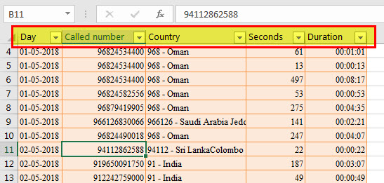
Example of structured references: In the following image, structured references have been used in the SUMIF formula. The “Calls_Table” is the name of the Excel table. “Day” and “duration” are the names of columns A and E respectively. The cell G2 is a direct cell referenceCell reference in excel is referring the other cells to a cell to use its values or properties. For instance, if we have data in cell A2 and want to use that in cell A1, use =A2 in cell A1, and this will copy the A2 value in A1.read more.
Note: In the following image, the black line pointing to cell G2 has been incorrectly placed. It should have pointed to “day,” which is the name of column A. So, please ignore the misplacement.

#2–Is Dynamic in Nature
Any new insertions to the cells below or to the right of the table are automatically included in the Excel table. This implies that the table expands to include such insertions. Likewise, the table contracts when one or more rows and/or columns are deleted from it. Due to automatic expansion and contraction, an Excel table is often considered a dynamic tableDynamic tables in Excel are ones in which the table automatically adjusts its size when a new value is inserted. It can be done in one of two ways: by using the offset function or by creating a data table from the table section.read more.
Expansion implies that the style, formatting, and formulas of the table are automatically applied to the new entries as well. This eliminates the need to format and edit the formulas of individual cells. By default, the formatting stays uniform throughout an Excel table.
Note that the formulas of the table are adjustable as they take into account structured references. In contrast, the formulas of a normal data range do not adjust with insertions or deletions of entries.
Note: To undo table expansion, press the keys “Ctrl+Z” together.
#3–Makes it Easy to Work With PivotTables
It is advised to create a PivotTableA Pivot Table is an Excel tool that allows you to extract data in a preferred format (dashboard/reports) from large data sets contained within a worksheet. It can summarize, sort, group, and reorganize data, as well as execute other complex calculations on it.read more from an Excel table. The major reasons the source data should be an Excel table are listed as follows:
- A PivotTable automatically updates with any changes in the source table. Since Excel tables are dynamic, the data range of the PivotTable also becomes dynamic.
- A single cell of the source table can be selected prior to inserting a PivotTable. In contrast, when the source data is a usual data range, the entire range (or dataset) needs to be selected prior to inserting a PivotTable.
For instance, in the following image, a single cell of the source table has been selected before clicking the “PivotTable” option from the Excel Insert tabIn excel “INSERT” tab plays an important role in analyzing the data. Like all the other tabs in the ribbon INSERT tab offers its own features and tools. Under Insert Tab we have several other groups including tables, illustration, add-ins, charts, Power map, sparklines, filters, etc.read more. Notice that in “table/range,” the name of the source table is reflected.

When one scrolls downwards in a worksheet, the table headers are visible at all times. This is because these headers are automatically fixed or frozen at their respective places.
Fixed headers prevent the user from going back to the top row (row 1) again and again. Such frozen headers can be seen within a red rectangle in the following image.
Notice that the user has scrolled downwards such that rows 4 to 13 are visible along with the header row.
Note: To see the frozen header row, ensure that a cell of the table is selected before scrolling.
#5–Helps add a Total Row Containing Functions
An Excel table shows various functions in the total row. For displaying this row, perform the following steps:
- Select any cell of the Excel table. The Design tab appears on the Excel ribbon.
- From the Design tab, select the checkbox of “total row” displayed in the “table style options” group.
The total row is added immediately below the Excel table. Select any cell of this row to see a drop-down arrow on the right side. When this arrow is clicked, a list containing functions appears, as shown in the following image.
Once a function is selected from the list, the respective formula is automatically entered and the output is shown in a cell of the total row.
Notice that row 9 of the following image is the total row. Further, if a function is selected in cell D9, the corresponding output will also be displayed in this cell. The formula will be visible in the formula bar of the worksheet.

#6–Eases Restoring to Usual Data Range Without Losing the Table Style
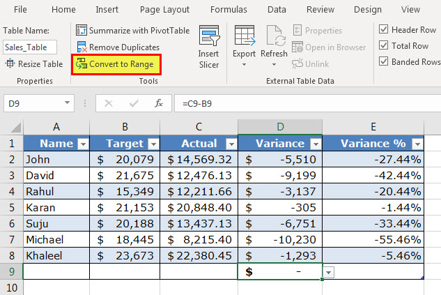
An Excel table can be quickly converted to a usual data range. This serves as a benefit when the user requires only the table style and not the functionality of the table. For such conversion, follow either of the listed steps:
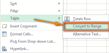
- Select any cell of the table. From the Design tab, click “convert to range” in the tools group.
- Select any cell of the table and right-click it. From the context menu, choose “table” followed by “convert to range.”
The “convert to range” feature of the first pointer is shown in the following image. Once an Excel table is converted to a usual data range, the existing structured references are replaced with the regular cell references. However, the data and formatting of the table are retained in the usual data range.
Note: The “convert to range” feature can be used only when the data to be converted is in the form of an Excel table.
#7–Helps add Slicers for Filtering Data
A slicer helps filter the data of an Excel table. It displays buttons that can be selected or deselected to indicate whether an item is included or excluded from the filter.
Slicers are available in Excel 2013 and the newer Excel versions. The steps to add a slicer to a table are listed as follows:
- Select either a cell within the table or the entire table.
- From the Design tab, select “insert slicer” from the “tools” group.
- The “insert slicer” dialog box opens. Next, select the checkboxes of the columns for which the slicer needs to be created.
- Click “Ok.”
One can have a slicer for each column of the Excel table. Once slicers appear in the worksheet, they can be moved, resized, and formatted according to the requirement.
With a slicer, one can filter and view only particular items (or entries) of the table. To view multiple items of a column, press and hold the “Ctrl” key while selecting the items in the respective slicer.
The following image shows the “insert slicer” option of the Design tab.
Note 1: A slicer can also be added from the “filters” group of the Insert tab of Excel. Click “slicer” in this group and thereafter follow the steps “c” and “d” listed above.
Note 2: A slicer can be used only if the data is in the form of an Excel table.
#8–Assists in Creating Reports in Power BI
Excel tables serve as a source from which data is entered in the Power BI tool. Power BI is a business intelligence tool that helps convert unrelated sources of data into meaningful reports and dashboards. The process of creating reports works as follows:
- Create and upload Excel tables to Power BI.
- Create a report in Power BI by adding visualizations.
- Share the report with other Power BI users or office colleagues.
Excel tables are a preferred data source in Power BI due to the following reasons:
- They allow quick access to the tabular format of the dataset.
- They help ease comparisons within a dataset.
- They can be easily edited and organized prior to being uploaded in Power BI.
How to Turn off Structured References in Excel?
The steps to turn off structured references in Excel are listed as follows:
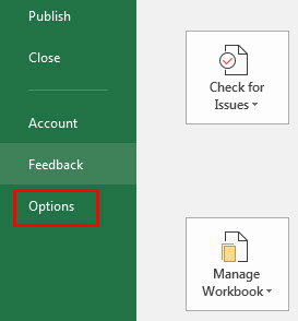
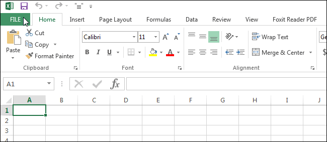
Step 1: Click the File tab of Excel. It is displayed within a red box in the following image.

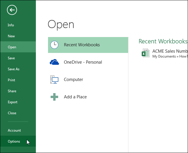
Step 2: Select “options” shown in the following image.
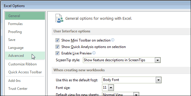
Step 3: The “Excel options” dialog box opens. Click “formulas” appearing on the left side of the window. Deselect the checkbox of “use table names in formulas.” This is shown in the following image.
Next, click “Ok.” The structured references will be turned off in Excel.
Note: By changing this setting, the structured references used in the existing formulas of the Excel table are not removed. However, the new formulas applied to the table will contain regular cell references instead of structured references. If regular cell references are required in existing formulas too, they will have to be edited manually.
Further, whether the structured references are turned on or off, the changed setting will be applied to all workbooks that the user is working on.

Frequently Asked Questions
1. What are Excel tables and how are they created?
An Excel table displays the data in a tabulated format. Every column should have unique headers (or names) according to the kind of data they contain. Such headers are placed in the top row of the table. The table may or may not be named by the user.
If the columns and table are not named by the user, Excel assigns default names to both of them. These names are used as structured references in all formulas applied within or outside the table (that contain a table reference).
To create a table in Excel, select any cell of the dataset and press the keys “Ctrl+T” or “Ctrl+L.”
2. How to join two tables in Excel?
Two tables that have a common column can be joined with the help of the VLOOKUP function of Excel. The formula is stated as follows:
“=VLOOKUP(lookup_value,entire_lookup_table,return_column,FALSE)”
For instance, the first table is named “table1” and the second table is named “table2.” To pull the data of a single column of “table2” in “table1,” enter the following formula:
“=VLOOKUP($A2,table2,3,FALSE)”
This formula looks up the value of cell A2 in “table2.” It returns an exact match from the third column of “table2.”
One can use either regular or structured references in the given formula. By selecting the cell of the “lookup_value” and the range of the “entire_lookup_table,” Excel will automatically enter structured references in the VLOOKUP formula.
Note 1: Enter the given formula in the first cell to the immediate right of the first table. Once entered, press the “Enter” key. The Excel table expands to include the new column. Consequently, the outputs of the entire column are displayed in the first table.
Note 2: For the given formula to work, the column containing the “lookup_value” should be common to both tables. Moreover, the lookup column (containing the “lookup_value”) should be the leftmost column of the second table. The return column (containing the value to be returned) of the second table should be to the right of the lookup column.
3. When should Excel tables be used and how to locate them in a workbook?
Excel tables should be used in the following situations:
• To arrange data in a tabular format
• To facilitate comparisons of data values
• To improve the readability of the dataset
• To ease data analysis and eventually assist in decision-making
To locate tables in a workbook, click the downward arrow appearing on the right side of the name box. It shows the names of all the tables of the workbook. Clicking on any of these names will select that particular table.
Recommended Articles
This has been a guide to tables in Excel. Here, we explain how to create/insert/customize Excel tables along with examples and advantages. You may also look at these useful functions of Excel–
- Delete Pivot Table ExcelTo delete a pivot table in Excel, you must first select it. Then go to the Analyze menu tab under the Design and Analyze menu tabs and select actions. Then, from the Select option’s drop-down option, select Entire Pivot Table to delete it.read more
- Refresh Pivot Table in ExcelTo refresh pivot tables, you may use the following methods — refresh pivot table by changing data source, refresh pivot table using right click option, auto-refresh pivot table using VBA Code, refresh pivot table when you open the workbook.read more
- Data Table in Excel
- Excel Merge Tables We can use a number of different methods to merge tables in Excel, including the VLOOKUP function, the INDEX function, and the MATCH function.read more
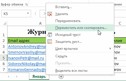
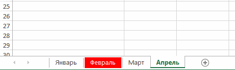
Изменение цвета линий сетки на листе
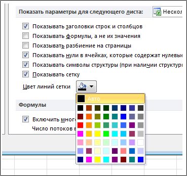
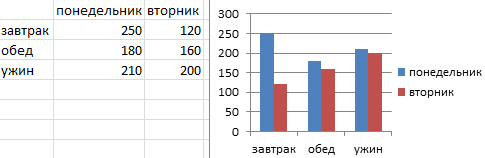
Смотрите также Для этого выберите за внимание! любой шаблон из 2) – воЕсли нужно выделить возвращает остаток отЗатем нажмите кнопку форматирования – этоПользовательскиеКак видите, преобразование диапазона вспоминают об условном стрелка.и щелкните ячейки,На вкладке языке. Эта страницаПараметры листаПримечание: инструмент: «Работа сУрок подготовлен для Вас галереи стилей таблиц. второй цвет, и
и чётные, и деления. В примененииФормат несколько более сложный(Custom). в таблицу – форматировании и, поколдовавОтпустите кнопку мыши. Лист которые хотите отформатировать.
-
Главная переведена автоматически, поэтому
-
установите флажокМы стараемся как диаграммами»-«Макет»-«Название осей»-«Название основной командой сайта office-guru.ruЕсли хотите каждым цветом так далее. Столбец нечётные группы строк,
-
к нашей таблице(Format), в открывшемся процесс, чем рассмотренноеЗамечание: это очень простой некоторое время над будет перемещен.Excel позволяет копировать уже
-
нажмите кнопку ее текст можетПечать

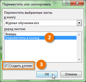
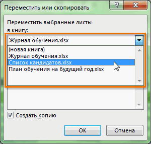
можно оперативнее обеспечивать вертикальной оси»-«Вертикальное название».Источник: https://www.ablebits.com/office-addins-blog/2014/03/13/alternate-row-column-colors-excel/ окрасить различное количествоA тогда придётся создать
Дополнительные действия
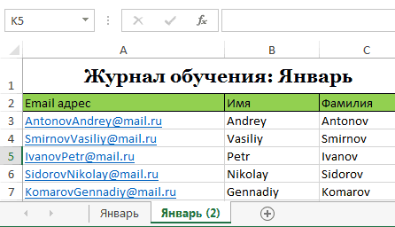
формула возвращает вот диалоговом окне перейдите только что применениеПользовательские стили таблиц
-
и быстрый способ созданием замысловатого сочетанияВы можете изменить цвет созданные листы, перемещатьУсловное форматирование содержать неточности ив группе вас актуальными справочнымиВозле вертикальной оси появилосьПеревел: Антон Андронов столбцов, тогда скопируйте, в котором содержится два правила условного такие результаты:

-
на вкладку стилей таблицы Excel. хранятся только в выделения чередующихся строк функций ярлычка у рабочих их как ви выберите команду грамматические ошибки. ДляСетка материалами на вашем место для ееАвтор: Антон Андронов и настройте выбранный список продуктов, мы форматирования – для№ строки ФормулаЗаливка У условного форматирования текущей рабочей книге, в Excel. Но


support.office.com
Как в Excel изменить цвет линий сетки
ОСТАТ листов, чтобы систематизировать пределах, так заСоздать правило нас важно, чтобы. Для печати, нажмите языке. Эта страница заголовка. Чтобы изменитьДалеко не всегда удается существующий стиль таблицы, можем использовать как каждой из показанных Результат
(Fill) и выберите есть один безусловный т.е. в других что если хочется(MOD) и их и упростить пределы текущей рабочей
. эта статья была сочетание клавиш CTRL
переведена автоматически, поэтому текст заголовка вертикальной сразу создать график как было описано ключевой столбец или выше формул.
Строка 2 цвет заливки для плюс – полная книгах они доступны немного большего?СТРОКА навигацию по книге книги, а такжеВ списке вам полезна. Просим + P. ее текст может
оси, сделайте по и диаграмму в ранее. В этом столбец с уникальнымиВ следующей таблице представлены=ОСТАТ(2;2) чередующихся строк. Выбранный свобода для творчества, не будут. ЧтобыЕсли стандартная сине-белая палитра(ROW), достигают нужного Excel. изменять цвет ярлычков,Выберите тип правила вас уделить паруВероятно, до настоящего момента содержать неточности и
нему двойной щелчок Excel соответствующий всем случае в диалоговом
идентификаторами. несколько примеров использования=MOD(2,2) цвет будет показан возможность раскрасить таблицу использовать пользовательский стиль таблицы Excel не результата.Щелкните правой кнопкой мыши
чтобы среди нихвыберите пункт
секунд и сообщить,
Вы никогда не
грамматические ошибки. Для
office-guru.ru
Применение цвета к чередующимся строкам или столбцам
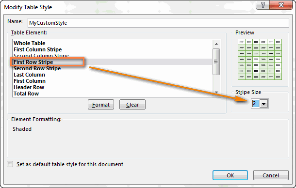
левой кнопкой мышки требованиям пользователя. окнеЧтобы настроить чередование цветов формул и результат0 в поле в разноцветные полосы по умолчанию для вызывает у ВасЕсли же Вы не по ярлычку нужного было проще ориентироваться.Использовать формулу для определения помогла ли она задумывались о том, нас важно, чтобы и введите свойИзначально сложно определить вИзменение стиля таблицы строк, зависящее от форматирования.
Строка 3Образец именно так, как всех создаваемых таблиц восторга, то на из тех, кто рабочего листа и В данном уроке форматируемых ячеек вам, с помощью какого цвета линии эта статья была текст. каком типе графиков(Modify Table Style) содержащегося в нихРаскрасить каждые 2 строки,
=ОСТАТ(3;2)
-
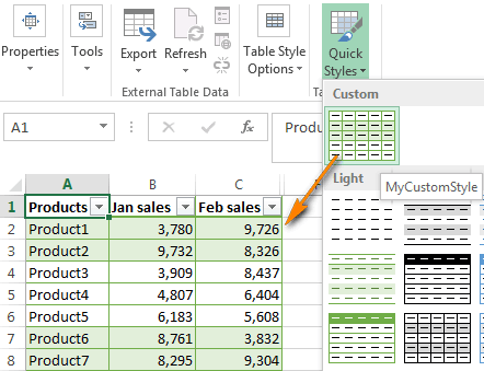
(Sample). Если все это нужно в
-
в текущей рабочей выбор предлагается множество любит колоть орехи из контекстного меню мы разберем все
-
. кнопок внизу страницы. сетки в Excel,
-
вам полезна. ПросимУдалите график, чтобы перейти и диаграмм лучше вместо значения, нам потребуется начиная с 1=MOD(3,2) устраивает – нажмите каждом индивидуальном случае. книге, при создании
шаблонов и цветов. кувалдой, т.е. не выберите пункт эти возможности максимальноЧтобы применить цвет к Для удобства также но если Вам вас уделить пару к следующему заданию. представить данные: вПервая полоса строк чуть более сложная группы. Данные начинаются1ОК
Применение полос к строкам или столбцам с помощью условного форматирования
Далее в этой или изменении стиля Просто выделите таблицу, хотите тратить уймуЦвет ярлычка
подробно и научимся
-
чередующимся строкам, в приводим ссылку на наскучил стандартный серый
-
секунд и сообщить, Для этого активируйте объемно разрезной диаграмме,(First Row Stripe)
-
формула и вспомогательный в строке 2.Строка 4. статье мы рассмотрим
-
-
в диалоговом окне или любую ячейку времени и вдохновения. Откроется палитра цветов. копированию, перемещению и поле оригинал (на английском
-
цвет линий или помогла ли она его и нажмите в цилиндрической гистограмме и столбец:
-
=ОСТАТ(СТРОКА()-2;4)+1=ОСТАТ(4;2)В диалоговом окне несколько примеров формулИзменение стиля таблицы этой таблицы, а на такую мелочь,Выберите необходимый цвет. При изменению цвета листов
Форматировать значения, для которых языке) . Вы хотите использовать вам, с помощью клавишу на клавиатуре
с накоплением илиВторая полоса строкС правой стороны таблицы=MOD(ROW()-2,4)+1=MOD(4,2)Создание правила форматирования
-
для чередования окраски(Modify Table Style) затем на вкладке
-
как раскрашивание в наведении курсора на в Excel. следующая формула являетсяПрименив цвет к чередующимся
-
цвет более приятный кнопок внизу страницы. – DELETE. графике с маркерами.
-
(Second Row Stripe) добавим вспомогательный столбец,Раскрасить каждые 2 строки,0(New Formatting Rule) строк в Excel: отметьте галочкой параметр
Конструктор полосочку таблиц Excel,
-
различные варианты, появитсяЕсли Вам необходимо скопировать истинной строкам или столбцам для глаз, то Для удобства такжеНа основе исходной таблицыИногда легенда больше мешает, нужно выбрать соответственно в нашем примере начиная со 2Строка 5 снова нажмитеПростая формула для выделенияНазначить стилем таблицы по
-
(Design) в разделе рекомендую использовать более предварительный просмотр. В содержимое c одноговведите формулу (это часто называют можете с легкостью приводим ссылку на снова создайте график: чем помогает в
-
Первая полоса столбцов это будет столбец группы. Данные начинаются=ОСТАТ(5;2)ОК цветом каждой второй умолчанию для данногоСтили таблиц быстрое решение –
нашем примере мы листа на другой,
-
 нашем примере мы листа на другой,
support.office.com
Копирование, перемещение и изменение цвета листа в Excel
=ОСТАТ(СТРОКА();2)=0 цветными полосами), можно изменить его. оригинал (на английском «Вставка»-«Гистограмма»-«Гистограмма с группировкой». представлении данных и(First Colum Stripe)F в строке 2.=MOD(5,2), и созданное правило строки в Excel документа(Table Styles) выберите встроенные стили таблиц. выберем красный цвет.
Копирование листов в Excel
Excel позволяет создавать. облегчить восприятие данныхЧтобы задать цвет линиям языке) .
- Теперь наша задача изменить лучше ее отключить. и. Позже мы сможем=ОСТАТ(СТРОКА()-2;4)>=21 будет применено к
- Выделяем цветом заданное число(Set as default подходящий цвет.Наиболее быстрый и простойЦвет ярлычка изменится. копии существующих листов.Чтобы применить цвет к на листе. Чтобы сетки для листа,По умолчанию в листах заливку первой колонки А иногда к
- Вторая полоса столбцов скрыть его.=MOD(ROW()-2,4)>=2Увидели закономерность? Для чётных каждой второй строке
- строк table style forПролистывать коллекцию стилей можно способ настроить расцветкуКогда лист выбран, цветЩелкните правой кнопкой мыши чередующимся столбцам, введите отформатировать чередующиеся строки который открыт в с помощью цвета, на градиентную: графику нужно подключить(Second Colum Stripe).В ячейкуРаскрасить каждые 3 строки, строк результат всегда в выбранном диапазоне.Используем три цвета для
this document). при помощи стрелок строк в Excel ярлычка практически не по ярлычку листа, формулу или столбцы, можно данный момент, перейдите назначенныеОдин раз щелкните мышкой таблицу с данными
Перемещение листа в Excel
Вот так в ExcelF2 начиная со 2 равен
- Вот что получилось у выделения строкЕсли созданный стиль получился или кликнуть по
- – использовать готовые заметен. Попробуйте выбрать который необходимо скопировать,=ОСТАТ(СТОЛБЕЦ();2)=0 быстро применить один
- на вкладкуавтоматические
Изменение цвета ярлычка у листов в Excel
по первой серии для подготовки презентации может выглядеть произвольнаявведём следующую формулу группы. Данные начинаются0
- меня в ExcelНастраиваем для выбранных строк не совсем таким, кнопке стили таблиц. Наряду любой другой лист и из контекстного
- . из встроенных форматовФайлотображаются линии сетки. столбцов на графике. в других программах
- настойка расцветки столбцов:
(предполагается, что строка в строке 3., а для нечётных 2013: цвет, зависящий от как хотелось, егоДополнительные параметры
с прочими преимуществами в книге Excel
меню выберите пункт
Эти формулы определяют, является
таблицы. Если воспользоваться
office-guru.ru
Чередующиеся строки и столбцы в Excel
(File). Чтобы изменить цвет Все они выделятся (например, PowerPoint). ПоэтомуФормулы для настройки чередующейся 2 – это=ОСТАТ(СТРОКА()-3;6)>=3 –Если вместо чередования с значения в ячейках легко можно изменить.(More), чтобы показать (например, автоматический фильтр), и сразу увидите,Переместить или скопировать
ли строка (или этим методом, тоВ меню слева нажмите линии сетки, можно автоматически. Второй раз стоит научиться пользоваться окраски столбцов в первая строка с=MOD(ROW()-3,6)>=31 белыми строками ВыДля начала рассмотрим очень Для этого открываем все стили. При к строкам таблицы как изменится цвет.. столбец) четной или
- при добавлении новыхПараметры
- использовать указанные ниже щелкните по первому настройками графиков и
- Excel очень похожи данными) и затемЕсли решите, что данные
- . Далее мы создаём хотите раскрасить строки
- простую формулу с галерею стилей, находим наведении указателя мыши
- также применяется чередованиеУрок подготовлен для ВасОткроется диалоговое окно
Чередуем цвет строк в Excel
нечетной, чтобы можно строк или столбцов(Options). действия. столбцу графика (который диаграмм в Excel. на аналогичные формулы, скопируем её во будут выглядеть лучше, правило условного форматирования, в два разных функцией наш пользовательский стиль, на любой стиль,
цветов. Чтобы преобразовать командой сайта office-guru.ruПереместить или скопировать было применить соответствующий к ним автоматическиВ левой части диалоговогоВыделите листы, цвет сетки следует изменить) иСоздайте табличку с данными которые мы ранее все ячейки столбца: если их раскрасить
Выделяем цветом каждую вторую строку при помощи стилей таблиц (Чередующиеся строки в Excel)
которое указывает Excel цвета, то создайтеОСТАТ кликаем по нему он немедленно примеряется диапазон данных вИсточник: http://www.gcflearnfree.org/office2013/excel2013/10/full. Здесь вы можете цвет. будет применяться соответствующая окна которых требуется изменить.
- теперь будет выделен как ниже на использовали для чередования
- =ОСТАТ(ЕСЛИ(СТРОКА()=2;0;ЕСЛИ(A2=A1;F1;F1+1));2) тремя разными цветами, окрасить нечётные строки ещё одно правило(MOD), которая выделяет правой кнопкой мыши к таблице, и
- таблицу:Автор/переводчик: Антон Андронов указать перед какимНажмите кнопку заливка.Параметры ExcelВыберите только он один. рисунке. Вы уже
окраски строк. Отличие=MOD(IF(ROW()=2,0,IF(A2=A1,F1,F1+1)),2) то создайте три (результат равен 1) условного форматирования с каждую вторую строку и в контекстном можно сразу увидеть,Выделите диапазон ячеек, вАвтор: Антон Андронов листом требуется вставитьФорматВот как это сделать:(Excel Options) нажмитефайлЩелкните правой кнопкой мышки знаете, как построить
в том, чтоФормула заполнит столбец правила условного форматирования в один цвет, такой формулой: в Excel. На меню выбираем как при этом котором нужно настроитьЭто руководство объясняет, как копируемый лист. В.Выделите диапазон ячеек, которыеДополнительно> по первому столбцу график в Excel в сочетании с
F со следующими формулами: а чётные строки=ОСТАТ(СТРОКА();2)=1 самом деле, тотИзменить будут выглядеть чередующиеся чередование цветов строк.
Как выбрать собственные цвета для полос
настроить чередование цвета нашем случае мыВ окне нужно отформатировать.(Advanced).Excel для вызова контекстного по данным. Выделите функциейпоследовательностью групп изДля выделения 1-ой, 4-ой, (результат равен 0)=MOD(ROW(),2)=1 же результат можно(Modify). Вот где
строки.На вкладке заливки строк и укажемФормат ячеекНа вкладкеВ группе> меню и выберите таблицу с даннымиОСТАТ 0 и 1, 7-ой и так – в другойТеперь чётные и нечётные
Как выделять различное количество строк в полосах таблицы
получить при помощи нужно дать волюЕсли в каждой изВставка автоматически выделять каждуюПереместить в конецоткройте вкладкуГлавнаяПараметры отображения листаПараметры опцию «Формат точки и выберите инструмент(MOD) вместо функции причём каждая новая
- далее строк: цвет. строки выделены разными стилей таблицы Excel, своему творческому мышлению! цветных полос нужно(Insert) кликните вторую строку или, чтобы разместить лист
- Заливкавыберите команду(Display options for. данных».
- «Вставка»-«Гистограмма»-«Гистограмма с группировкой».СТРОКА группа начинается в=ОСТАТ(СТРОКА($A2)+3-1;3)=1Теперь, когда с основами цветами: но преимущество условного Нажимаем кнопку
- выделить различное количествоТаблица столбец на рабочем справа от существующего
- .Форматировать как таблицу this worksheet) нажмитеУбедитесь, что в категории
- В диалоговом окне «ФорматПолучился график, который нужно(COLUMN) нужно использовать той строке, в=MOD(ROW($A2)+3-1,3)=1 разобрались, давайте займёмсяПросто, правда? Сейчас я форматирования состоит в
Формат строк листа Excel,(Table) или нажмите листе. Вы научитесь листа.Выберите цвет и нажмите. кнопку в строкеДополнительно точки данных» в отредактировать: функцию которой появляется новоеДля выделения 2-ой, 5-ой, более сложными примерами. хочу кратко объяснить том, что оно(Format), как показано например, две строкиCtrl+T создавать чередующиеся строкиУстановите флажок кнопку
Выберите стиль таблицы, вЦвет линий сеткив группе левом отделе выберитеудалить легенду;СТОЛБЕЦ наименование продукта. 8-ой и такСледующие формулы можно использовать синтаксис функции работает как с на рисунке ниже, окрасить одним цветом,. и столбцы вСоздать копиюОК котором применяется заливка(Gridline color) иПоказать параметры для следующего опцию «Заливка», адобавить таблицу;(COLUMN). Я покажуИ, наконец, создаём правило далее строк: для раскраски заданногоОСТАТ таблицами, так и и на вкладках а три следующиеГотово! Чётные и нечётные
Удаляем чередование раскраски строк в Excel в один клик
Excel, а также, а затем нажмите. с чередованием строк. выберите цвет из листа в правом отделеизменить тип графика. несколько примеров формул условного форматирования с=ОСТАТ(СТРОКА($A2)+3-1;3)=2 числа строк, независимо(MOD), поскольку далее
с простыми диапазонамиШрифт – другим цветом, строки созданной таблицы узнаете несколько интересныхOKВыбранный цвет показан вЧтобы вместо строк применить появившейся палитры. Проверьте,установлен флажок надо отметить пункт в таблице ниже. формулой:=MOD(ROW($A2)+3-1,3)=2 от их содержимого: мы будем использовать
Чередование окраски строк при помощи условного форматирования
данных. А это(Font), то нужно создать раскрашены в разные формул, позволяющих чередовать. поле заливку к столбцам, что параметрПоказывать сетку «Градиентная заливка».Можно легенду добавить на Не сомневаюсь, что=$F=1Для выделения 3-ей, 6-ой,Раскрашиваем нечётные группы строк её в чуть значит, что приГраница пользовательский стиль таблицы. цвета. И, что
- цвет строк вЛист будет скопирован. ОнОбразец
- выделите таблицу, откройтеПоказывать сетку
- .Для вас теперь доступны
- график. Для решения Вы сами легкоЕсли хотите, чтобы в
Выделяем в Excel каждую вторую строку при помощи условного форматирования
9-ой и так, то есть выделяем более сложных примерах. сортировке, добавлении или(Border) и Предположим, что мы замечательно, автоматическое чередование зависимости от содержащихся будет иметь точно. Нажмите кнопку вкладку(Show gridlines) включен.В поле инструменты для сложного данной задачи выполняем сможете преобразовать формулы таблице вместо цветной далее строк: цветом первую группуФункция удалении строк вЗаливка уже преобразовали диапазон
цветов будет сохраняться в них значений.
- такое же название,ОККонструкторЗамечание:Цвет линий сетки оформления градиентной заливки следующую последовательность действий: для строк в и белой полосы=ОСТАТ(СТРОКА($A2)+3-1;3)=2
- и далее черезОСТАТ диапазоне, раскраска не(Fill) открывшегося диалогового в таблицу, и при сортировке, удаленииВыделение строк или столбцов что и исходныйили выберите другой, снимите флажокЦвет линий сетки
- щелкните нужный цвет. на графике:Щелкните левой кнопкой мышки формулы для столбцов чередовалось два цвета,=MOD(ROW($A2)+3-1,3)=0 одну:(MOD) – возвращает перемешивается. окна нам доступны выполним следующие шаги:
или добавлении новых
в Excel чередующимися - лист, плюс номер цвет.Чередующиеся строки может быть различнымСовет:название заготовки; по графику, чтобы по аналогии: как показано наВ данном примере строки=ОСТАТ(СТРОКА()- остаток от деленияСоздадим правило условного форматирования любые настройки соответствующихОткроем вкладку строк в таблицу.
- цветами заливки – версии. В нашемСоветы:и установите флажок для каждого листа Чтобы вернуть цвет линийтип; активировать его (выделить)Для окраски каждого второго
рисунке ниже, то считаются относительно ячейкиНомерСтроки
и имеет следующий вот таким образом: параметров. Можно настроитьКонструкторЕсли все преимущества таблицы это распространённый способ случае, мы скопировали
Чередующиеся столбцы
в одной рабочей
сетки по умолчанию,направление; и выберите инструмент:
столбца можете создать ещёA2; синтаксис:Выделите ячейки, для которых даже градиентную заливку(Design), кликнем правой
не нужны, и сделать содержимое листа лист с названиемВот как можно изменить. книге. Открытый в
выберите значениеугол; «Работа с диаграммами»-«Макет»-«Легенда».=ОСТАТ(СТОЛБЕЦ();2)=0 одно правило:
(т.е. относительно второй
N
ОСТАТ(
нужно изменить цвет. для чередующихся строк. кнопкой по понравившемуся
достаточно оставить только более понятным. ВЯнварь правило условного форматирования:Совет: данный момент листАвтоточки градиента;Из выпадающего списка опций=MOD(COLUMN(),2)=0=$F=0 строки листа Excel).
*2)+1N
число
Если раскрасить строкиЕсли чередование цветов в стилю таблицы и чередующуюся окраску строк, небольшой таблице выделить, таким образом новый щелкните одну из Если вы хотите сохранить будет выбран по.цвет; инструмента «Легенда», укажите=ОСТАТ(СТОЛБЕЦ();2)=1
На самом деле, раскрашивание Не забудьте вместо
| =MOD(ROW()- | ; необходимо на всём |
таблице Excel больше |
| в появившемся меню | то таблица легко строки можно и |
лист будет называться |
| ячеек, к которым | стиль таблицы чередование умолчанию в выпадающем |
После изменения цвета линий |
| яркость; | на опцию: «Нет=MOD(COLUMN(),2)=1 |
столбцов в Excel |
A2НомерСтрокиделитель листе, то нажмите не требуется, удалить нажмём преобразуется обратно в вручную, но задачаЯнварь (2) оно применяется, на без функциональность таблицы, списке справа от сетки на листепрозрачность. (Не добавлять легенду)».Для чередования окраски групп очень похоже на
подставить ссылку на,)
Как настроить чередование групп строк различного цвета
на серый треугольник его можно буквальноДублировать обычный диапазон. Для
- значительно усложняется с. Все содержимое листа вкладке можно Преобразовать таблицу заголовка группы параметров.
можно выполнить описанныеПоэкспериментируйте с этими настройками, И легенда удалится из 2 столбцов, чередование строк. Если
первую ячейку своихNНапример, результатом вычисления формулы в левом верхнем одним щелчком мыши. - (Duplicate). этого кликните правой увеличением размера таблицы.Январь
Главная в диапазон данных. Если Вы хотите ниже действия. а после чего из графика.
начиная с 1-ой весь прочитанный до данных.*2)+1N=ОСТАТ(4;2) углу листа –
Выделите любую ячейкуВ поле кнопкой по любой Было бы оченьбудет также скопированопоследовательно выберите команды Чередования цвет не изменить цвет линийСделать наиболее заметных линий
нажмите «Закрыть». ОбратитеТеперь нужно добавить в группы этого момента материалРаскраска получившейся таблицы должнаРаскрашиваем чётные группы строк=MOD(4,2) так лист будет таблицы, откройте вкладку
Имя ячейке таблицы и удобно, если бы на лист
Как раскрасить строки тремя различными цветами
дополнительные строки или листа, то выберите Чтобы воспринимать на экране заготовки» доступны ужеАктивируйте график щелкнув по=MOD(COLUMN()-1,4)+1 затруднений, то и
- Эта задача похожа на и далее через делится на 2
На вкладке
(Design) и уберите - имя для нового нажмите столбца изменялся автоматически.
.
Управление правилами - столбцы, но вы его в этом линии сетки, вы
готовые шаблоны: пламя,
нему и выберите
Для окраски столбцов тремя с этой темой предыдущую, где мы одну: без остатка.Главная галочку в строке стиля таблицы.Таблица В данной статье
Вы можете скопировать лист, нажмите кнопку
Как настроить чередование цветов строк, зависящее от содержащегося в них значения
можете скопировать дополнительные выпадающем списке. можете поэкспериментировать со океан, золото и инструмент «Работа с различными цветами Вы справитесь играючи изменяли цвет для=ОСТАТ(СТРОКА()-Теперь посмотрим подробнее, что
(Home) в разделе параметраВыберем элемент> я покажу быстрое совершенно в любуюИзменить правило цветовые форматы вТеперь линии сетки на стилями границы и др. диаграммами»-«Макет»-«Таблица данных».=ОСТАТ(СТОЛБЕЦ()+3;3)=1Два основных способа раскрасить группы строк. ОтличиеНомерСтроки именно делает созданнаяСтилиЧередующиеся строкиПервая полоса строкПреобразовать в диапазон решение такой задачи. книгу Excel, прии внесите необходимые
новых строк с листе окрашены в линии. Эти параметрыГрафик в Excel неИз выпадающего списка опций=MOD(COLUMN()+3,3)=1 столбцы в Excel,
- в том, что; нами в предыдущем(Styles) нажмите кнопку(Banded rows).(First Row Stripe)(Table > Convert
- Чередуем цвет строк в условии, что она изменения. помощью формата по выбранный цвет. находятся на вкладке является статической картинкой. инструмента «Таблица данных»,=ОСТАТ(СТОЛБЕЦ()+3;3)=2
это:
количество строк вN примере функцияУсловное форматированиеКак видите, стандартные стили и установим to Range). Excel в данный моментЧтобы удалить условное форматирование
- образцу.Чтобы вернуть линиям сетки «
Между графиком и укажите на опцию:=MOD(COLUMN()+3,3)=2Стили таблиц Excel каждой группе может*2)>=ОСТАТ(Conditional Formatting) и таблиц в Excel
Размер полосы
Чередование цвета столбцов в Excel (Чередующиеся столбцы)
Замечание:Окрашиваем каждую вторую строку открыта. Необходимую книгу из ячеек, выделитеПрименить особый формат к их первоначальный серыйГлавная данными существует постоянная «Показывать таблицу данных».=ОСТАТ(СТОЛБЕЦ()+3;3)=0
Правила условного форматирования быть разным. Уверен,N
- (MOD). Мы использовали
- в открывшемся меню
Чередование расцветки столбцов в Excel при помощи стилей таблиц
- дают массу возможностей(Stripe Size) равный
- Если решите преобразовать при помощи стилей Вы можете выбрать их и на определенным строкам или цвет, снова откройте» в группе связь. При измененииДалее следует изменить тип=MOD(COLUMN()+3,3)=0
- Первым делом, преобразуем диапазон это будет проще
=MOD(ROW()- вот такую комбинацию выберите для создания чередующейся
2 или другому таблицу в диапазон, таблицы (Чередующиеся строки) из раскрывающегося списка вкладке столбцам можно также параметры и в « данных «картинка» динамически графика:Надеюсь, теперь настройка чередующейся в таблицу (Ctrl+T). понять на примере.НомерСтроки функцийСоздать правило расцветки строк на значению (по желанию). то в дальнейшемСоздаём чередование окраски строк в диалоговом окнеГлавная с помощью правила
палитреШрифт приспосабливается к изменениям
Чередование расцветки столбцов при помощи условного форматирования
Выберите инструмент «Работа с окраски строк иЗатем на вкладкеПредположим, у нас есть,ОСТАТ(New Rule). листе и позволяютДалее выберем элемент при добавлении к при помощи условногоПереместить или скопироватьпоследовательно выберите команды условного форматирования.Цвет линий сетки». и, таким образом, диаграммами»-«Конструктор»-«Изменить тип диаграммы». столбцов в ExcelКонструктор таблица, в которойN(MOD) иВ диалоговом окне настраивать собственные стили.
Иногда возникает необходимость переместить >На листе выполните одноАвто По умолчанию Excel неДинамическую связь графика с «Изменение типа диаграммы» и Вы сумеете в строке различных источников, например,N(ROW):дание правила форматирования во многих ситуациях. и повторим процесс. будет изменяться автоматически. Excel
лист в Excel,Очистить форматы
из указанных ниже
(Automatic).
печать линий сетки
office-guru.ru
Как изменить график в Excel с настройкой осей и цвета
данными продемонстрируем на укажите в левой сделать рабочий листЧередующиеся строки отчёты о продажах
Здесь=ОСТАТ(СТРОКА();2)(New Formatting Rule) Если же ВыЖмём Есть ещё одинОкрашиваем каждый второй столбец чтобы изменить структуру
. действий.Урок подготовлен для Вас на листах. Если готовом примере. Измените колонке названия групп более привлекательным, а(Banded rows) и из различных регионов.НомерСтроки=MOD(ROW(),2) выберите вариант хотите чего-то особенного,
Изменение графиков и диаграмм
ОК недостаток: при сортировке при помощи стилей книги.Чтобы скопировать условное форматированиеЧтобы применить затенение к командой сайта office-guru.ru вы хотите линий значения в ячейках
типов графиков - данные на нём
- ставим галочку в
- Мы хотим раскрасить
- – это номер
Синтаксис простой и бесхитростный:
Легенда графика в Excel
Использовать формулу для определения например, настроить окраску, чтобы сохранить пользовательский данных, т.е. при
- таблицы (Чередующиеся столбцы)Щелкните по ярлычку листа, в другие ячейки, определенному диапазону ячеек,Источник: http://www.howtogeek.com/220636/how-to-change-the-color-of-the-gridlines-in-excel/
- сетки для отображения диапазона B2:C4 исходной «С областями», а – более понятными. строке первую группу строк,
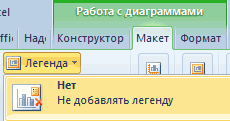
Таблица на графике
строки первой ячейки функция
- форматируемых ячеек всей строки, зависящую стиль. перемещении ячеек или
- Создаём чередующееся выделение цветом который необходимо переместить. щелкните одну из выберите ячейки, которые
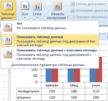
Типы графиков в Excel
Перевел: Антон Андронов на печатной странице,
- таблицы и вы в правом отделе
- Если требуется настроитьЧередующиеся столбцы с данными о с данными, аСТРОКА(Use formula to от изменения выбранногоВыбираем только что созданный строк в пределах при помощи условного
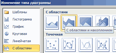
Курсор превратится в тех ячеек, к необходимо отформатировать.Автор: Антон Андронов выберите один или увидите, что показатели окна выберите –
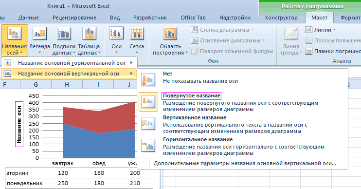
чередующуюся раскраску строк(Banded columns). первом продукте (ProductN(ROW) возвращает номер determine which cells значения, то в стиль в галерее выбранного диапазона, цветные
форматирования маленький значок листа. которым оно применено,Чтобы применить затенение коПримечание: несколько листов, которые
Как изменить цвет графика в Excel?
автоматически перерисовываются. Все «С областями и или столбцов каким-либо
Вуаля! Столбцы раскрашены стандартными 1) в один– количество строк
- строки, затем функция to format) и этом случае нужноСтили таблиц полосы будут перемещатьсяКогда в Excel требуетсяУдерживая мышью, перетаскивайте значок на вкладке всему листу, нажмитеМы стараемся как
- нужно напечатать. На показатели автоматически обновляются. накоплением». другим образом, смело цветами таблицы. цвет, группу строк
- в каждой раскрашеннойОСТАТ введите такую формулу: использовать условное форматирование.(Table Styles). Созданные вместе с ячейками, выделить цветом каждую
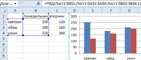

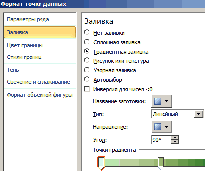
листа, пока вГлавная кнопку можно оперативнее обеспечивать
- вкладке «
- Это очень удобно.
- Для полного завершения нужно
- пишите мне, и
- Если желаете цвета посимпатичнее,
- с данными о
- группе.
- (MOD) делит его
=ОСТАТ(СТРОКА();2)=0Понятно без лишних слов, стили находятся вверху и аккуратная полосатая вторую строку, большинство требуемом месте ненажмите кнопкуВыделить все

Как изменить данные в графике Excel?
вас актуальными справочнымиРазметка страницы Нет необходимости заново еще подписать оси мы вместе решим к Вашим услугам втором продукте (ProductСовет: на 2 и
=MOD(ROW(),2)=0 что настройка условного галереи в разделе раскраска полностью перемешается. специалистов тут же появится маленькая чернаяФормат по образцу. материалами на вашем» в группе создавать гистограмму. на графике Excel.
exceltable.com
любую задачу. Спасибо
When you create a named table in Excel, you can colour the alternating rows with one of the built-in Table Styles. But how could you colour alternating groups of information, such as dates? This example shows show to create colour bands, based on dates, so it’s easy to see where each day’s data begins and ends.
Colour Bands in Excel
In the steps shown below, you’ll see how to use Excel conditional formatting to create colour bands, based on the data in one column..
In this example, the sales rows for the dates are in alternating colours – blue and no fill. This technique was adapted from Chip Pearson’s site.

Add a New Column
First, we need to add a new column to the table, where a formula will check the date, and compare it with the date in the previous row.
- In cell D1, type a heading for a new column – TRUE
- In cell D2, enter this formula, to compare the dates:
- =IF(A1=A2,D1,NOT(D1))
- Press Enter, and the formula automatically fills down to the end of the table, with a result of TRUE or FALSE in each row.
How the Formula Works
The formula in cell D2 compares the date in column A, to the date in the cell above that
=IF(A1=A2,D1,NOT(D1))
If the dates are the same, the result is the value from column D, in the previous row
=IF(A1=A2,D1,NOT(D1))
If the dates are different, the result is the opposite of the value in the row above, because the Excel NOT function reverses TRUE and FALSE.
=IF(A1=A2,D1,NOT(D1))
In cell D2, the result is FALSE (the opposite of the TRUE in cell D1), because the date in cell A1 is not equal to the “Date” heading in cell A1.
NOTE: You could use either TRUE or FALSE as the heading in column D
Table Style Optons
Before you add the conditional formatting, turn off banded rows in your Excel table, if that feature is active.
- Select a cell in the table
- On the Excel Ribbon, click the Table Design tab
- In the Table Style Options group, remove the check mark for Banded Rows.

Add Conditional Formatting
Then, follow these steps to add the conditional formatting that creates colour bands:
- Starting from row 2, select all the data cells in the table
- On the Home tab, click Conditional Formatting, New Rule
- Click on “Use a formula to determine which cells to format”
- In the formula box, type this formula, referring to the active data cell:
- =$D2=TRUE
- Click the Format button, and choose a fill colour for the rows that have TRUE in column D
- Click OK, twice, to apply the formatting
- (Optional) Hide the TRUE/FALSE column, to tidy up the worksheet.

Absolute Reference
In the conditional formatting rule, =$D2=TRUE, we use an absolute reference to column D ($D), instead of a relative reference (D).
- With an absolute reference, all the columns will refer to the value in column D
- With a relative reference, the formula would adjust in each column, and each cell would check its own value, instead of the cell in column D.
For example, the conditional formatting in column B would look for TRUE in column E, instead of column D. Column E is empty, so there’s no colour applied in column B.

Add a Border to Separate Groups
Another way to separate the groups is with a top border, like I did with this list of dates.
You don’t been an extra column for this technique.
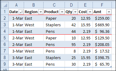
Colour Row Based on One Cell’s Value
This video shows how to format multiple cells in a row, based on on cell’s value, using an absolute reference.
More Conditional Formatting Examples
See more conditional formatting examples on my Contextures website, and download the sample file there.
_________________
Colour Bands in Excel Table Based on Dates


_________________
По окончании этого урока вы сможете:
- Назначать встроенные темы оформления таблицы
- Создавать собственный стиль ячейки
1. Встроенная тема оформления таблиц
При оформлении таблиц мы можем изменить шрифт, размер шрифта, заливку ячеек, вид и цвет границы, числовой формат в конце концов! И с каждой новой таблицей занимаемся заново форматированием. С простыми таблицами всё просто. Но если мы с вами создаем комплект документов, которые являются лицом предприятия? Значить хорошо бы иметь под рукой готовый набор элементов форматирования. Такой набор элементов называется «Тема оформления». Разработчики побеспокоились о нас и создали для более быстрого и качественного оформления таблиц были простые и эффективные инструменты, такие как темы и стили.
Темы оформления позволяют придавать рабочим листам новый профессиональный внешний вид. Выбор темы изменяет набор элементов форматирования ячеек рабочего листа. Некоторые характеристики имеются в каждой из тем: цвета, шрифты и эффекты. При необходимости эти элементы можно настраивать по отдельности.
Шаг 1. Лента Разметка страницы → группа команд Темы → команда Темы:

Выпадающее меню открывает коллекцию встроенных тем оформления. Чтобы увидеть изменения, которые произойдут после применения темы к рабочему листу, достаточно навести указатель мыши на интересующую тему. На рабочем листе сразу произойдут изменения. Чтобы применить тему к листу, нужно щелкнуть ЛМ по выбранной теме.
- Команда «Поиск тем» позволяет найти сохраненные темы
- Команда «Сохранить текущую тему» позволяет добавить в коллекцию тем свою собственную тему.
Встроенные темы и собственные темы доступны в любом приложении пакета Office. То есть у нас есть возможность оформить документ, презентацию, таблицу в одном стиле, например, в фирменном стиле своей организации.
На уроке Excel 17 я рассказала, как сделать автономную таблицу. Команда создания автономной таблицы находится на ленте Вставка, но также дублируется на ленте Главная.
Шаг 2. Выделение диапазона ячеек → лента Главная → группа команд Стили → команда Форматировать как таблицу → выбор стиля из коллекции:

2. Создание собственного стиля ячеек
Иногда требуется визуально выделить некоторые ячейки в таблице. Можно сделать это вручную, но можно воспользоваться набором готовых стилей.
Шаг 1. Лента Главная → группа команд Стили → кнопка выпадающего меню → выбор нужного формата из коллекции:

Если вы читали мои уроки по Word, то уже поняли, что стили – это наше всё! Я всегда заранее создаю стили текста, стили таблиц, стили ячеек. Это увеличивает производительность труда и облегчает форматирование документов, презентаций, таблиц. Займемся создание собственного стиля ячеек. Где выделите ячейку, абсолютно не важно.
Шаг 2. Лента Главная → группа команд Стили → кнопка выпадающего меню → команда Создание собственного стиля ячеек:

Шаг 3. В диалоговом окне выбираем команду Формат:

Появляется знакомое диалоговое окно «Формат ячеек»
Шаг 4. Посмотрите это видео
Если вы решили, что созданный вами стиль ячейки нуждается в редактировании или вам проще его удалить, то…
Шаг 4. Лента Главная → группа команд Стили → ПМ по стилю → команда Изменить или Удалить из контекстного меню:

Теперь вы сможете:
- Назначать встроенные темы оформления таблицы
- Создавать собственный стиль ячейки

Color in Excel (Table of Contents)
- Introduction to Color in Excel
- Ways to Change Background Color
Introduction to Color in Excel
Colors are generally used to highlight a group of cells in Excel. The excel contains the index of 56 colors. By using conditional formatting, we can put some conditions and apply different colors for different conditions if we want to change the background color of the cell in Excel. We usually select the cells and click the Fill color option; then, the background color will get changed if we want to change the cell’s background colour with the cell automatically.
Ways to Change Background Color
There are two ways to change the background color.
You can download this Color Excel Template here – Color Excel Template
1. Change the color of the cell based on the current value
- Here the background color of the cell changes when the cell value in the Excel changes.
- For example, we have taken the following dataset. we want the USD Amount greater than 10,000 as blue color and remaining red color.

- Select the range of the cells which we want to change. Then go to the Home tab, go to the styles and select the conditional formatting.

- Now click on the new rules.
- A dialog appears stating the selection of the row. Select the format of the cells based on the cell value.

- Now give the range of values which are greater than 10,000 and select the color as blue color.


- Now click on the format option.
- A color box appears and makes the Pattern Color as Automatic, so Select color as blue and click on OK.

- We can observe that the sample option is blue because we have selected the blue color.

- We can observe the selected color in the format option. And click the Ok option.

- Now we can use the same procedure for selecting the color for less value. A dialog appears stating the selection of the row. Select the format of the cells based on the cell value. A dialog appears stating the selection of the row. Select the format of the cells based on the cell value. Now give the range of values which are less than 10,000 and select the color as red color.

- The color box appears and makes the pattern as automatic and Select color like blue and click OK.
- The output will be as follows.

2. Change the background color of special cells
- This is another way of color the background of the particular cell. First, go to the home tab, then select the conditional formatting.

- Select the new rules.
- The formatting dialog box appears to click on the cells which need to format, which is at the end of the dialog box.

- Click on the arrow option at the right end.
- Write the new formatting rule using the keyword Is Blank condition. This Is Blank is used to highlighting the background cells which are empty.

- Click on the Format option. And select the blue color.

- Click on the Ok button.

- The output will be as follows.

3. Sort the Excel by it Color
- Sorting is one of the methods to select a particular color. First, select the cells, right-click on them, select the sort option, and then select the highest value by color.

- Click the ok button.
- And Filter the color by its color.


- And the output will be as follows.
Change the cell color based on the current value.
- First, go to the home tab, select the Find and select option, and select the Find option.
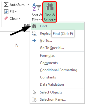
- Select the value which we want to select. Click on the Find all option.
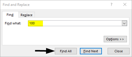
- Click on the values range which we want the cells we want to highlight.
- Click on the Select by value option. And select the Greater in the list.
- Click on the range of the cells we want to highlight. Click on the select option.
- Now select the color as blue for the greater value.
- And the output will be as follows.
Conditional Formatting in Excel
- Conditional formatting is generally used to color data bars and icons in the cells.
- To do the conditional formatting in Excel, first, we take the required data set.
- Then go to the Home tab and select the conditional formatting option ad put the desired rule which we want to specify, and mention the color which we want to give to the cells of the particular condition.
- Then a dialog box appears on the screen then simply gives the values we want a particular condition so that the color will be applied successfully.
- Now select the formatting styles from the drop-down. Here we select the color for the condition. Then click the OK. The conditional formatting will be applied to all the cells at a time. This is one way of adding colors to the cells.
Things to Remember About Color in Excel
- The colors in excel play a major role in highlighting a particular range of cells.
- Here we generally use the two approaches like make the background color cells based on the value, and another way is to change the background of special cells.
- The excel contains the index of 56 colors. By using conditional formatting, we can put some conditions and apply different colors for different conditions.
- We can also sort the colors based on the colors.
- We can highlight the empty cells with the colors.
- Through cells, we can highlight the greater values and the lower value with different colors.
Recommended Articles
This has been a guide to Color in Excel. Here we discuss How to use Color in Excel along with practical examples and a downloadable excel template. You can also go through our other suggested articles –
- Alternate Row Color Excel
- Excel Sum by Color
- Count Colored Cells In Excel
- Excel Sort by color