
You can highlight data in cells by using Fill Color to add or change the background color or pattern of cells. Here’s how:
-
Select the cells you want to highlight.
Tips:
-
To use a different background color for the whole worksheet, click the Select All button. This will hide the gridlines, but you can improve worksheet readability by displaying cell borders around all cells.
-

-
-
Click Home > the arrow next to Fill Color
, or press Alt+H, H.
-
Under Theme Colors or Standard Colors, pick the color you want.
To use a custom color, click More Colors, and then in the Colors dialog box select the color you want.
Tip: To apply the most recently selected color, you can just click Fill Color
. You’ll also find up to 10 most recently selected custom colors under Recent Colors.

 , or press Alt+H, H.
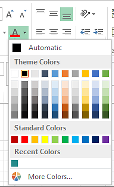
Apply a pattern or fill effects
When you want something more than a just a solid color fill, try applying a pattern or fill effects.
-
Select the cell or range of cells you want to format.
-
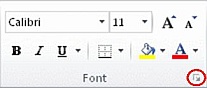
Click Home > Format Cells dialog launcher, or press Ctrl+Shift+F.
-
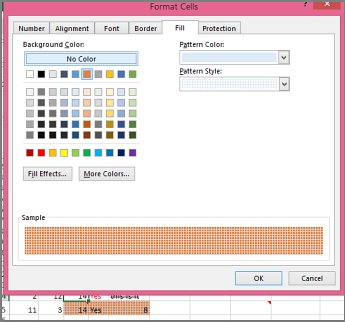
On the Fill tab, under Background Color, pick the color you want.
-
To use a pattern with two colors, pick a color in the Pattern Color box, and then pick a pattern in the Pattern Style box.
To use a pattern with special effects, click Fill Effects, and then pick the options you want.
Tip: In the Sample box, you can preview the background, pattern, and fill effects you selected.
Remove cell colors, patterns, or fill effects
To remove any background colors, patterns, or fill effects from cells, just select the cells. Then click Home > arrow next to Fill Color, and then pick No Fill.
Print cell colors, patterns, or fill effects in color
If print options are set to Black and white or Draft quality — either on purpose, or because the workbook has large or complex worksheets and charts that caused draft mode to be turned on automatically — cells won’t print in color. Here’s how you can fix that:
-
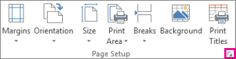
Click Page Layout > Page Setup dialog box launcher.
-
On the Sheet tab, under Print, uncheck the Black and white and Draft quality check boxes.
Note: If you don’t see colors in your worksheet, it may be that you’re working in high contrast mode. If you don’t see colors when you preview before you print, it may be that you don’t have a color printer selected.
If you’d like to highlight text or numbers to make the data more visible, try either changing the font color or add a background color to the cell or range of cells like this:

-
Select the cell or range of cells for which you want to add a fill color.
-
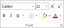
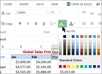
On the Home tab, click Fill Color, and pick the color you want.
Note: Pattern fill effects for background colors are not available for Excel for the web. If you apply any from Excel on your desktop, it won’t appear in the browser.
Remove fill color
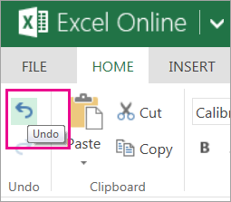
If you decide that you don’t want the fill color immediately after you added it, just click Undo.
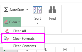
To remove the fill color at a later time, select the cell or cell range you want to change, and click Clear > Clear Formats.
Let’s say that one of our tasks is to entering of the information about: did the ordering to a customer in the current month. Then on the basis of the information you need to select the cell in color according to the condition: which from customers have not made any orders for the past 3 months. For these customers you will need to re-send the offer.
Of course it’s the task for Excel. The program should automatically find such counterparties and, accordingly, to color ones. For these conditions we will use to the conditional formatting.
The filling cells with dates automatically
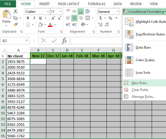
At first, you need to prepare to the structure for filling the register. First of all, let’s consider to the ready example of the automated register, which is depicted in the picture below. Today date 07.07.2018:
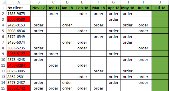
The user to need only to specify, if the customer have made an order in the current month, in the corresponding cell you should enter the text value of «order». The main condition for the allocation: if for 3 months the contractor did not make any order, his number is automatically highlighted in red.
Presented this decision should automate some work processes and to simplify to the visual data analysis.
The automatic filling of the cells with the relevant dates
At first, for the register with numbers of customers we will create to the column headers with green and up to date for months that will automatically display to the periods of time. To do this, in the cell B1 you need to enter the following formula:
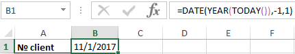
How does the formula work for automatically generating of the outgoing months?
In the picture, the formula returns the period of time passing since the date of writing this article: 17.09.2017. In the first argument in the function DATE is the nested formula that always returns the current year to today’s date thanks to the functions: YEAR and TODAY. In the second argument is the month number (-1). The negative number means that we are interested in what it was a month last time. The example of the conditions for the second argument with the value:
- 1 means the first month (January) in the year that is specified in the first argument;
- 0 – it is 1 month ago;
- -1 – there is 2 months ago from the beginning of the current year (i.e. 01.10.2016).
The last argument-is the day number of the month, which is specified in the second argument. As a result, the DATE function collects all parameters into a single value and the formula returns to the corresponding date.
Next, go to the cell C1 and type the following formula:
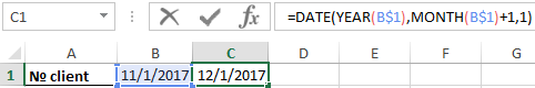
As you can see now the DATE function uses the value from the cell B1 and increases to the month number by 1 in relation to the previous cell. As the result is the 1 – the number of the following month.
Now you need to copy this formula from the cell C1 in the rest of the column headings in the range D1:AY1.
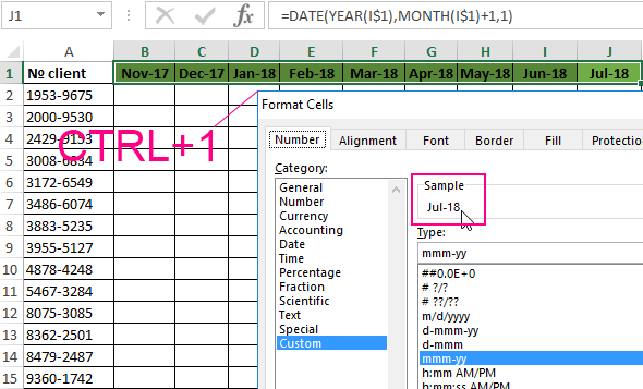
To highlight to the cell range B1:AY1 and select to the tool: «HOME»-«Cells»-«Format Cells» or just to press CTRL+1. In the dialog box that appears, in the tab «Number» in the section «Category» you need to select the option «Custom». In the «Type:» to enter the value: MMM. YY (required the letters in upper register). Because of this, we will get to the cropped display of the date values in the headers of the register, what simplifies to the visual analysis and make it more comfortable due to better readability.
Please note! At the onset of the month of January (D1), the formula automatically changes in the date to the year in the next one.
How to select the column by color in Excel under the terms
Now you need to highlight to the cell by color which respect of the current month. Because of this, we can easily find the column in which you need to enter the actual data for this month. To do this:
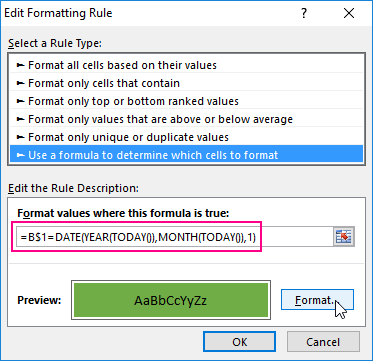
- To select the range of the cells B2:AY15 and select the tool: «HOME» -«Styles» -«Conditional Formatting»-«New Rule». And in the appeared window «New Formatting Rule» you need to select the option: «Use a formula to determine which cells to format»
- In the input field to enter the formula:
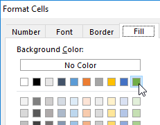
- Click «Format» and indicate on the tab «Fill» in what color (for example green) will be the selected cells of the current month. Then on all Windows for confirmation to click «OK».
The column under the appropriate heading of the register is automatically highlighted in green accordingly to our terms and conditions:
How does the formula highlight of the column color on a condition work?
Due to the fact that before the creation of the conditional formatting rule we have covered all the table data for inputting data of register, the formatting will be active for each cell in the range B2:AY15. The mixed reference in the formula B$1 (absolute address only for rows, but for columns it is relative) determines that the formula will always to refer to the first row of each column.
Automatic highlighting of the column in the condition of the current month
The main condition for the fill by color of the cells: if the range B1:AY1 is the same date that the first day of the current month, then the cells in a column change its colors by specified in conditional formatting.
Please note! In this formula, for the last argument of the function DATE is shown 1, in the same way as for formulas in determining the dates for the column headings of the register.
In our case, is the green filling of the cells. If we open our register in next month, that it has the corresponding column is highlighted in green regardless of the current day.
The table is formatted, now we are filling it with the text value of the «order» in a mixed order of clients for current and past months.
How to highlight the cells in red color according to the condition
Now we need to highlight in red to the cells with the numbers of clients who for 3 months have not made any order. To do this:
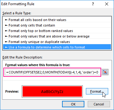
- Select the range of the cells A2:A15 (that is, the list of the customer numbers) and select to the tool: «HOME»-«Styles»-«Conditional formatting»-«Create rule». And in the window that appeared «Create a formatting rule» to select the option: «Use the formula for determining which cells to format».
- This time in the input box to enter the formula:
- To click «Format» and specify the red color on the tab «Fill». Then on all Windows click «OK».
- Fill the cells with the text value of «order» as in the picture and look at the result:
The numbers of customers are highlighted in red, if in the row has no have the value «order» in the last three cells for the current month (inclusively).
The analysis of the formula for the highlighting of cells according to the condition
Firstly, we will do by the middle part of our formula. The SHIFT function returns a range reference shifted relative to the basic range of the certain number of rows and columns. The returned reference can be a single cell or a range of cells. Optionally, you can define to the number of returned rows and columns. In our example, the function returns the reference to the cell range for the last 3 months.
The important part for our terms of highlighting in color – is belong to the first argument of the SHIFT function. It determines from which month to start the offset. In this example, there is the cell D2, that is, the beginning of the year – January. Of course for the rest of the cells in the column the row number for the base of the cell will correspond to the line number in what it is located. The following 2 arguments of the SHIFT function to determine how many rows and columns should be done offset. Since the calculations for each customer will carry in the same line, the offset value for the rows we specified is -0.
At the same time for the calculating the value of the third argument (the offset by the columns) we use to the nested formula MONTH(TODAY()), which in accordance with the terms returns to the number of the current month in the current year. From the calculated formula of the month as a number subtract the number 4, that is, in cases November we get the offset by 8 columns. And, for example, for June – there are on 2 columns only.
The last two arguments for the SHIFT function, determine the height (in the number of rows) and width (in the number of columns) of the returned range. In our example, there is the area of the cell with height on 1 row and with width on 4 columns. This range covers to the columns of 3 previous months and the current month.
The first function in the COUNTIF formula checks the condition: how many times in the returned range using the SHIFT function, we can found to the text value «order». If the function returns the value of 0, it means from the client with this number for 3 months there was not any order. And in accordance with our terms and conditions, the cell with number of this client is shown in red fill color.
If we want to register to data for customers, Excel is ideally suited for this purpose. You can easily record in the appropriate categories to the number of ordered goods, as well as the date of implementation of transaction. The problem gradually starts with arising of the data growth.
Download example automatic highlight cells by color.
If so many of them that we need to spend a few minutes looking for a specific position of the register and analysis of the information entered. In this case, it is necessary to add in the table to the register of mechanisms to automate some workflows of the user. And so we did.
You can use a formula in conjunction with an Event Macro. Pick a cell, say B2 and enter the formula:
=IF(A1>10,"black","green")
Then format B2 Custom ;;;
This will hide the displayed text.
Then place the following event macro in the worksheet code area:
Private Sub Worksheet_Calculate()
Application.EnableEvents = False
    With Range("B2")
        If .Value = "green" Then
            .Interior.Color = RGB(0, 255, 0)
        Else
            .Interior.Color = RGB(0, 0, 0)
        End If
    End With
Application.EnableEvents = True
End Sub
The macro will run every time the worksheet is re-calculated. It will exame the text in B2 (even though the text is not visible) and adjust the backgound color accordingly.
Because it is worksheet code, it is very easy to install and automatic to use:
- right-click the tab name near the bottom of the Excel window
- select View Code — this brings up a VBE window
- paste the stuff in and close the VBE window
If you have any concerns, first try it on a trial worksheet.
If you save the workbook, the macro will be saved with it.
If you are using a version of Excel later then 2003, you must save
the file as .xlsm rather than .xlsx
To remove the macro:
- bring up the VBE windows as above
- clear the code out
- close the VBE window
To learn more about macros in general, see:
http://www.mvps.org/dmcritchie/excel/getstarted.htm
and
http://msdn.microsoft.com/en-us/library/ee814735(v=office.14).aspx
To learn more about Event Macros (worksheet code), see:
http://www.mvps.org/dmcritchie/excel/event.htm
Macros must be enabled for this to work!
Change the Colors of Cells Using Excel Visual Basic
Interior (Background) Color:
The general format is:
Range("Cell_Range").Interior.Color = RGB(R, G, B)OR:
Range("Cell_Range").Interior.ColorIndex = index_IDFont Color:
The general format is:
Range("Cell_Range").Font.Color = RGB(R, G, B)OR
Range("Cell_Range").Font.ColorIndex = index_IDCell Border Color:
The general format is:
Range("Cell_Range").Borders.Color = RGB(R, G, B)OR
Range("Cell_Range").Borders.ColorIndex = 49OR
Range("Cell_Range").Borders(Which_Border).Color =RGB(R, G, B)Cell_Range indicates Which cells you want to be colored. (R,G,B) indicates how much (R)ed, (G)reen, and (B)lue you want to include in the color. Each RGB value has a maximum value of 255 and a minimum of 0. RGB(255,0,0) uses maximum red with no other colors, making the color red. RGB(0,255,0) uses no red or blue with a maximum green, making the color green. RGB(150,20,150) makes it this color.
index_ID is a pre-determined color that can be determined from this list: Color Options
Which_border, for the border colors, indicates the desired border to change the color of
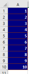
Example 1: Change the Interior Color of a Cell
Private Sub CommandButton1_Click()Range("A1:A10").Interior.Color = RGB(255, 0, 0)Range("B1:B10").Interior.ColorIndex = 49End Sub
One line uses RGB values to set part of column “A” to a background of red. The other uses ColorIndex to change it to a blue color. It looks like the image below when executed.

Example 2: Change the Font Color of a Cell
Private Sub CommandButton1_Click()Range("A1:A10").Font.Color = RGB(255, 0, 0)Range("B1:B10").Font.ColorIndex = 49End Sub
The first line changes the font in part of column A to a red color. The second line uses ColorIndex to change the font in part of column B to a dark blue color.

Example 3: Change the Border Color of a Cell
Private Sub CommandButton1_Click()Range("A1:A10").Borders.Color = RGB(255, 0, 0)Range("B1:B10").Borders.ColorIndex = 49Range("D1:D10").Borders(xlLeft).Color = RGB(0, 0, 255)Range("D1:D10").Borders(xlBottom).Color = RGB(255, 0, 255)Range("E1:E10").Borders(xlRight).ColorIndex = 4Range("E1:E10").Borders(xlTop).ColorIndex = 51End Sub
The first line changes all the borders of the A column range to RGB(255,0,0), which is red. The second line uses colorIndex to change all the borders in the B column range to a dark blue. Lines 4 through 8 show specific borders being colored.

Example 4: Background, Font, and Border Color Change
Private Sub CommandButton1_Click()Range("A1:A10").Interior.Color = RGB(0, 0, 128)Range("A1:A10").Font.Color = RGB(255, 255, 255)Range("A1:A10").Borders.ColorIndex = 53End Sub
Some Possible Colors Choices: Color Options
| Color | Index_ID | R | G | B |
| 1 | 0 | 0 | 0 | |
| 2 | 255 | 255 | 255 | |
| 3 | 255 | 0 | 0 | |
| 4 | 0 | 255 | 0 | |
| 5 | 0 | 0 | 255 | |
| 6 | 255 | 255 | 0 | |
| 7 | 255 | 0 | 255 | |
| 8 | 0 | 255 | 255 | |
| 9 | 128 | 0 | 0 | |
| 10 | 0 | 128 | 0 | |
| 11 | 0 | 0 | 128 | |
| 12 | 128 | 128 | 0 | |
| 13 | 128 | 0 | 128 | |
| 14 | 0 | 128 | 128 | |
| 15 | 192 | 192 | 192 | |
| 16 | 128 | 128 | 128 | |
| 17 | 153 | 153 | 255 | |
| 18 | 153 | 51 | 102 | |
| 19 | 255 | 255 | 204 | |
| 20 | 204 | 255 | 255 | |
| 21 | 102 | 0 | 102 | |
| 22 | 255 | 128 | 128 | |
| 23 | 0 | 102 | 204 | |
| 24 | 204 | 204 | 255 | |
| 25 | 0 | 0 | 128 | |
| 26 | 255 | 0 | 255 | |
| 27 | 255 | 255 | 0 | |
| 28 | 0 | 255 | 255 | |
| 29 | 128 | 0 | 128 | |
| 30 | 128 | 0 | 0 | |
| 31 | 0 | 128 | 128 | |
| 32 | 0 | 0 | 255 | |
| 33 | 0 | 204 | 255 | |
| 34 | 204 | 255 | 255 | |
| 35 | 204 | 255 | 204 | |
| 36 | 255 | 255 | 153 | |
| 37 | 153 | 204 | 255 | |
| 38 | 255 | 153 | 204 | |
| 39 | 204 | 153 | 255 | |
| 40 | 255 | 204 | 153 | |
| 41 | 51 | 102 | 255 | |
| 42 | 51 | 204 | 204 | |
| 43 | 153 | 204 | 0 | |
| 44 | 255 | 204 | 0 | |
| 45 | 255 | 153 | 0 | |
| 46 | 255 | 102 | 0 | |
| 47 | 102 | 102 | 153 | |
| 48 | 150 | 150 | 150 | |
| 49 | 0 | 51 | 102 | |
| 50 | 51 | 153 | 102 | |
| 51 | 0 | 51 | 0 | |
| 52 | 51 | 51 | 0 | |
| 53 | 153 | 51 | 0 | |
| 54 | 153 | 51 | 102 | |
| 55 | 51 | 51 | 153 | |
| 56 | 51 | 51 | 51 |
Excel VBA Resources
We can use conditional formatting to automatically change the cell background color based on the data value in the cell.
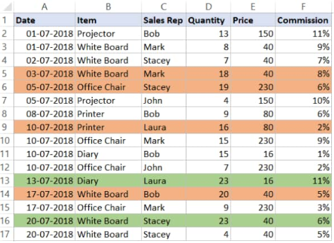 Figure 1. of Cell Color in Excel
Whenever we are dealing with large amounts of data in Excel, we can decide to pick out matching values and highlight them by using a specified color of font or cell background
How to Color Code in Excel
If we desire to change Excel color code based on the values in the cells, we must apply conditional formatting.
Since, we sometimes want to highlight an entire column (or row) instead of just a cell or two; this is why we will base the color code in Excel on matching values within the cells.
Let’s say we have the sales roaster containing the details of purchases made at a store during the year;
- We begin by collecting the data available to us in well labelled columns of our Excel worksheet:
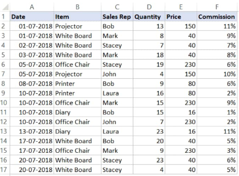 Figure 2. of Cell color in Excel
Our goal here is to highlight all the sales records for the Sales Rep named Bob.
- Select the whole dataset on our worksheet (A2:F17) and then click on the “Home” tab on the top left side of our worksheet:
 Figure 3. of Home Tab in Excel
- In the “Styles” group, open “Conditional Formatting”:
 Figure 4. of Conditional Formatting Tab in Excel
- Open ‘New Rule’:
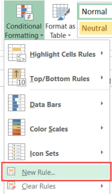 Figure 5. of New Conditional Formatting Rule in Excel
- A ‘New Formatting Rule’ fly out appears, click on the ‘Use formulas to determine which cells to format’ button:
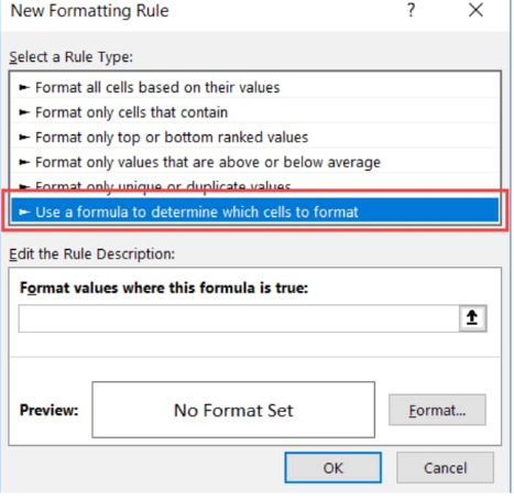 Figure 6. of New Formatting Rule in Excel
- In the formula dialogue box, input the following operation:
=$C2=”Bob”
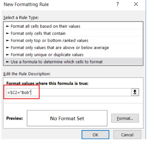 Figure 7. of New Formatting Rule in Excel
- Click on the ‘Format’ icon.
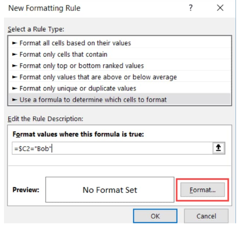 Figure 8. of New Formatting Rule in Excel
- In the next dialog box that emerges, we will set the Excel color which we want to use in highlighting the specified rows.
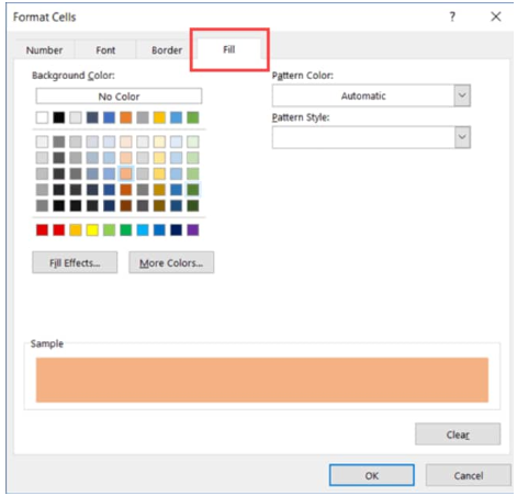 Figure 9. of Format Cell Color in Excel
- Clicking “OK” will highlight every row where Sales Rep “Bob” is located with the specified Excel color:
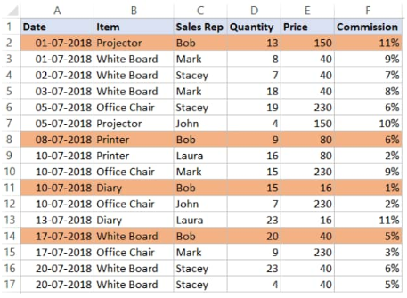 Figure 10. of Color Formatting in Excel
Conditional Formatting in Excel checks the data in every cell of our worksheet for the given condition, =$C2=”Bob”
So when it is analyzing the cells in row A2, Excel checks out the cell C2 for the name “Bob”. If it does, the cell becomes highlighted, otherwise it doesn’t.
Note
Be sure to use the dollar sign ($) in Excel before the column’s alphabet – $C1 – this will lock the column to remain as “C”; this way, when cell A2 gets checked by the formula, it also checks C2; similarly, when A3 gets checked for our criteria, it will also check C3.
This helps to ensure the entire row is highlighted by conditional formatting.