Color columns in excel - Word и Excel - помощь в работе с программами

Adding a color to alternate rows or columns (often called color banding) can make the data in your worksheet easier to scan. To format alternate rows or columns, you can quickly apply a preset table format. By using this method, alternate row or column shading is automatically applied when you add rows and columns.

Here’s how:

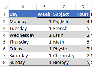
Select the range of cells that you want to format.
Click Home > Format as Table.
Pick a table style that has alternate row shading.
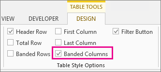
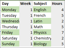
To change the shading from rows to columns, select the table, click Design, and then uncheck the Banded Rows box and check the Banded Columns box.

Tip: If you want to keep a banded table style without the table functionality, you can convert the table to a data range. Color banding won’t automatically continue as you add more rows or columns but you can copy alternate color formats to new rows by using Format Painter.

Use conditional formatting to apply banded rows or columns

You can also use a conditional formatting rule to apply different formatting to specific rows or columns.

Here’s how:

On the worksheet, do one of the following:
- To apply the shading to a specific range of cells, select the cells you want to format.
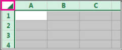
- To apply the shading to the whole worksheet, click the Select All button.
Click Home > Conditional Formatting > New Rule.
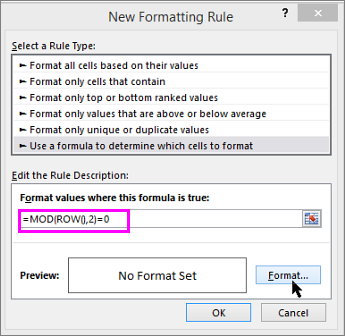
In the Select a Rule Type box, click Use a formula to determine which cells to format.
To apply color to alternate rows, in the Format values where this formula is true box, type the formula =MOD(ROW(),2)=0.

To apply color to alternate columns, type this formula: =MOD(COLUMN(),2)=0.

These formulas determine whether a row or column is even or odd numbered, and then applies the color accordingly.
Click Format.
In the Format Cells box, click Fill.
Pick a color and click OK.
You can preview your choice under Sample and click OK or pick another color.
Tips:
- To edit the conditional formatting rule, click one of the cells that has the rule applied, click Home > Conditional Formatting > Manage Rules > Edit Rule, and then make your changes.
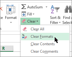
- To clear conditional formatting from cells, select them, click Home > Clear, and pick Clear Formats.
- To copy conditional formatting to other cells, click one of the cells that has the rule applied, click Home > Format Painter , and then click the cells you want to format.

Need more help?

Want more options?

Explore subscription benefits, browse training courses, learn how to secure your device, and more.

Communities help you ask and answer questions, give feedback, and hear from experts with rich knowledge.

Источник

Select the cell or range of cells you want to format. Click Home > Format Cells dialog launcher, or press Ctrl+Shift+F. On the Fill tab, under Background Color, pick the color you want. To use a pattern with two colors, pick a color in the Pattern Color box, and then pick a pattern in the Pattern Style box.

Contents

1 How do I fill a cell with color in Excel?
2 How do I change the color of a column in Excel based on value?
3 How do I automatically color code cells in Excel?
4 Is there a shortcut to fill color in Excel?
5 Can you use an IF statement to color a cell?
6 How do I change the color of a cell in Excel based on value in a cell?
7 How do I automatically color code?
8 What is the shortcut to highlight a column in Excel?
9 How do you highlight yellow in Excel?
10 How can I highlight in Excel?
11 How do I color text in Excel formula?
12 How do I change the highlight color in Excel?
13 How do I highlight all columns in Excel?
14 What does Alt u mean?
15 What is the shortcut key to highlight the entire columns?
16 Is there a fast way to highlight in Excel?
17 Where is the highlighter tool in Excel?
18 How do you highlight lines in Excel?

How do I fill a cell with color in Excel?

On the home tab, in the Styles subgroup, click on Conditional Formatting→New Rule. Now select Use a formula to determine which cells to format option, and in the box type the formula: D3>5; then select Format button to select green as the fill color.

How do I change the color of a column in Excel based on value?

On the Home tab, in the Styles group, click Conditional Formatting > New Rule… (see step 2 of How to dynamically change a cell color based on value for step-by-step guidance). In the “New Formatting Rule” dialog, select the option “Use a formula to determine which cells to format”.

How do I automatically color code cells in Excel?

You can color-code your formulas using Excel’s conditional formatting tool as follows. Select a single cell (such as cell A1). From the Home tab, select Conditional Formatting, New Rule, and in the resulting New Formatting Rule dialog box, select Use a formula to determine which cells to format.

Is there a shortcut to fill color in Excel?

The keyboard shortcut to open the Fill Color menu on the ribbon is Alt+H+H.Use the arrow keys on the keyboard to select the color you want. The arrow keys will move a small orange box around the selected color. Press the Enter key to apply the fill color to the selected cells.

Can you use an IF statement to color a cell?

Conditional formatting is applied using IF/THEN logical test only.For example, if you want to apply conditional formatting using a condition that “If a cell value is greater than a set value, say 100, then format the cell as RED, else format the cell as GREEN”.

How do I change the color of a cell in Excel based on value in a cell?

3 Answers

Select cell B3 and click the Conditional Formatting button in the ribbon and choose “New Rule”.
Select “Use a formula to determine which cells to format”
Enter the formula: =IF(B2=”X”,IF(B3=”Y”, TRUE, FALSE),FALSE) , and choose to fill green when this is true.

How do I automatically color code?

Here’s how to do it:

Select the desired data range.
Go to Data -> Sort & Filter -> Sort.
Select the desired column in your data range.
For the Sort on option, select Cell Color.
Choose a color in the Order.
Select On Top in the final drop-down list.
Hit OK.

What is the shortcut to highlight a column in Excel?

Let’s see how easy is selecting columns in excel. Select any cell in any column. Press Ctrl + Space shortcut keys on the keyboard. The whole column will be highlighted in excel to show the selected column, as shown below in the picture.

How do you highlight yellow in Excel?

Create a cell style to highlight cells
Click Format. In the Format Cells dialog box, on the Fill tab, select the color that you want to use for the highlight, and then click OK. Click OK to close the Style dialog box. The new style will be added under Custom in the cell styles box.

How can I highlight in Excel?

How to Highlight Cells in Excel

Open the Microsoft Excel document on your device.
Select a cell you want to highlight.
From the top menu, select Home, followed by Cell Styles.
A menu with a variety of cell color options pops up.
When you find a highlight color that you like, select it to apply the change.

How do I color text in Excel formula?

Apply conditional formatting based on text in a cell

Select the cells you want to apply conditional formatting to. Click the first cell in the range, and then drag to the last cell.
Click HOME > Conditional Formatting > Highlight Cells Rules > Text that Contains.
Select the color format for the text, and click OK.

How do I change the highlight color in Excel?

Under Personal, click Appearance. On the Highlight color pop-up menu, click the color that you want. Note: You must close and then reopen Excel to see the new highlight color.

How do I highlight all columns in Excel?

Excel Tips: Select an Entire Row or Column

To select an entire row, click the row number or press Shift+spacebar on your keyboard.
To select an entire column, click the column letter or press Ctrl+spacebar.
To select multiple rows or columns, click and drag over several row numbers or column letters.

What does Alt u mean?

Alt+U is a keyboard shortcut most often used to change text to uppercase.Computer keyboard shortcuts.

What is the shortcut key to highlight the entire columns?

Ctrl+Space is the keyboard shortcut to select an entire column.

Is there a fast way to highlight in Excel?

Lets examine both: The first one is CTRL + ARROW KEYS. This will allow you to quickly jump around your spreadsheet by moving your cursor to the next available Excel Cell of your next data range.

Where is the highlighter tool in Excel?

You find Excel’s highlight function under the “Conditional Formatting” button in the Styles section under the Home tab. When you click it, a drop-down menu appears with a “Highlight Cell Rules” option.

How do you highlight lines in Excel?

Press and hold down the “Ctrl” key on the keyboard. Click the second line number. Both rows now appear highlighted, but this will change as soon as you click off them.

Источник

Download PC Repair Tool to quickly find & fix Windows errors automatically

If you want to apply color in alternate rows and columns in an Excel spreadsheet, here is what you need to do. It is possible to show the desired color in every alternate row or column with the Conditional Formatting. This functionality is included in Microsoft Excel, and you can make use of it with the help of this tutorial.

Let’s assume that you are making a spreadsheet for your school or office project, and you have to colorize every alternate row or column. There are two ways to do that in Microsoft Excel. First, you can select particular rows or columns and change the background color manually. Second, you can use the Conditional Formatting functionality to apply the same in automation. Either way, the result will be the same, but the second method is more efficient and time saving for any user.

How to alternate row colors in Excel

To apply color in alternate rows or columns in Excel, follow these steps-

Open the spreadsheet with Excel.
Select the rows and columns that you want to colorize.
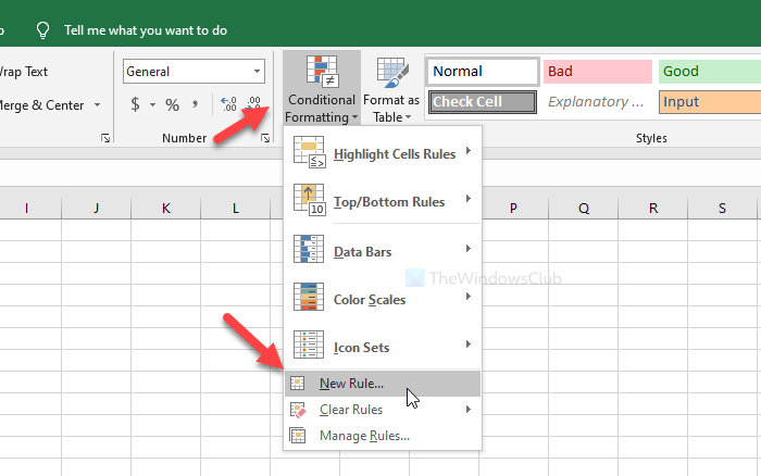
Click the Conditional Formatting in the Home tab.
Select New Rule from the list.
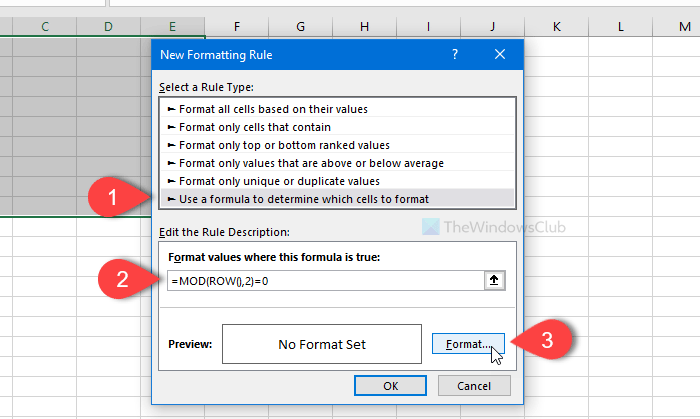
Select Use a formula to determine which cells to format.
Enter =MOD(ROW(),2)=0 or =MOD(COLUMN(),2)=0 in the Format values box.
Click the Format button.
Switch to the Fill tab.
Select a color that you want to use.
Click the OK button twice.

Let’s check out these steps in detail.

At first, open the spreadsheet with Excel. In case, you do not have the spreadsheet, create it first so that you can understand whether you want to colorize the rows or columns. Once done, use your mouse to select all the cells (rows and columns). If you’re going to apply the color scheme to the entire spreadsheet, click the arrow icon that allows you to select the spreadsheet from top to bottom.

Now make sure that you are in the Home tab. If so, click on the Conditional Formatting in the Styles section, and select the New Rule option from the list.

Following that, select the Use a formula to determine which cells to format option, and write down one of these in the Format values box-

=MOD(ROW(),2)=0
=MOD(COLUMN(),2)=0

The first one will colorize the desired color in alternate rows and the second one is for columns. After that, click the Format button.

Now, switch to the Fill tab, select a color that you want to use, and click on the OK button.

Then, you will have to click the OK button again to apply the change.

How to apply shading to alternate rows and columns in Excel?

In order to apply shading to alternative rows and columns in Excel, you need to use Conditional Formatting. It is required to use this function: =MOD(ROW(),2)=0 or =MOD(COLUMN(),2)=0. Then, you can switch to the Format menu and Fill tab to choose the color as per your requirements.

How to set color to alternate rows and columns in Excel?

As said earlier, you need to use a function to set colors to alternative rows and columns. First, you need to open the Conditional Formatting section and set a new rule. Then, select the Use a formula to determine which cells to format and use this formula: =MOD(ROW(),2)=0 or =MOD(COLUMN(),2)=0. Next, you can fill the rows and columns with your desired color.

That’s all! Now you can see the selected color in every alternate row or column.

Ezoic

When he is not writing about Microsoft Windows or Office, Sudip likes to work with Photoshop. He has managed the front end and back end of many websites over the years. He is currently pursuing his Bachelor’s degree.

Источник

You must have seen some Excel spreadsheets with alternating colors in rows or columns. It can make the data more vibrant and easy to distinguish. Here I’ll introduce 2 commonly used methods to make a table like this.

How to Shade Every Other Row in Excel with Conditional Formatting

1. First, select the range of cells you want to shade.

2. Switch to Home tab, click Conditional Formatting and choose New Rule… in the drop-down list.

3. Select Use a formula to determine which cells to format as the rule type.

4. Enter the formula “=mod(row(),2)=0” in the textbox below Format values where this formula is true. Then click Format… on the lower right corner.

5. Choose a Background Color in Fill tab. Click OK to confirm it.

6. Hit OK again in New Formatting Rule window to implement the rule.

Now the rows of even number are shaded with blue. If you want to also apply colors to the rows of odd number, you can shade all the selected cells with a color at first and then follow above steps to apply another color to every other row.

Or you can repeat the steps to add a new rule but change the formula into “=mod(row(),2)=1”

The color of odd number rows can be changed in this way as well.

You can shade every other column in the similar way. Just change the formula a little bit to “=mod(column(),2)=0” and “=mod(column(),2)=1”

How to Apply Color to Alternate Rows and Columns with Table Style

If you are not good at remembering formula, try this method.

1. Select all the cells you want to shade.

2. Switch to Home tab and click Format as Table in Style section to open the drop-down menu and choose a template you like.

3. Then choose a range of cells as the table area. Check or uncheck My table has headers according to your actual situation.

4. You can also adjust the color and apply some options to the table in the Table Tools of Design tab.

But if you want to apply colors to alternating rows or columns more freely, you’d better try the first method using Conditional Formatting.

Copyright Statement: Regarding all of the posts by this website, any copy or use shall get the written permission or authorization from Myofficetricks.

Источник

Tables are often used to layout and summarize data. But have you been in a situation where the table got so big that it is not easy to read? The table is so big that it is hard to tell which rows and columns a certain cells belong. For example, in the table below, it is hard to tell which row the “Y”‘s are starting from the 3rd row.

The Excel file with the examples used in this post: Conditional Formatting

As a table gets bigger, it is easier to confuse which row or column each cell belongs to. Alternating bands of colors can make a table more intuitive and easy to read. The “Y”‘s closer to the middle is especially hard to tell which row it belongs to.

To make things more intuitive, you can use alternate shades on each row or column on the table using conditional formatting.

Below is a formula that returns true for each odd row.

=MOD(ROW(),2)=1

The conditional formatting rule shades the background of each odd row, leaving the even rows with no color. And gets something like this:

Alternate Column Colors

The same thing could be done for columns. The following line returns true for all odd columns

=MOD(COLUMN(),2)=1

In this example, data is laid out in a long table, making the 3 to 7’s hard to read. The alternating column colors make reading the table much more intuitive.

When a table has many rows, it’s hard to figure out which column the data is in, especially ones in the middle of the table.

Coloring every other column makes the table much more intuitive to read.

For a long table with a lot of columns, always make it easier for the reader by using conditional formatting on the columns.

Checker Patterns

A checker pattern is a combination of alternating row and column colors, with a white cell for “intersecting” cells. Below is the conditional formatting rules window used to make the checker pattern. Note the order, the white cell format must go first:

Formulas for each corresponding conditional formatting rule:

=MOD(ROW(),2)=0,MOD(COLUMN(),2)=0)  <- selects the intersecting cell
=MOD(ROW(),2)=1  <- selects odd row
=MOD(COLUMN(),2)=1 <- selects odd columns

Instead of shading the intersecting cell white, a 3rd color can be used instead. In this case, blue.

2 people found this article useful

Источник