
Содержание
- How to Automatically Color Code in Excel
- The Big Picture
- Basic Color Coding Options
- Highlight Duplicates
- Sort by Color
- Highlight Top 10
- Advanced Options
- Show Variances with Data Bars
- Highlight Positive, Neutral, and Negative Values with Icon Sets
- Show Variances with Color Scales
- Smooth and Easy
- How to Enter Your Custom Color Codes in Microsoft Excel
- Step 1: Make Your Chart
- Step 2: Edit Your Chart as Needed
- Step 3: Select Your Chart
- Step 4: Click on More Fill Colors
- Step 5: Choose a Custom Fill
- Step 6: Type Your RGB Codes
- Bonus
- 7 Comments
- How to Color Code in Excel for Financial Models (PC/Windows Version) [Tutorial Video] (32:42)
- How to Color Code in Excel: Key PC and Mac Shortcuts
- How to Color Code in Excel: What Financial Models Should Look Like
- Other Principles of Financial Model Formatting
- How to Automate the Color-Coding Process in Excel
How to Automatically Color Code in Excel

MS Excel is one of the most powerful and versatile programs in the MS Office bundle. Unless you work with spreadsheets, you probably don’t even use this program, but it is important to realize just how tweakable and programmable it really is. For instance, you could program the Monopoly boardgame using nothing but Excel. Color coding, however, is much easier to use in this great spreadsheet program.
Conditional formatting gives you the ability to automize cell formatting in accordance with the inserted value in MS Excel. The most popular type of conditional formatting in Excel is automatic color coding.
This is very useful for presentation and visualization, but also in instances where creating gradually changing shades (depending on the cell value) is essential in capturing the big picture of a spreadsheet. The best example of this is sorting temperature values by months.
The Big Picture
Jumping right into color coding is certainly a possibility, but, in truth, conditional formatting takes planning before anything else. During the planning process, whenever you come up with a color-coding idea, ask yourself: “Does this make my life simpler or more complicated?” Technically, you could “tell” Excel to color every cell that contains an irrational number red. This is not necessarily a bad idea, but if you also plan to color code it to change shade intensity as the numbers grow, it may end up confusing.
On the other hand, if you’re creating a spreadsheet for a maths class, wanting your irrational number cells to be colored red is a perfectly imaginable and a viable idea. The point is, you shouldn’t jump straight into color coding without actually thinking about how you’re going to make the entire spreadsheet picture become the best it can be. This takes time and a lot of trial and error.

Basic Color Coding Options
There are a number of options that can help you in your color coding task and knowing how each one works will make your job easier.
Highlight Duplicates
This is one of the most basic color coding tasks that you give Excel. What it essentially does, is it marks all the duplicate names in the same color. This may help you remove the duplicate names, or may assist you in further spreadsheet analysis. Here’s how to highlight duplicates.

- First, you’ll need to select the range of cells that you want to check for duplicates. Of course, by pressing Ctrl + A, you’ll select every cell in the table.

- Go to the Home tab and navigate to Conditional Formatting.
- Under Conditional Formatting, go to Highlight Cell Rules, and then to Duplicate Values.
- The Window that pops up offers you to select the format from two drop-down lists.
- The first drop-down list allows you to choose which cells you want colored, Duplicate ones or the Unique
- The second drop-down list offers you a set of available colors.
- Press OK.


Sort by Color
Sorting your list by color takes you a step further from duplicate highlighting. If you’ve highlighted the duplicates, the sort by color option will allow you to sort them together, which works fantastically with larger lists. Here’s how to do it:
- Select the desired data range.
- Go to Data ->Sort & Filter ->Sort.
- Select the desired column in your data range.
- For the Sort on option, select Cell Color.
- Choose a color in the Order
- Select On Top in the final drop-down list.
- Hit OK.

This will sort your list and put the duplicates at the top.
Highlight Top 10
Whether we’re talking about geography, finances, or temperatures, the top 10 items on a list tend to tell a good part of the list’s story. Of course, using the same principle below, you can highlight the bottom 10, top 10%, bottom 10%, above average, below average, and many other data groups.
- Select the desired data range
- Go to the Home
- Click Conditional Formatting.
- Go to Top/Bottom Rules.
- Select Top 10 Items.
- In the window that pops up, adjust the number of options you want (you can do more and less than 10, of course).
- Now select the fill color.
- Hit OK.

Advanced Options
These were some basic color coding options that Excel offers. Now, let’s go over the more advanced tasks. Don’t worry, they aren’t any more complicated than the previous three.
Show Variances with Data Bars
Data bars essentially draws a bar in each cell, with the length corresponding to the cell value of other cells. Here’s a picture to explain it.

Here’s how to select the column/range that you want to format.
- Select the desired data range
- Go to the Home
- Navigate to Conditional Formatting ->Data Bars.
- Select the desired color and fill style.

Highlight Positive, Neutral, and Negative Values with Icon Sets
This will show you how to custom set the positive, neutral, and negative values next to items. This is very useful for sales and revenue breakdowns.
- Select the column/range that you want to format.
- Go to the Home
- Navigate to Conditional Formatting ->Icon Sets.
- Choose the icon style that you want to use.
- Excel will automatically interpret your data.
- If you want to change it, go to Manage Rules under Conditional Formatting.
- Choose the Icon Set rule and click Edit Rule.
- Adjust the rules according to your preferences.


Show Variances with Color Scales
Using the Color Scales under Conditional Formatting works pretty much the same way as the Icon Sets, only displays the result differently and with more gradients.
- Select the range.
- Find Color Scales in Conditional Formatting.
- Choose the color scale.

Smooth and Easy
Conditional formatting is pretty much basic formatting with some rule setting. Nevertheless, it is very useful and brings out Excel’s true nature – it’s more than a tool for table formatting, its an ultimate program for creating spreadsheets.
What interesting tips do you have to share about Excel? People who work with spreadsheets tend to have their own processes. How does your work? Hit the comment section below with any advice, tips, and questions.
Источник
How to Enter Your Custom Color Codes in Microsoft Excel

If you want to look polished, then you have no other choice but to customize your visualization’s color palette. Don’t worry–customizing your colors is an easy low-hanging-fruit edit. Locate your style guide, scroll down to the color section, and decode the jargon. If you don’t have a style guide, or can’t find it, identify your color codes with an eyedropper or with Paint.
Then, enter your color codes in Excel!
Step 1: Make Your Chart
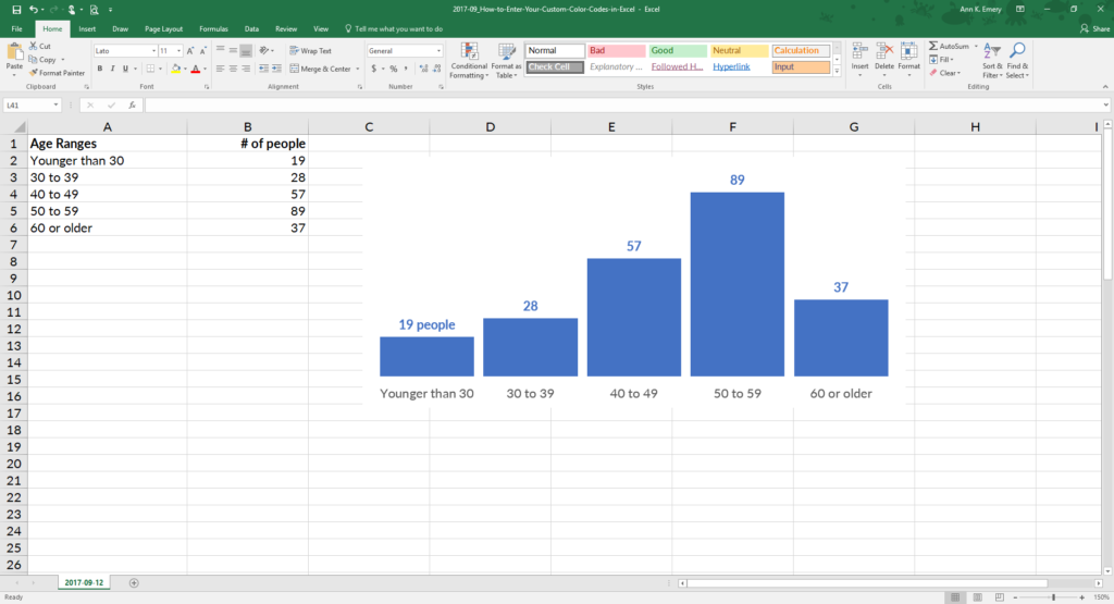
Build your graph. Here’s a histogram that displays how many people fell into each age range. The default graph has Microsoft’s blue.

Step 2: Edit Your Chart as Needed
Declutter that cluttered graph. Delete the border, grid lines, title, and vertical axis. Label the columns directly. Nudge the columns closer together.
Step 3: Select Your Chart
Now it’s time to customize the color. Click on the bar, line, or pie wedge that you want to adjust. Can you see that the columns are selected?

Step 4: Click on More Fill Colors
Go to Chart Tools, then Format, and then Shape Outline (line graphs) or Shape Fill (all other types of graphs, like this one). Ignore the default colors! Go to the bottom where it says More Fill Colors.

Step 5: Choose a Custom Fill
On the pop-up window, click on the Custom tab.

Step 6: Type Your RGB Codes
Enter your RGB code. RGB stands for red, green, and blue. This is the recipe of reds, greens, and blues that get mixed together to produce your exact shade.
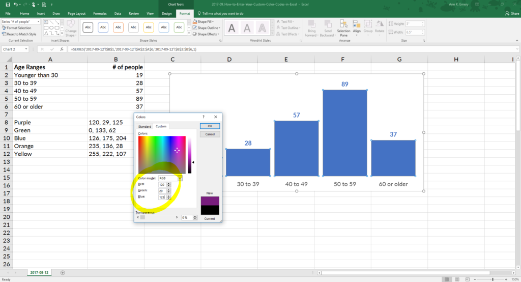
I used 120, 29, 125, which is the exact shade of purple from a client’s logo. Now I can quickly customize other pieces of the graph, like the numeric labels, because that purple is already stored under Recent Colors.

Bonus
With just a few clicks, custom colors reinforce branding and make you look professional.
I love doing this, but every time I turn off my computer, the RGB codes go away. I’ve become pretty good at memorizing them, but is there a way to save the RGB codes somewhere in Word or Excel so I can reuse them? Right now I keep track of them in Evernote.
Yes! Go to Page Layout –> Colors –> Customize Colors.
You just made my life soooo much easier – thank you!
I prefer to use Custom Colors as it always make the data much presentable. This is a good piece of info.
[…] locate your color codes with an eyedropper, or locate your color codes with Microsoft Paint. Then, enter your color codes in Excel or in […]
I’m using Excel version 2019 Volume 16.59 and cannot find the customize color feature. Was this added in later versions? And if so is there a work around so i can create a custom color palette?
Thank you
Are you using a Mac by any chance? If so, go into PowerPoint and try it there. Let me know if that works. Otherwise, we can keep troubleshooting. — Ann
Источник
How to Color Code in Excel for Financial Models (PC/Windows Version) [Tutorial Video] (32:42)
In this lesson, you’ll learn how to apply color coding and formatting to financial models and fix problems with decimals, currency signs, indentation, alignment, links vs. formulas vs. constants, and more – and you’ll practice by fixing the formatting on the Summary spreadsheet.
- Tutorial Summary
- Files & Resources
- Premium Course
This sample lesson from our Excel/VBA course covers how to color code in Excel and some of the key principles for formatting financial models.
Table of Contents:
1:06: Formatting Principles
11:02: Demonstration of Walmart Model Fixes
19:59: Exercise – Summary Spreadsheet Fixes
30:34: Recap and Summary
We have some general guidelines for model formatting, but these are not like the laws of physics (gravity, momentum, speed of light, etc.) – they’re “rules of thumb” rather than “laws of nature.”
How to Color Code in Excel: Key PC and Mac Shortcuts
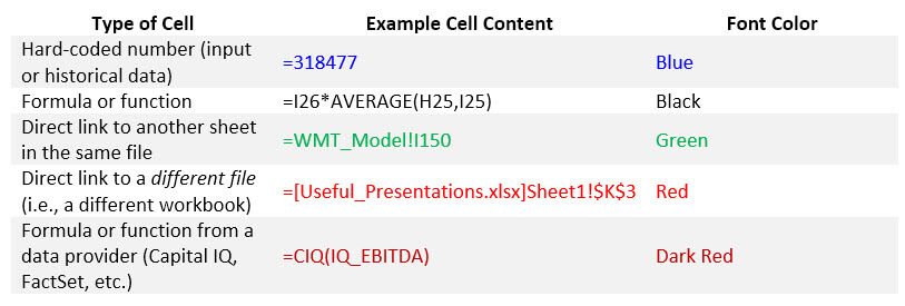
We use the following colors for different types of cells:
To find and select these cells, you can use the following PC/Windows shortcuts:
F5: Jump to Cell
F5, Alt + S, O, X: Select Constants (Drop the X if you want to highlight text constants)
F5, Alt + S, F, X: Select Formulas (Drop the X to highlight textual formulas)
Ctrl + 1: Format Dialog Box
Ctrl + F: Find
For example, if you press F5, Alt + S, O, X, that will highlight all constants on the spreadsheet. You can then press Ctrl + 1 to change their font color to blue, or you can access the font color commands from the “Home” tab in the ribbon menu.
To find direct links to other spreadsheets in the file, you can press Ctrl + F and search for the “!” character, which always indicates links to other sheets.
To find links to other files, search for “.xls” using Ctrl + F, and change the font color to red for each instance.
In the Mac version of Excel, you can use these shortcuts instead:
F5 or Ctrl + G: Jump to Cell
F5 or Ctrl + G, Special, Constants: Select Constants (Drop the X if you want to highlight text constants)
F5 or Ctrl + G, Special, Formulas: Select Formulas (Drop the X to highlight textual formulas)
⌘ + 1: Format Dialog Box
⌘ + F: Find
How to Color Code in Excel: What Financial Models Should Look Like
If you follow these standards for color coding, your financial models should look like the examples below.
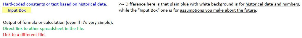
Here’s the normal color-coding scheme:
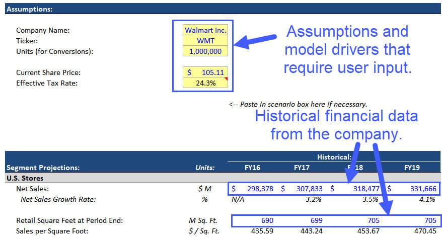
We use a yellow background and grey border for “input cells” that are assumptions or drivers in the model, while we use a white background with no borders for historical financial data:
Here are a few other examples of cell colors based on their categories and contents:
Other Principles of Financial Model Formatting
In addition to the points above about color-coding, we follow these guidelines with other types of formatting:
Centering: We use the “Accounting” format and variations of the “Percentage” format for most numbers, so centering is not an issue there. For the input boxes, we prefer to center percentages, dates, text, and normal numbers, but we do not apply it to anything in the “Accounting” format.
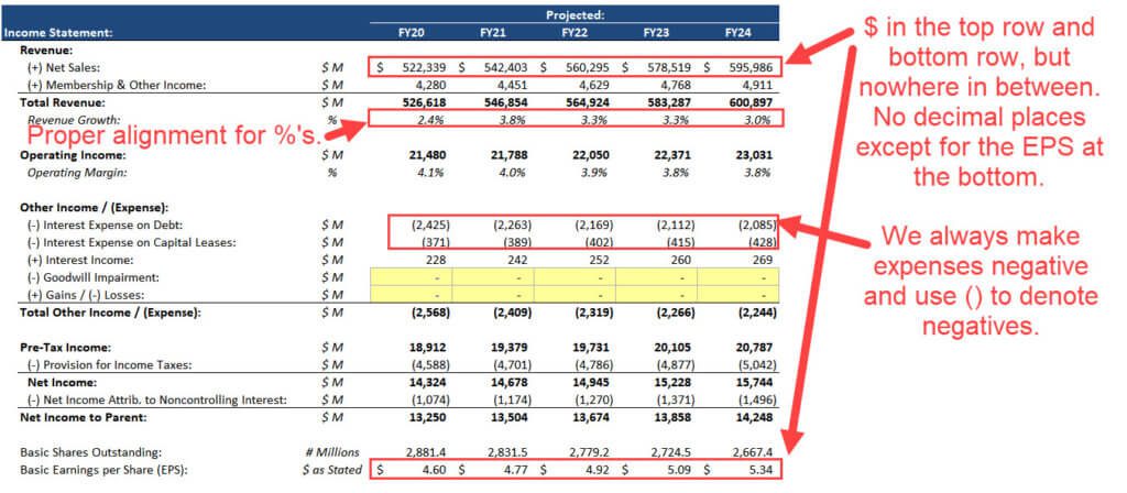
Dollar or Other Currency Signs: Only display these in the top row and bottom row of schedules. Sometimes it’s a bit ambiguous what a “schedule” is – often, we’ll display these in the top and bottom rows of each major segment.
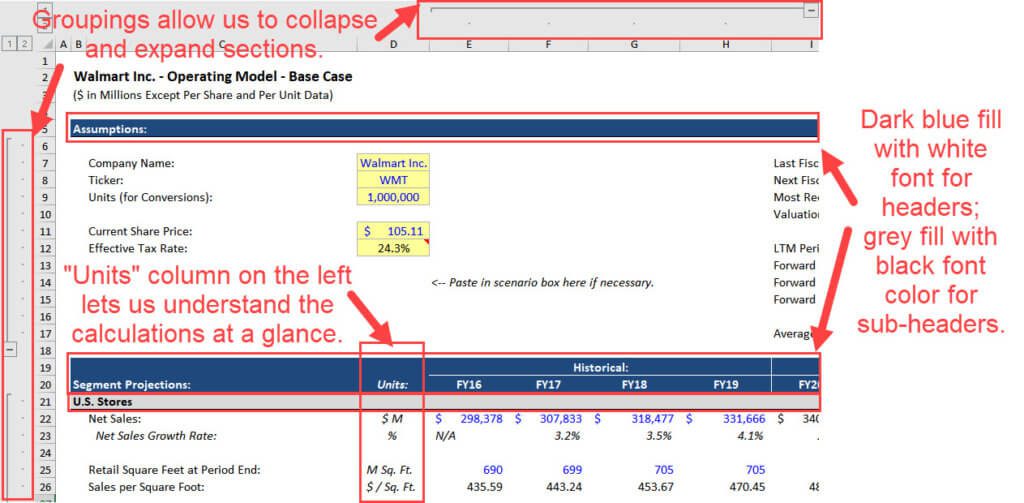
“Units”: We like to use an extra column to display the units, especially in schedules that mix $ per Sq Ft and Sq Ft and other figures with actual $, to remove ambiguity.
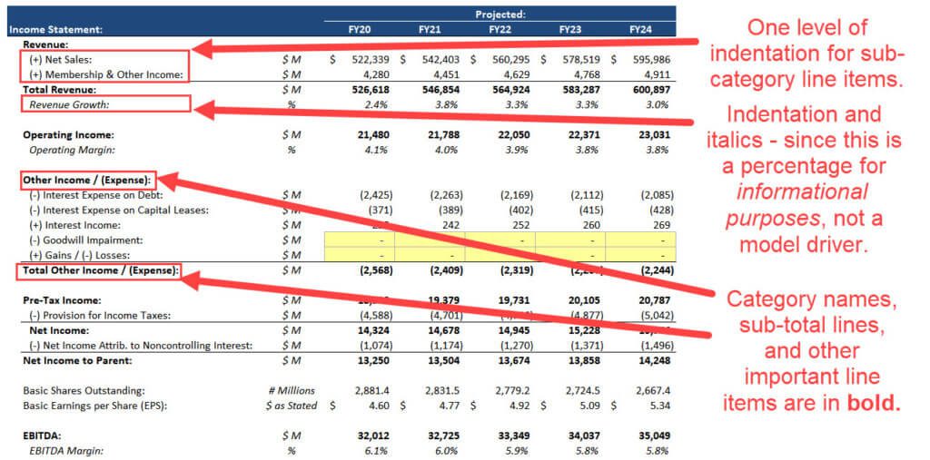
Indentation: We indent the individual rows within each category, and we use multiple indents for sub-categories. We also indent percentages used for informational purposes such as the margin formulas.
Signs: On the IS and CFS, we often use (+) and (-) when it is meaningful to do so – for example, if everything in a row is going to be positive or negative, and it’s easy to specify which is which.
Italics: We usually italicize percentages used for informational purposes – so, the overall margins and revenue growth rates, but not the assumptions used to calculate them in the first place. Those are in the yellow input boxes!
Decimals: It doesn’t matter what you do as long as you’re consistent. Use 1 decimal, 0 decimals, or 2 decimal places for all the financial figures in your model… exceptions apply for the Share Price and EPS figures, which almost always use 2 decimal places because of how share prices are displayed.
We also usually use at least 1 decimal place, sometimes up to 2-3, to display the company’s share count. Usually 1 decimal place for valuation multiples and percentages as well – even if the financial figures in the model have 0 decimal places, as is the case here.
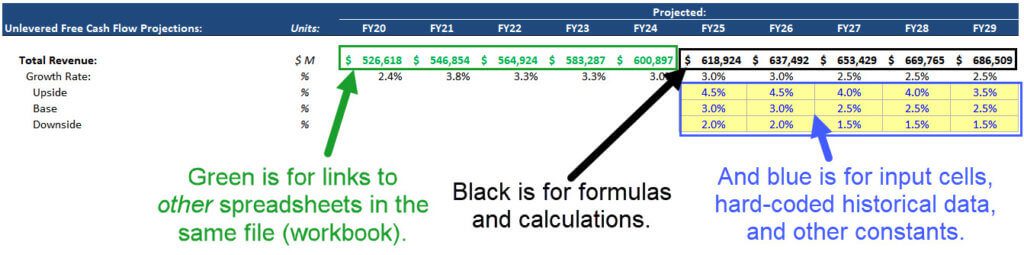
Headers: We use a blue background color, white text, and the “FY” format for the top header with the Historical and Projected years. We then use a grey background color for the other headers in a schedule – sometimes display the years on top depending on the spacing.
You can view examples of these standards in action below:
How to Automate the Color-Coding Process in Excel
It’s difficult to automate “all” this formatting, but you can automate much of the color-coding process if you feel comfortable using VBA, which we cover in the final module of this course.
In short, you can use the .SpecialCells, Union, and Intersect commands to find the appropriate cells, loop through them, and change the colors appropriately.
You can get the full Excel file (.xlsm) or just the .xlam file for the VBA code itself below:
Note: You must know Excel fairly well to use macros. If not, you could do serious damage to your spreadsheets. If you have little experience in Excel, then you should not mess around with this macro.
Источник
This sample lesson from our Excel/VBA course covers how to color code in Excel and some of the key principles for formatting financial models.
Table of Contents:
1:06: Formatting Principles
11:02: Demonstration of Walmart Model Fixes
19:59: Exercise – Summary Spreadsheet Fixes
30:34: Recap and Summary
We have some general guidelines for model formatting, but these are not like the laws of physics (gravity, momentum, speed of light, etc.) – they’re “rules of thumb” rather than “laws of nature.”
How to Color Code in Excel: Key PC and Mac Shortcuts
We use the following colors for different types of cells:
To find and select these cells, you can use the following PC/Windows shortcuts:
F5: Jump to Cell
F5, Alt + S, O, X: Select Constants (Drop the X if you want to highlight text constants)
F5, Alt + S, F, X: Select Formulas (Drop the X to highlight textual formulas)
Ctrl + 1: Format Dialog Box
Ctrl + F: Find
For example, if you press F5, Alt + S, O, X, that will highlight all constants on the spreadsheet. You can then press Ctrl + 1 to change their font color to blue, or you can access the font color commands from the “Home” tab in the ribbon menu.
To find direct links to other spreadsheets in the file, you can press Ctrl + F and search for the “!” character, which always indicates links to other sheets.
To find links to other files, search for “.xls” using Ctrl + F, and change the font color to red for each instance.
In the Mac version of Excel, you can use these shortcuts instead:
F5 or Ctrl + G: Jump to Cell
F5 or Ctrl + G, Special, Constants: Select Constants (Drop the X if you want to highlight text constants)
F5 or Ctrl + G, Special, Formulas: Select Formulas (Drop the X to highlight textual formulas)
⌘ + 1: Format Dialog Box
⌘ + F: Find
How to Color Code in Excel: What Financial Models Should Look Like
If you follow these standards for color coding, your financial models should look like the examples below.
Here’s the normal color-coding scheme:
We use a yellow background and grey border for “input cells” that are assumptions or drivers in the model, while we use a white background with no borders for historical financial data:
Here are a few other examples of cell colors based on their categories and contents:
Other Principles of Financial Model Formatting
In addition to the points above about color-coding, we follow these guidelines with other types of formatting:
Centering: We use the “Accounting” format and variations of the “Percentage” format for most numbers, so centering is not an issue there. For the input boxes, we prefer to center percentages, dates, text, and normal numbers, but we do not apply it to anything in the “Accounting” format.
Dollar or Other Currency Signs: Only display these in the top row and bottom row of schedules. Sometimes it’s a bit ambiguous what a “schedule” is – often, we’ll display these in the top and bottom rows of each major segment.
“Units”: We like to use an extra column to display the units, especially in schedules that mix $ per Sq Ft and Sq Ft and other figures with actual $, to remove ambiguity.
Indentation: We indent the individual rows within each category, and we use multiple indents for sub-categories. We also indent percentages used for informational purposes such as the margin formulas.
Signs: On the IS and CFS, we often use (+) and (-) when it is meaningful to do so – for example, if everything in a row is going to be positive or negative, and it’s easy to specify which is which.
Italics: We usually italicize percentages used for informational purposes – so, the overall margins and revenue growth rates, but not the assumptions used to calculate them in the first place. Those are in the yellow input boxes!
Decimals: It doesn’t matter what you do as long as you’re consistent. Use 1 decimal, 0 decimals, or 2 decimal places for all the financial figures in your model… exceptions apply for the Share Price and EPS figures, which almost always use 2 decimal places because of how share prices are displayed.
We also usually use at least 1 decimal place, sometimes up to 2-3, to display the company’s share count. Usually 1 decimal place for valuation multiples and percentages as well – even if the financial figures in the model have 0 decimal places, as is the case here.
Headers: We use a blue background color, white text, and the “FY” format for the top header with the Historical and Projected years. We then use a grey background color for the other headers in a schedule – sometimes display the years on top depending on the spacing.
You can view examples of these standards in action below:
How to Automate the Color-Coding Process in Excel
It’s difficult to automate “all” this formatting, but you can automate much of the color-coding process if you feel comfortable using VBA, which we cover in the final module of this course.
In short, you can use the .SpecialCells, Union, and Intersect commands to find the appropriate cells, loop through them, and change the colors appropriately.
You can get the full Excel file (.xlsm) or just the .xlam file for the VBA code itself below:
Full Excel File with Color-Code Macro
Color-Code Macro VBA Code
Note: You must know Excel fairly well to use macros. If not, you could do serious damage to your spreadsheets. If you have little experience in Excel, then you should not mess around with this macro.
Combined shape 37
Created with Sketch.
Based on the content of this tutorial, our recommended Premium Course Upgrade is…
Other BIWS Courses Include:
Polygon 1
Created with Sketch.
BIWS Premium:
Get the Excel & VBA, Financial Modeling Mastery, and PowerPoint Pro courses together and learn everything from Excel shortcuts up through advanced modeling, VBA to automate your workflow, and PowerPoint and presentation skills.
Learn More
Polygon 1
Created with Sketch.
BIWS Platinum:
The most comprehensive package on the market today for investment banking, private equity, hedge funds, and other finance roles. Includes ALL the courses on the site, plus updates and any new courses in the future.
Learn More
We can use conditional formatting to automatically change the cell background color based on the data value in the cell.
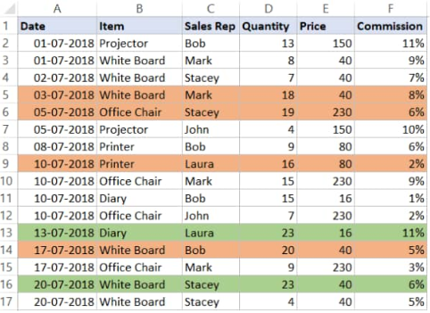 Figure 1. of Cell Color in Excel
Whenever we are dealing with large amounts of data in Excel, we can decide to pick out matching values and highlight them by using a specified color of font or cell background
How to Color Code in Excel
If we desire to change Excel color code based on the values in the cells, we must apply conditional formatting.
Since, we sometimes want to highlight an entire column (or row) instead of just a cell or two; this is why we will base the color code in Excel on matching values within the cells.
Let’s say we have the sales roaster containing the details of purchases made at a store during the year;
- We begin by collecting the data available to us in well labelled columns of our Excel worksheet:
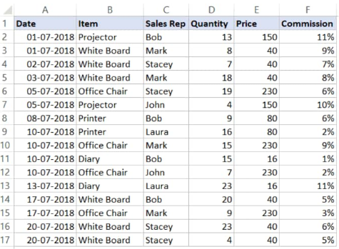 Figure 2. of Cell color in Excel
Our goal here is to highlight all the sales records for the Sales Rep named Bob.
- Select the whole dataset on our worksheet (A2:F17) and then click on the “Home” tab on the top left side of our worksheet:
 Figure 3. of Home Tab in Excel
- In the “Styles” group, open “Conditional Formatting”:
 Figure 4. of Conditional Formatting Tab in Excel
- Open ‘New Rule’:
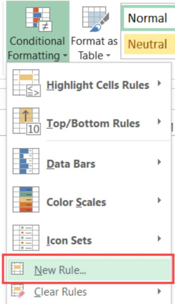 Figure 5. of New Conditional Formatting Rule in Excel
- A ‘New Formatting Rule’ fly out appears, click on the ‘Use formulas to determine which cells to format’ button:
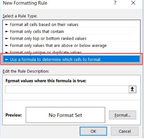 Figure 6. of New Formatting Rule in Excel
- In the formula dialogue box, input the following operation:
=$C2=”Bob”
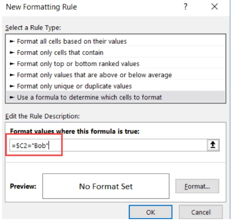 Figure 7. of New Formatting Rule in Excel
- Click on the ‘Format’ icon.
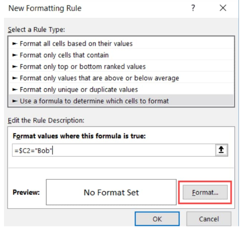 Figure 8. of New Formatting Rule in Excel
- In the next dialog box that emerges, we will set the Excel color which we want to use in highlighting the specified rows.
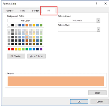 Figure 9. of Format Cell Color in Excel
- Clicking “OK” will highlight every row where Sales Rep “Bob” is located with the specified Excel color:
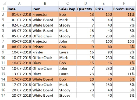 Figure 10. of Color Formatting in Excel
Conditional Formatting in Excel checks the data in every cell of our worksheet for the given condition, =$C2=”Bob”
So when it is analyzing the cells in row A2, Excel checks out the cell C2 for the name “Bob”. If it does, the cell becomes highlighted, otherwise it doesn’t.
Note
Be sure to use the dollar sign ($) in Excel before the column’s alphabet – $C1 – this will lock the column to remain as “C”; this way, when cell A2 gets checked by the formula, it also checks C2; similarly, when A3 gets checked for our criteria, it will also check C3.
This helps to ensure the entire row is highlighted by conditional formatting.
Conditional Formatting in Excel is very useful to highlight cells based on cell value. In this easy tutorial, learn the basics of how to do so.
![]()
Contents
- 1. Introduction
- 2. The Final Result
- 3. The Plain Spreadsheet
- 4. Use SUMIF for Summary
- 5. Applying Conditional Formatting
- 6. Less-Than-or-Equal-To condition
- Summary
- See Also
1. Introduction
Color coding of cells based on a condition is very useful in Excel for highlighting areas and data points. It is one of the top tools in the arsenal of an Excel expert in making the spreadsheet look snazzy and convey crucial information. In this article, we show a simple example of how to apply conditional formatting to cells based on values.
2. The Final Result
The sample spreadsheet we are using is the monthly sales figures and shown for each month. The screenshot below shows the cells highlighted in different colors depending on the threshold specified. Let us see how we can achieve this starting from a plain sheet.

3. The Plain Spreadsheet
Here is how the spreadsheet looks without any formatting applied. And without the threshold and summarizing cells too.

4. Use SUMIF for Summary
Let us enter a couple of summarizing cells using the SUMIF formula so we can verify the results. We use SUMIF to compute the total of sales figures which exceed the threshold (of $600). The formula for the cell labelled Sum of Greater is shown below.
=SUMIF(B2:B13,"> 600")
Instead of entering the threshold directly into the formula, wouldn’t it be nice if we can enter it in a cell so we can change it easily?
Let’s do it.
The updated formula is shown below with the threshold value coming from cell D3. We need to use “&” to tell Excel to append the value from cell D3 to the expression “>“.
=SUMIF(B2:B13,">" & D3)

Likewise, for computing the sum of values less than or equal to the threshold value, we use the following formula:
=SUMIF(B2:B13,"<="&D3)
5. Applying Conditional Formatting
Let us now apply conditional formatting to the Income column so we can highlight the values greater than the threshold.
Select the column of values for which you want to apply the formatting. Click over to the Home tab and select Conditional Formatting >> Highlight Cell Rules >> Greater Than as shown:

Once the Greater Than window pops up, select the cell that contains the threshold value. Your data should now be highlighted with the selected style. You can of course choose to configure the style to your taste. Once this process is completed, here is what the sheet looks like.

6. Less-Than-or-Equal-To condition
You could repeat the same process (with some caveats) to apply a different style to values that are less than the threshold value too. However the “less than or equal to condition” is not present on the Highlight Cell Rules menu. Here is how you can add the condition.
Select the column values as before and click Conditional Formatting >> Manage Rules.

In the Rules Manager dialog, click New Rule.

Select Format only cells that contain and adjust the other parameters in the dialog to match your condition and select the cell containing the threshold value (=$D$3 in the pic below). Note that the format is not yet selected for the rule.

Now click Format to set up the format for the rule. Configure the style to whatever you desire and click OK twice to add the rule and the style.

Here is what the Rules Manager window looks like now. Click Apply (or OK) to apply your rules to the sheet.

Now our spreadsheet now looks like this. Note that we have added a cell containing the sum of both less than and greater than values as a form of double-checking the calculation.

Summary
Conditional formatting is a very useful tool in Excel to highlight important data and making it standout. Using SUMIF formula it is possible to add further verification to the spreadsheet.
If you want to look polished, then you have no other choice but to customize your visualization’s color palette. Don’t worry–customizing your colors is an easy low-hanging-fruit edit. Locate your style guide, scroll down to the color section, and decode the jargon. If you don’t have a style guide, or can’t find it, identify your color codes with an eyedropper or with Paint.
Then, enter your color codes in Excel!
Step 1: Make Your Chart
Build your graph. Here’s a histogram that displays how many people fell into each age range. The default graph has Microsoft’s blue.
Step 2: Edit Your Chart as Needed
Declutter that cluttered graph. Delete the border, grid lines, title, and vertical axis. Label the columns directly. Nudge the columns closer together.
Step 3: Select Your Chart
Now it’s time to customize the color. Click on the bar, line, or pie wedge that you want to adjust. Can you see that the columns are selected?
Step 4: Click on More Fill Colors
Go to Chart Tools, then Format, and then Shape Outline (line graphs) or Shape Fill (all other types of graphs, like this one). Ignore the default colors! Go to the bottom where it says More Fill Colors.
Step 5: Choose a Custom Fill
On the pop-up window, click on the Custom tab.
Step 6: Type Your RGB Codes
Enter your RGB code. RGB stands for red, green, and blue. This is the recipe of reds, greens, and blues that get mixed together to produce your exact shade.
I used 120, 29, 125, which is the exact shade of purple from a client’s logo. Now I can quickly customize other pieces of the graph, like the numeric labels, because that purple is already stored under Recent Colors.
Bonus
With just a few clicks, custom colors reinforce branding and make you look professional.
Purchase the histogram template ($5)
More about Ann K. Emery
Ann K. Emery is a sought-after speaker who is determined to get your data out of spreadsheets and into stakeholders’ hands. Each year, she leads more than 100 workshops, webinars, and keynotes for thousands of people around the globe. Her design consultancy also overhauls graphs, publications, and slideshows with the goal of making technical information easier to understand for non-technical audiences.