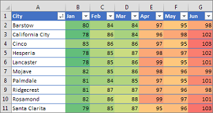
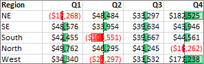
Color cells by value excel - Word и Excel - помощь в работе с программами

Conditional formatting can help make patterns and trends in your data more apparent. To use it, you create rules that determine the format of cells based on their values, such as the following monthly temperature data with cell colors tied to cell values.

You can apply conditional formatting to a range of cells (either a selection or a named range), an Excel table, and in Excel for Windows, even a PivotTable report.

Conditional formatting typically works the same way in a range of cells, an Excel table, or a PivotTable report. However, conditional formatting in a PivotTable report has some extra considerations:

There are some conditional formats that don’t work with fields in the Values area of a PivotTable report. For example, you can’t format such fields based on whether they contain unique or duplicate values. These restrictions are mentioned in the remaining sections of this article, where applicable.
If you change the layout of the PivotTable report by filtering, hiding levels, collapsing and expanding levels, or moving a field, the conditional format is maintained as long as the fields in the underlying data are not removed.
The scope of the conditional format for fields in the Values area can be based on the data hierarchy and is determined by all the visible children (the next lower level in a hierarchy) of a parent (the next higher level in a hierarchy) on rows for one or more columns, or columns for one or more rows.

Note: In the data hierarchy, children do not inherit conditional formatting from the parent, and the parent does not inherit conditional formatting from the children.
There are three methods for scoping the conditional format of fields in the Values area: by selection, by corresponding field, and by value field.

The default method of scoping fields in the Values area is by selection. You can change the scoping method to the corresponding field or value field by using the Apply formatting rule to option button, the New Formatting Rule dialog box, or the Edit Formatting Rule dialog box.

Method	Use this method if you want to select
Scoping by selection	A contiguous set of fields in the Values area, such as all of the product totals for one region. A non-contiguous set of fields in the Values area, such as product totals for different regions across levels in the data hierarchy.
Scoping by value field	Avoid making many non-contiguous selections. Conditionally format a set of fields in the Values area for all levels in the hierarchy of data. Include subtotals and grand totals.
Scoping by corresponding field	Avoid making many non-contiguous selections. Conditionally format a set of fields in the Values area for one level in the hierarchy of data. Exclude subtotals. When you conditionally format fields in the Values area for top, bottom, above average, or below average values, the rule is based on all visible values by default. However, when you scope by corresponding field, instead of using all visible values, you can apply the conditional format for each combination of: A column and its parent row field. A row and its parent column field.

Note: Quick Analysis is not available in Excel 2010 and previous versions.

Use the Quick Analysis button to apply selected conditional formatting to the selected data. The Quick Analysis button appears automatically when you select data.

Select the data that you want to conditionally format. The Quick Analysis button appears on the lower-right corner of the selection.
Click the Quick Analysis button , or press Ctrl+Q.
In the pop-up that appears, on the Formatting tab, move your mouse over the different options to see a Live Preview on your data, and then click on the formatting option you want.
Notes:
- The formatting options that appear in the Formatting tab depend on the data you have selected. If your selection contains only text, then the available options are Text, Duplicate, Unique, Equal To, and Clear. When the selection contains only numbers, or both text and numbers, then the options are Data Bars, Colors, Icon Sets, Greater, Top 10%, and Clear.
- Live preview will only render for those formatting options that can be used on your data. For example, if your selected cells don’t contain matching data and you select Duplicate, the live preview will not work.
If the Text that Contains dialog box appears, enter the formatting option you want to apply and click OK.

If you’d like to watch a video that shows how to use Quick Analysis to apply conditional formatting, see Video: Use conditional formatting.

You can download a sample workbook that contains different examples of applying conditional formatting, both with standard rules such as top and bottom, duplicates, Data Bars, Icon Sets and Color Scales, as well as manually creating rules of your own.

Download: Conditional formatting examples in Excel

Color scales are visual guides that help you understand data distribution and variation. A two-color scale helps you compare a range of cells by using a gradation of two colors. The shade of the color represents higher or lower values. For example, in a green and yellow color scale, as shown below, you can specify that higher value cells have a more green color and lower value cells have a more yellow color.

Tip: You can sort cells that have this format by their color — just use the context menu.

Tip: If any cells in the selection contain a formula that returns an error, the conditional formatting is not applied to those cells. To ensure that the conditional formatting is applied to those cells, use an IS or IFERROR function to return a value other than an error value.

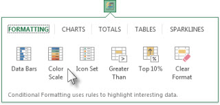
Quick formatting

Select one or more cells in a range, table, or PivotTable report.
On the Home tab, in the Styles group, click the arrow next to Conditional Formatting, and then click Color Scales.
Select a two-color scale.

Hover over the color scale icons to see which icon is a two-color scale. The top color represents higher values, and the bottom color represents lower values.

You can change the method of scoping for fields in the Values area of a PivotTable report by using the Formatting Options button that appears next to a PivotTable field that has conditional formatting applied.

Advanced formatting

Select one or more cells in a range, table, or PivotTable report.
On the Home tab, in the Styles group, click the arrow next to Conditional Formatting, and then click Manage Rules. The Conditional Formatting Rules Manager dialog box appears.
Do one of the following:
- To add a completely new conditional format, click New Rule. The New Formatting Rule dialog box appears.
- To add a new conditional format based on one that is already listed, select the rule, then click Duplicate Rule. The duplicate rule appears in the dialog box. Select the duplicate, then select Edit Rule. The Edit Formatting Rule dialog box appears.
- To change a conditional format, do the following:
  1. Make sure that the appropriate worksheet, table, or PivotTable report is selected in the Show formatting rules for list box.
  2. Optionally, change the range of cells by clicking Collapse Dialog in the Applies to box to temporarily hide the dialog box, by selecting the new range of cells on the worksheet, and then by selecting Expand Dialog.
  3. Select the rule, and then click Edit rule. The Edit Formatting Rule dialog box appears.
Under Apply Rule To, to optionally change the scope for fields in the Values area of a PivotTable report by:
- Selection: Click Selected cells.
- All cells for a Value label: Click All cells showing <Value label> values.
- All cells for a Value label, excluding subtotals and the grand total: Click All cells showing <Value label> values for <Row Label>.
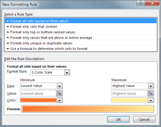
Under Select a Rule Type, click Format all cells based on their values (default).
Under Edit the Rule Description, in the Format Style list box, select 2-Color Scale.
To select a type in the Type box for Minimum and Maximum, do one of the following:
- Format lowest and highest values: Select Lowest Value and Highest Value.
  
  In this case, you do not enter a Minimum and MaximumValue.
- Format a number, date, or time value: Select Number and then enter a Minimum and MaximumValue.
- Format a percentage Percent: Enter a Minimum and MaximumValue.
  
  Valid values are from 0 (zero) to 100. Don’t enter a percent sign.
  
  Use a percentage when you want to visualize all values proportionally because the distribution of values is proportional.
- Format a percentile: Select Percentile and then enter a Minimum and MaximumValue. Valid percentiles are from 0 (zero) to 100.
  
  Use a percentile when you want to visualize a group of high values (such as the top 20thpercentile) in one color grade proportion and low values (such as the bottom 20th percentile) in another color grade proportion, because they represent extreme values that might skew the visualization of your data.
- Format a formula result: Select Formula and then enter values for Minimum and Maximum.
  - The formula must return a number, date, or time value.
  - Start the formula with an equal sign (=).
  - Invalid formulas result in no formatting being applied.
  - It’s a good idea to test the formula to make sure that it doesn’t return an error value.
    Notes:
    - Make sure that the Minimum value is less than the Maximum value.
    - You can choose a different type for the Minimum and Maximum. For example, you can choose a number for Minimum a percentage for Maximum.
To choose a Minimum and Maximum color scale, click Color for each, and then select a color.

If you want to choose additional colors or create a custom color, click More Colors. The color scale you select is shown in the Preview box.

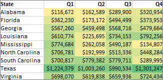
Color scales are visual guides that help you understand data distribution and variation. A three-color scale helps you compare a range of cells by using a gradation of three colors. The shade of the color represents higher, middle, or lower values. For example, in a green, yellow, and red color scale, you can specify that higher value cells have a green color, middle value cells have a yellow color, and lower value cells have a red color.

Tip: You can sort cells that have this format by their color — just use the context menu.

Quick formatting

Select one or more cells in a range, table, or PivotTable report.
On the Home tab, in the Styles group, click the arrow next to Conditional Formatting, and then click Color Scales.
Select a three-color scale. The top color represents higher values, the center color represents middle values, and the bottom color represents lower values.

Hover over the color scale icons to see which icon is a three-color scale.

Advanced formatting

Select one or more cells in a range, table, or PivotTable report.
On the Home tab, in the Styles group, click the arrow next to Conditional Formatting, and then click Manage Rules. The Conditional Formatting Rules Manager dialog box appears.
Do one of the following:
- To add a new conditional format, click New Rule. The New Formatting Rule dialog box appears.
- To add a new conditional format based on one that is already listed, select the rule, then click Duplicate Rule. The duplicate rule is copied and appears in the dialog box. Select the duplicate, then select Edit Rule. The Edit Formatting Rule dialog box appears.
- To change a conditional format, do the following:
  1. Make sure that the appropriate worksheet, table, or PivotTable report is selected in the Show formatting rules for list box.
  2. Optionally, change the range of cells by clicking Collapse Dialog in the Applies to box to temporarily hide the dialog box, by selecting the new range of cells on the worksheet, and then by selecting Expand Dialog.
  3. Select the rule, and then click Edit rule. The Edit Formatting Rule dialog box appears.
Under Apply Rule To, to optionally change the scope for fields in the Values area of a PivotTable report by:
- Selection: Click Just these cells.
- Corresponding field: Click All <value field> cells with the same fields.
- Value field: Click All <value field> cells.
Under Select a Rule Type, click Format all cells based on their values.
Under Edit the Rule Description, in the Format Style list box, select 3-Color Scale.
Select a type for Minimum, Midpoint, and Maximum. Do one of the following:
- Format lowest and highest values: Select a Midpoint.
  
  In this case, you do not enter a Lowest and HighestValue.
- Format a number, date, or time value: Select Number and then enter a value for Minimum, Midpoint, and Maximum.
- Format a percentage: Select Percent and then enter a value for Minimum, Midpoint, and Maximum. Valid values are from 0 (zero) to 100. Do not enter a percent (%) sign.
  
  Use a percentage when you want to visualize all values proportionally, because using a percentage ensures that the distribution of values is proportional.
- Format a percentile: Select Percentile and then enter a value for Minimum, Midpoint, and Maximum.
  
  Valid percentiles are from 0 (zero) to 100.
  
  Use a percentile when you want to visualize a group of high values (such as the top 20th percentile) in one color grade proportion and low values (such as the bottom 20th percentile) in another color grade proportion, because they represent extreme values that might skew the visualization of your data.
- Format a formula result: Select Formula and then enter a value for Minimum, Midpoint, and Maximum.
  
  The formula must return a number, date, or time value. Start the formula with an equal sign (=). Invalid formulas result in no formatting being applied. It’s a good idea to test the formula to make sure that it doesn’t return an error value.
  Notes:
  - You can set minimum, midpoint, and maximum values for the range of cells. Make sure that the value in Minimum is less than the value in Midpoint, which in turn is less than the value in Maximum.
  - You can choose a different type for Minimum, Midpoint, and Maximum. For example, you can choose a Minimum number, Midpoint percentile, and Maximum percent.
  - In many cases, the default Midpoint value of 50 percent works best, but you can adjust this to fit unique requirements.
To choose a Minimum, Midpoint, and Maximum color scale, click Color for each, and then select a color.
- To choose additional colors or create a custom color, click More Colors.
- The color scale you select is shown in the Preview box.

A data bar helps you see the value of a cell relative to other cells. The length of the data bar represents the value in the cell. A longer bar represents a higher value, and a shorter bar represents a lower value. Data bars are useful in spotting higher and lower numbers, especially with large amounts of data, such as top selling and bottom selling toys in a holiday sales report.

The example shown here uses data bars to highlight dramatic positive and negative values. You can format data bars so that the data bar starts in the middle of the cell, and stretches to the left for negative values.

Tip: If any cells in the range contain a formula that returns an error, the conditional formatting is not applied to those cells. To ensure that the conditional formatting is applied to those cells, use an IS or IFERROR function to return a value (such as 0 or «N/A») instead of an error value.

Quick formatting

Select one or more cells in a range, table, or PivotTable report.
On the Home tab, in the Style group, click the arrow next to Conditional Formatting, click Data Bars, and then select a data bar icon.

You can change the method of scoping for fields in the Values area of a PivotTable report by using the Apply formatting rule to option button.

Advanced formatting

Select one or more cells in a range, table, or PivotTable report.
On the Home tab, in the Styles group, click the arrow next to Conditional Formatting, and then click Manage Rules. The Conditional Formatting Rules Manager dialog box appears.
Do one of the following:
- To add a conditional format, click New Rule. The New Formatting Rule dialog box appears.
- To add a new conditional format based on one that is already listed, select the rule, then click Duplicate Rule. The duplicate rule is copied and appears in the dialog box. Select the duplicate, then select Edit Rule. The Edit Formatting Rule dialog box appears.
- To change a conditional format, do the following:
- 1. Make sure that the appropriate worksheet, table, or PivotTable report is selected in the Show formatting rules for list box.
  2. Optionally, change the range of cells by clicking Collapse Dialog in the Applies to box to temporarily hide the dialog box, by selecting the new range of cells on the worksheet, and then by selecting Expand Dialog.
  3. Select the rule, and then click Edit rule. The Edit Formatting Rule dialog box appears.
Under Apply Rule To, to optionally change the scope for fields in the Values area of a PivotTable report by:
- Selection: Click Just these cells.
- Corresponding field: Click All <value field> cells with the same fields.
- Value field: Click All <value field> cells.
Under Select a Rule Type, click Format all cells based on their values.
Under Edit the Rule Description, in the Format Style list box, select Data Bar.
Select a Minimum and MaximumType. Do one of the following:
- Format lowest and highest values: Select Lowest Value and Highest Value.
  
  In this case, you do not enter a value for Minimum and Maximum.
- Format a number, date, or time value: Select Number and then enter a Minimum and MaximumValue.
- Format a percentage: Select Percent and then enter a value for Minimum and Maximum.
  
  Valid values are from 0 (zero) to 100. Do not enter a percent (%) sign.
  
  Use a percentage when you want to visualize all values proportionally, because using a percentage ensures that the distribution of values is proportional.
- Format a percentile Select Percentile and then enter a value for Minimum and Maximum.
  
  Valid percentiles are from 0 (zero) to 100.
  
  Use a percentile when you want to visualize a group of high values (such as the top 20th percentile) in one data bar proportion and low values (such as the bottom 20th percentile) in another data bar proportion, because they represent extreme values that might skew the visualization of your data.
- Format a formula result Select Formula, and then enter a value for Minimum and Maximum.
  - The formula has to return a number, date, or time value.
  - Start the formula with an equal sign (=).
  - Invalid formulas result in no formatting being applied.
  - It’s a good idea to test the formula to make sure that it doesn’t return an error value.
Notes:
- Make sure that the Minimum value is less than the Maximum value.
- You can choose a different type for Minimum and Maximum. For example, you can choose a Minimum number and a Maximum percent.
To choose a Minimum and Maximum color scale, click Bar Color.

If you want to choose additional colors or create a custom color, click More Colors. The bar color you select is shown in the Preview box.
To show only the data bar and not the value in the cell, select Show Bar Only.
To apply a solid border to data bars, select Solid Border in the Border list box and choose a color for the border.
To choose between a solid bar and a gradiated bar, choose Solid Fill or Gradient Fill in the Fill list box.
To format negative bars, click Negative Value and Axis and then, in the Negative Value and Axis Settings dialog box, choose options for the negative bar fill and border colors. You can choose position settings and a color for the axis. When you are finished selecting options, click OK.
You can change the direction of bars by choosing a setting in the Bar Direction list box. This is set to Context by default, but you can choose between a left-to-right and a right-to-left direction, depending on how you want to present your data.

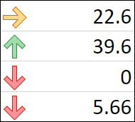
Use an icon set to annotate and classify data into three to five categories separated by a threshold value. Each icon represents a range of values. For example, in the 3 Arrows icon set, the green up arrow represents higher values, the yellow sideways arrow represents middle values, and the red down arrow represents lower values.

Tip: You can sort cells that have this format by their icon — just use the context menu.

The example shown here works with several examples of conditional formatting icon sets.

You can choose to show icons only for cells that meet a condition; for example, displaying a warning icon for those cells that fall below a critical value and no icons for those that exceed it. To do this, you hide icons by selecting No Cell Icon from the icon drop-down list next to the icon when you are setting conditions. You can also create your own combination of icon sets; for example, a green «symbol» check mark, a yellow «traffic light», and a red «flag.»

Quick formatting

Select the cells that you want to conditionally format.
On the Home tab, in the Style group, click the arrow next to Conditional Formatting, click Icon Set, and then select an icon set.

You can change the method of scoping for fields in the Values area of a PivotTable report by using the Apply formatting rule to option button.

Advanced formatting

Select the cells that you want to conditionally format.
On the Home tab, in the Styles group, click the arrow next to Conditional Formatting, and then click Manage Rules. The Conditional Formatting Rules Manager dialog box appears.
Do one of the following:
- To add a conditional format, click New Rule. The New Formatting Rule dialog box appears.
- To add a new conditional format based on one that is already listed, select the rule, then click Duplicate Rule. The duplicate rule is copied and appears in the dialog box. Select the duplicate, then select Edit Rule. The Edit Formatting Rule dialog box appears.
- To change a conditional format, do the following:
  1. Make sure that the appropriate worksheet, table, or PivotTable report is selected in the Show formatting rules for list box.
  2. Optionally, change the range of cells by clicking Collapse Dialog in the Applies to box to temporarily hide the dialog box, by selecting the new range of cells on the worksheet, and then by selecting Expand Dialog.
  3. Select the rule, and then click Edit rule. The Edit Formatting Rule dialog box appears.
Under Apply Rule To, to optionally change the scope for fields in the Values area of a PivotTable report by:
- Selection: Click Just these cells.
- Corresponding field: Click All <value field> cells with the same fields.
- Value field: Click All <value field> cells.
Under Select a Rule Type, click Format all cells based on their values.
Under Edit the Rule Description, in the Format Style list box, select Icon Set.
1. Select an icon set. The default is 3 Traffic Lights (Unrimmed). The number of icons and the default comparison operators and threshold values for each icon can vary for each icon set.
2. You can adjust the comparison operators and threshold values. The default range of values for each icon are equal in size, but you can adjust these to fit your unique requirements. Make sure that the thresholds are in a logical sequence of highest to lowest from top to bottom.
3. Do one of the following:
  - Format a number, date, or time value: Select Number.
  - Format a percentage: Select Percent.
    
    Valid values are from 0 (zero) to 100. Do not enter a percent (%) sign.
    
    Use a percentage when you want to visualize all values proportionally, because using a percentage ensures that the distribution of values is proportional.
  - Format a percentile: Select Percentile. Valid percentiles are from 0 (zero) to 100.
    
    Use a percentile when you want to visualize a group of high values (such as the top 20th percentile) using a particular icon and low values (such as the bottom 20th percentile) using another icon, because they represent extreme values that might skew the visualization of your data.
  - Format a formula result: Select Formula, and then enter a formula in each Value box.
    - The formula must return a number, date, or time value.
    - Start the formula with an equal sign (=).
    - Invalid formulas result in no formatting being applied.
    - It’s a good idea to test the formula to make sure that it doesn’t return an error value.
4. To make the first icon represent lower values and the last icon represent higher values, select Reverse Icon Order.
5. To show only the icon and not the value in the cell, select Show Icon Only.
  Notes:
  - You may need to adjust the column width to accommodate the icon.
  - The size of the icon shown depends on the font size that is used in that cell. As the size of the font is increased, the size of the icon increases proportionally.

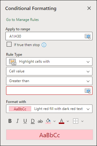
To more easily find specific cells, you can format them by using a comparison operator. For example, in an inventory worksheet sorted by categories, you could highlight products with fewer than 10 items on hand in yellow. Or, in a retail store summary worksheet, you might identify all stores with profits greater than 10%, sales volumes less than $100,000, and region equal to «SouthEast.»

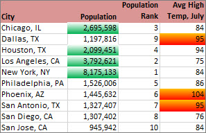
The examples shown here work with examples of built-in conditional formatting criteria, such as Greater Than, and Top %. This formats cities with a population greater than 2,000,000 with a green background and average high temperatures in the top 30% with orange.

Note: You cannot conditionally format fields in the Values area of a PivotTable report by text or by date, only by number.

Quick formatting

Select one or more cells in a range, table, or PivotTable report.
On the Home tab, in the Style group, click the arrow next to Conditional Formatting, and then click Highlight Cells Rules.
Select the command you want, such as Between, Equal To Text that Contains, or A Date Occurring.
Enter the values you want to use, and then select a format.

You can change the method of scoping for fields in the Values area of a PivotTable report by using the Apply formatting rule to option button.

If you’d like to watch videos of these techniques, see Video: Conditionally format text and Video: Conditionally format dates.

Advanced formatting

Select one or more cells in a range, table, or PivotTable report.
On the Home tab, in the Styles group, click the arrow next to Conditional Formatting, and then click Manage Rules. The Conditional Formatting Rules Manager dialog box appears.
Do one of the following:
- To add a conditional format, click New Rule. The New Formatting Rule dialog box appears.
- To add a new conditional format based on one that is already listed, select the rule, then click Duplicate Rule. The duplicate rule is copied and appears in the dialog box. Select the duplicate, then select Edit Rule. The Edit Formatting Rule dialog box appears.
- To change a conditional format, do the following:
- 1. Make sure that the appropriate worksheet, table, or PivotTable report is selected in the Show formatting rules for list box.
  2. Optionally, change the range of cells by clicking Collapse Dialog in the Applies to box to temporarily hide the dialog box, by selecting the new range of cells on the worksheet or on other worksheets, and then by selecting Expand Dialog.
  3. Select the rule, and then click Edit rule. The Edit Formatting Rule dialog box appears.
Under Apply Rule To, to optionally change the scope for fields in the Values area of a PivotTable report by:
- Selection: Click Just these cells.
- Corresponding field: Click All <value field> cells with the same fields.
- Value field: Click All <value field> cells.
Under Select a Rule Type, click Format only cells that contain.
Under Edit the Rule Description, in the Format only cells with list box, do one of the following:
- Format by number, date, or time: Select Cell Value, select a comparison operator, and then enter a number, date, or time.
  
  For example, select Between and then enter 100 and 200, or select Equal to and then enter 1/1/2009.
  
  You can also enter a formula that returns a number, date, or time value.
  - If you enter a formula, start it with an equal sign (=).
  - Invalid formulas result in no formatting being applied.
  - It’s a good idea to test the formula to make sure that it doesn’t return an error value.
- Format by text: Select Specific Text, choosing a comparison operator, and then enter text.
  
  For example, select Contains and then enter Silver, or select Starting with and then enter Tri.
  
  Quotes are included in the search string, and you may use wildcard characters. The maximum length of a string is 255 characters.
  
  You can also enter a formula that returns text.
  - If you enter a formula, start it with an equal sign (=).
  - Invalid formulas result in no formatting being applied.
  - It’s a good idea to test the formula to make sure that it doesn’t return an error value.
  To see a video of this technique, see Video: Conditionally format text.
- Format by date: Select Dates Occurring and then select a date comparison.
  
  For example, select Yesterday or Next week.
  
  To see a video of this technique, see Video: Conditionally format dates.
- Format cells with blanks or no blanks: Select Blanks or No Blanks.
  
  A blank value is a cell that contains no data and is different from a cell that contains one or more spaces (spaces are considered as text).
- Format cells with error or no error values: Select Errors or No Errors.
  
  Error values include: #####, #VALUE!, #DIV/0!, #NAME?, #N/A, #REF!, #NUM!, and #NULL!.
To specify a format, click Format. The Format Cells dialog box appears.
Select the number, font, border, or fill format you want to apply when the cell value meets the condition, and then click OK.

You can choose more than one format. The formats you select are shown in the Preview box.

You can find the highest and lowest values in a range of cells that are based on a cutoff value you specify. For example, you can find the top 5 selling products in a regional report, the bottom 15% products in a customer survey, or the top 25 salaries in a department .

Quick formatting

Select one or more cells in a range, table, or PivotTable report.
On the Home tab, in the Style group, click the arrow next to Conditional Formatting, and then click Top/Bottom Rules.
Select the command you want, such as Top 10 items or Bottom 10 %.
Enter the values you want to use, and then select a format.

You can change the method of scoping for fields in the Values area of a PivotTable report by using the Apply formatting rule to option button.

Advanced formatting

Select one or more cells in a range, table, or PivotTable report.
On the Home tab, in the Styles group, click the arrow next to Conditional Formatting, and then click Manage Rules. The Conditional Formatting Rules Manager dialog box appears.
Do one of the following:
- To add a conditional format, click New Rule. The New Formatting Rule dialog box appears.
- To add a new conditional format based on one that is already listed, select the rule, then click Duplicate Rule. The duplicate rule is copied and appears in the dialog box. Select the duplicate, then select Edit Rule. The Edit Formatting Rule dialog box appears.
- To change a conditional format, do the following:
- 1. Make sure that the appropriate worksheet, table, or PivotTable report is selected in the Show formatting rules for list box.
  2. Optionally, change the range of cells by clicking Collapse Dialog in the Applies to box to temporarily hide the dialog box, by selecting the new range of cells on the worksheet, and then by selecting Expand Dialog.
  3. Select the rule, and then click Edit rule. The Edit Formatting Rule dialog box appears.
Under Apply Rule To, to optionally change the scope fields in the Values area of a PivotTable report by:
- Selection: Click Just these cells.
- Corresponding field: Click All <value field> cells with the same fields.
- Value field: Click All <value field> cells.
Under Select a Rule Type, click Format only top or bottom ranked values.
Under Edit the Rule Description, in the Format values that rank in the list box, select Top or Bottom.
Do one of the following:
- To specify a top or bottom number, enter a number and then clear the % of the selected range box. Valid values are 1 to 1000.
- To specify a top or bottom percentage, enter a number and then select the % of the selected range box. Valid values are 1 to 100.
Optionally, change how the format is applied for fields in the Values area of a PivotTable report that are scoped by corresponding field.

By default, the conditional format is based on all visible values. However when you scope by corresponding field, instead of using all visible values, you can apply the conditional format for each combination of:
- A column and its parent row field, by selecting each Column group.
- A row and its parent column field, by selecting each Row group.
To specify a format, click Format. The Format Cells dialog box appears.
Select the number, font, border, or fill format you want to apply when the cell value meets the condition, and then click OK.

You can choose more than one format. The formats you select are shown in the Preview box.

You can find values above or below an average or standard deviation in a range of cells. For example, you can find the above average performers in an annual performance review or you can locate manufactured materials that fall below two standard deviations in a quality rating.

Quick formatting

Select one or more cells in a range, table, or PivotTable report.
On the Home tab, in the Style group, click the arrow next to Conditional Formatting, and then click Top/Bottom Rules.
Select the command you want, such as Above Average or Below Average.
Enter the values you want to use, and then select a format.

You can change the method of scoping for fields in the Values area of a PivotTable report by using the Apply formatting rule to option button.

Advanced formatting

Select one or more cells in a range, table, or PivotTable report.
On the Home tab, in the Styles group, click the arrow next to Conditional Formatting, and then click Manage Rules. The Conditional Formatting Rules Manager dialog box appears.
Do one of the following:
- To add a conditional format, click New Rule. The New Formatting Rule dialog box appears.
- To add a new conditional format based on one that is already listed, select the rule, then click Duplicate Rule. The duplicate rule is copied and appears in the dialog box. Select the duplicate, then select Edit Rule. The Edit Formatting Rule dialog box appears.
- To change a conditional format, do the following:
- 1. Make sure that the appropriate worksheet, table, or PivotTable report is selected in the Show formatting rules for list box.
  2. Optionally, change the range of cells by clicking Collapse Dialog in the Applies to box to temporarily hide the dialog box, by selecting the new range of cells on the worksheet, and then by selecting Expand Dialog.
  3. Select the rule, and then click Edit rule. The Edit Formatting Rule dialog box appears.
Under Apply Rule To, to optionally change the scope for fields in the Values area of a PivotTable report by:
- Selection: Click Just these cells.
- Corresponding field: Click All <value field> cells with the same fields.
- Value field: Click All <value field> cells.
Under Select a Rule Type, click Format only values that are above or below average.
Under Edit the Rule Description, in the Format values that are list box, do one of the following:
- To format cells that are above or below the average for all of the cells in the range, select Above or Below.
- To format cells that are above or below one, two, or three standard deviations for all of the cells in the range, select a standard deviation.
Optionally, change how the format is applied for fields in the Values area of a PivotTable report that are scoped by corresponding field.

By default, the conditionally format is based on all visible values. However when you scope by corresponding field, instead of using all visible values, you can apply the conditional format for each combination of:
- A column and its parent row field, by selecting each Column group.
- A row and its parent column field, by selecting each Row group.
Click Format to display the Format Cells dialog box.
Select the number, font, border, or fill format you want to apply when the cell value meets the condition, and then click OK.

You can choose more than one format. The formats you select are displayed in the Preview box.

Note: You can’t conditionally format fields in the Values area of a PivotTable report by unique or duplicate values.

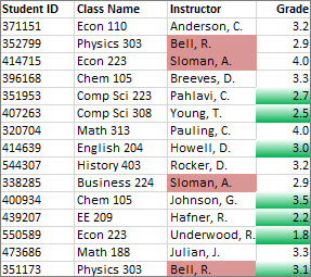
In the example shown here, conditional formatting is used on the Instructor column to find instructors that are teaching more than one class (duplicate instructor names are highlighted in a pale red color). Grade values that are found just once in the Grade column (unique values) are highlighted in a green color.

Quick formatting

Select the cells that you want to conditionally format.
On the Home tab, in the Style group, click the arrow next to Conditional Formatting, and then click Highlight Cells Rules.
Select Duplicate Values.
Enter the values you want to use, and then select a format.

Advanced formatting

Select the cells that you want to conditionally format.
On the Home tab, in the Styles group, click the arrow next to Conditional Formatting, and then click Manage Rules. The Conditional Formatting Rules Manager dialog box appears.
Do one of the following:
- To add a conditional format, click New Rule. The New Formatting Rule dialog box appears.
- To add a new conditional format based on one that is already listed, select the rule, then click Duplicate Rule. The duplicate rule is copied and appears in the dialog box. Select the duplicate, then select Edit Rule. The Edit Formatting Rule dialog box appears.
- To change a conditional format, do the following:
- 1. Make sure that the appropriate worksheet or table is selected in the Show formatting rules for list box.
  2. Optionally, change the range of cells by clicking Collapse Dialog in the Applies to box to temporarily hide the dialog box, by selecting the new range of cells on the worksheet, and then by selecting Expand Dialog.
  3. Select the rule, and then click Edit rule. The Edit Formatting Rule dialog box appears.
Under Select a Rule Type, click Format only unique or duplicate values.
Under Edit the Rule Description, in the Format all list box, select unique or duplicate.
Click Format to display the Format Cells dialog box.
Select the number, font, border, or fill format you want to apply when the cell value meets the condition, and then click OK.

You can choose more than one format. The formats you select are shown in the Preview box.

If none of the above options is what you’re looking for, you can create your own conditional formatting rule in a few simple steps.

Notes: If there’s already a rule defined that you just want to work a bit differently, duplicate the rule and edit it.

Select Home > Conditional Formatting > Manage Rules, then in the Conditional Formatting Rule Manager dialog, select a listed rule and then select Duplicate Rule. The duplicate rule then appears in the list.
Select the duplicate rule, then select Edit Rule.

Select the cells that you want to format.
On the Home tab, click Conditional Formatting > New Rule.
Create your rule and specify its format options, then click OK.

If you don’t see the options that you want, you can use a formula to determine which cells to format — see the next section for steps).

If you don’t see the exact options you need when you create your own conditional formatting rule, you can use a logical formula to specify the formatting criteria. For example, you may want to compare values in a selection to a result returned by a function or evaluate data in cells outside the selected range, which can be in another worksheet in the same workbook. Your formula must return True or False (1 or 0), but you can use conditional logic to string together a set of corresponding conditional formats, such as different colors for each of a small set of text values (for example, product category names).

Note: You can enter cell references in a formula by selecting cells directly on a worksheet or other worksheets. Selecting cells on the worksheet inserts absolute cell references. If you want Excel to adjust the references for each cell in the selected range, use relative cell references. For more information, see Create or change a cell reference and Switch between relative, absolute, and mixed references.

Tip: If any cells contain a formula that returns an error, conditional formatting is not applied to those cells. To address this, use IS functions or an IFERROR function in your formula to return a value that you specify (such as 0, or «N/A») instead of an error value.

On the Home tab, in the Styles group, click the arrow next to Conditional Formatting, and then click Manage Rules.

The Conditional Formatting Rules Manager dialog box appears.
Do one of the following:
- To add a conditional format, click New Rule. The New Formatting Rule dialog box appears.
- To add a new conditional format based on one that is already listed, select the rule, then click Duplicate Rule. The duplicate rule is copied and appears in the dialog box. Select the duplicate, then select Edit Rule. The Edit Formatting Rule dialog box appears.
- To change a conditional format, do the following:
- 1. Make sure that the appropriate worksheet, table, or PivotTable report is selected in the Show formatting rules for list box.
  2. Optionally, change the range of cells by clicking Collapse Dialog in the Applies to box to temporarily hide the dialog box, by selecting the new range of cells on the worksheet or other worksheets, and then by clicking Expand Dialog.
  3. Select the rule, and then click Edit rule. The Edit Formatting Rule dialog box appears.
Under Apply Rule To, to optionally change the scope for fields in the Values area of a PivotTable report, do the following:
- To scope by selection: Click Selected cells.
- To scope by corresponding field: Click All cells showing <Values field> values.
- To scope by Value field: Click All cells showing <Values field> for <Row>.

Under Select a Rule Type, click Use a formula to determine which cells to format.

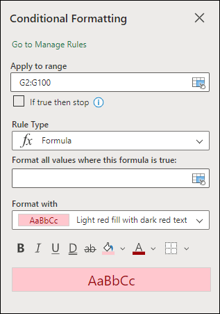
Under Edit the Rule Description, in the Format values where this formula is true list box, enter a formula.

You have to start the formula with an equal sign (=), and the formula must return a logical value of TRUE (1) or FALSE (0).
Click Format to display the Format Cells dialog box.

Select the number, font, border, or fill format you want to apply when the cell value meets the condition, and then click OK.

You can choose more than one format. The formats you select are shown in the Preview box.

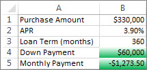
Example 1: Use two conditional formats with criteria that uses AND and OR tests

The following example shows the use of two conditional formatting rules. If the first rule doesn’t apply, the second rule applies.

First rule: a home buyer has budgeted up to $75,000 as a down payment and $1,500 per month as a mortgage payment. If both the down payment and the monthly payments fit these requirements, cells B4 and B5 are formatted green.

Second rule: if either the down payment or the monthly payment doesn’t meet the buyer’s budget, B4 and B5 are formatted red. Change some values, such as the APR, the loan term, the down payment, and the purchase amount to see what happens with the conditionally formatted cells.

Formula for first rule (applies green color)	=AND(IF($B$4<=75000,1),IF(ABS($B$5)<=1500,1))
Formula for second rule (applies red color)	=OR(IF($B$4>=75000,1),IF(ABS($B$5)>=1500,1))

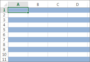
Example 2: Shade every other row by using the MOD and ROW functions

A conditional format applied to every cell in this worksheet shades every other row in the range of cells with a blue cell color. You can select all cells in a worksheet by clicking the square above row 1 and to the left of column A. The MOD function returns a remainder after a number (the first argument) is divided by divisor (the second argument). The ROW function returns the current row number. When you divide the current row number by 2, you always get either a 0 remainder for an even number or a 1 remainder for an odd number. Because 0 is FALSE and 1 is TRUE, every odd numbered row is formatted. The rule uses this formula: =MOD(ROW(),2)=1.

The following video shows you the basics of using formulas with conditional formatting.

If you want to apply an existing formatting style to new or other data on your worksheet, you can use Format Painter to copy the conditional formatting to that data.

Click the cell that has the conditional formatting that you want to copy.
Click Home > Format Painter.

The pointer changes to a paintbrush.

Tip: You can double-click Format Painter if you want to keep using the paintbrush to paste the conditional formatting in other cells.
To paste the conditional formatting, drag the paintbrush across the cells or ranges of cells you want to format.
To stop using the paintbrush, press Esc.

Note: If you’ve used a formula in the rule that applies the conditional formatting, you might have to adjust any cell references in the formula after pasting the conditional format. For more information, see Switch between relative, absolute, and mixed references.

If your worksheet contains conditional formatting, you can quickly locate the cells so that you can copy, change, or delete the conditional formats. Use the Go To Special command to find only cells with a specific conditional format, or to find all cells that have conditional formats.

Find all cells that have a conditional format

Click any cell that does not have a conditional format.
On the Home tab, in the Editing group, click the arrow next to Find & Select, and then click Conditional Formatting.

Find only cells that have the same conditional format

Click any cell that has the conditional format that you want to find.
On the Home tab, in the Editing group, click the arrow next to Find & Select, and then click Go To Special.
Click Conditional formats.
Click Same under Data validation.

When you use conditional formatting, you set up rules that Excel uses to determine when to apply the conditional formatting. To manage these rules, you should understand the order in which these rules are evaluated, what happens when two or more rules conflict, how copying and pasting can affect rule evaluation, how to change the order in which rules are evaluated, and when to stop rule evaluation.

Learn about conditional formatting rule precedence

You create, edit, delete, and view all conditional formatting rules in the workbook by using the Conditional Formatting Rules Manager dialog box. (On the Home tab, click Conditional Formatting, and then click Manage Rules.)

The Conditional Formatting Rules Manager dialog box appears.

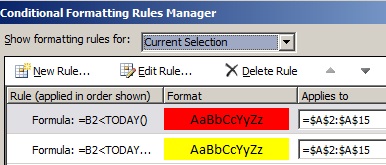
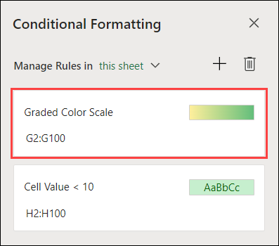
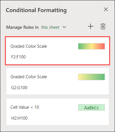
When two or more conditional formatting rules apply, these rules are evaluated in order of precedence (top to bottom) by how they are listed in this dialog box.

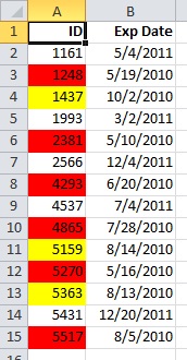
Here’s an example that has expiration dates for ID badges. We want to mark badges that expire within 60 days but are not yet expired with a yellow background color, and expired badges with a red background color.

In this example, cells with employee ID numbers who have certification dates due to expire within 60 days are formatted in yellow, and ID numbers of employees with an expired certification are formatted in red. The rules are shown in the following image.

The first rule (which, if True, sets cell background color to red) tests a date value in column B against the current date (obtained by using the TODAY function in a formula). Assign the formula to the first data value in column B, which is B2. The formula for this rule is =B2<TODAY(). This formula tests the cells in column B (cells B2:B15). If the formula for any cell in column B evaluates to True, its corresponding cell in column A (for example, A5 corresponds to B5, A11 corresponds to B11), is then formatted with a red background color. After all the cells specified under Applies to are evaluated with this first rule, the second rule is tested. This formula checks if values in the B column are less than 60 days from the current date (for example, suppose today’s date is 8/11/2010). The cell in B4, 10/4/2010, is less than 60 days from today, so it evaluates as True, and is formatted with a yellow background color. The formula for this rule is =B2<TODAY()+60. Any cell that was first formatted red by the highest rule in the list is left alone.

A rule higher in the list has greater precedence than a rule lower in the list. By default, new rules are always added to the top of the list and therefore have a higher precedence, so you’ll want to keep an eye on their order. You can change the order of precedence by using the Move Up and Move Down arrows in the dialog box.
What happens when more than one conditional formatting rule evaluates to True

Sometimes you have more than one conditional formatting rule that evaluates to True. Here’s how rules are applied, first when rules don’t conflict, and then when they do conflict:

When rules don’t conflict For example, if one rule formats a cell with a bold font and another rule formats the same cell with a red color, the cell is formatted with both a bold font and a red color. Because there is no conflict between the two formats, both rules are applied.

When rules conflict For example, one rule sets a cell font color to red and another rule sets a cell font color to green. Because the two rules are in conflict, only one can apply. The rule that is applied is the one that is higher in precedence (higher in the list in the dialog box).
How pasting, filling, and the Format Painter affect conditional formatting rules

While editing your worksheet, you may copy and paste cell values that have conditional formats, fill a range of cells with conditional formats, or use the Format Painter. These operations can affect conditional formatting rule precedence in the following way: a new conditional formatting rule based on the source cells is created for the destination cells.

If you copy and paste cell values that have conditional formats to a worksheet opened in another instance of Excel (another Excel.exe process running at the same time on the computer), no conditional formatting rule is created in the other instance and the format is not copied to that instance.
What happens when a conditional format and a manual format conflict

If a conditional formatting rule evaluates as True, it takes precedence over any existing manual format for the same selection. This means that if they conflict, the conditional formatting applies and the manual format does not. If you delete the conditional formatting rule, the manual formatting for the range of cells remains.

Manual formatting is not listed in the Conditional Formatting Rules Manager dialog box nor is it used to determine precedence.

Controlling when rule evaluation stops by using the Stop If True check box

For backwards compatibility with versions of Excel earlier than Excel 2007, you can select the Stop If True check box in the Manage Rules dialog box to simulate how conditional formatting might appear in those earlier versions of Excel that do not support more than three conditional formatting rules or multiple rules applied to the same range.

For example, if you have more than three conditional formatting rules for a range of cells, and are working with a version of Excel earlier than Excel 2007, that version of Excel:

Evaluates only the first three rules.
Applies the first rule in precedence that is True.
Ignores rules lower in precedence if they are True.

The following table summarizes each possible condition for the first three rules:

If rule	Is	And if rule	Is	And if rule	Is	Then
One	True	Two	True or False	Three	True or False	Rule one is applied and rules two and three are ignored.
One	False	Two	True	Three	True or False	Rule two is applied and rule three is ignored.
One	False	Two	False	Three	True	Rule three is applied.
One	False	Two	False	Three	False	No rules are applied.

You can select or clear the Stop If True check box to change the default behavior:

To evaluate only the first rule, select the Stop If True check box for the first rule.
To evaluate only the first and second rules, select the Stop If True check box for the second rule.

You can’t select or clear the Stop If True check box if the rule formats by using a data bar, color scale, or icon set.

If you’d like to watch a video showing how to manage conditional formatting rules, see Video: Manage conditional formatting.

The order in which conditional formatting rules are evaluated — their precedence — also reflects their relative importance: the higher a rule is on the list of conditional formatting rules, the more important it is. This means that in cases where two conditional formatting rules conflict with each other, the rule that is higher on the list is applied and the rule that is lower on the list is not applied.

On the Home tab, in the Styles group, click the arrow next to Conditional Formatting, and then click Manage Rules.

The Conditional Formatting Rules Manager dialog box appears.

The conditional formatting rules for the current selection are displayed, including the rule type, the format, the range of cells the rule applies to, and the Stop If True setting.

If you don’t see the rule that you want, in the Show formatting rules for list box, make sure that the right range of cells, worksheet, table, or PivotTable report is selected.
Select a rule. Only one rule can be selected at a time.
To move the selected rule up in precedence, click Move Up. To move the selected rule down in precedence, click Move Down.
Optionally, to stop rule evaluation at a specific rule, select the Stop If True check box.

Clear conditional formatting on a worksheet

On the Home tab, click Conditional Formatting > Clear Rules > Clear Rules from Entire Sheet.

Follow these steps if you have conditional formatting in a worksheet, and you need to remove it.

For an entire
worksheet

On the Home tab, click Conditional Formatting > Clear Rules > Clear Rules from Entire Sheet.

In a range of cells

Select the cells that contain the conditional formatting.
Click the Quick Analysis Lens button that appears to the bottom right of the selected data.
Notes:
Quick Analysis Lens will not be visible if:
- All of the cells in the selected range are empty, or
- There is an entry only in the upper-left cell of the selected range, with all of the other cells in the range being empty.
Click Clear Format.

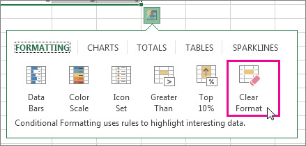
Find and remove the same conditional formats throughout a worksheet

Click on a cell that has the conditional format that you want to remove throughout the worksheet.
On the Home tab, click the arrow next to Find & Select, and then click Go To Special.
Click Conditional formats.
Click Same under Data validation. to select all of the cells that contain the same conditional formatting rules.
On the Home tab, click Conditional Formatting > Clear Rules > Clear Rules from Selected Cells.

Tip: The following sections use examples so you can follow along in Excel for the web. To start, download the Conditional Formatting Examples workbook and save it to OneDrive. Then, open OneDrive in a web browser and select the downloaded file.

Select the cells you want to format, then select Home > Styles > Conditional Formatting > New Rule. You can also open the Conditional Formatting pane and create a new rule without first selecting a range of cells.
Verify or adjust the cells in Apply to range.
Choose a Rule Type and adjust the options to meet your needs.
When finished, select Done and the rule will be applied to your range.

Select a cell which has a conditional format you want to change. Or you can select Home > Styles > Conditional Formatting > Manage Rules to open the Conditional Formatting task pane and select an existing rule.
The Conditional Formatting task pane displays any rules which apply to specific cells or ranges of cells.
Hover over the rule and select Edit by clicking the pencil icon. This opens the task pane for rule editing.
Modify the rule settings and click Done to apply the changes.

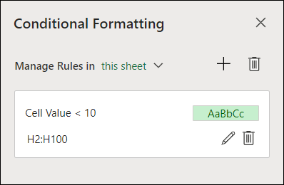
The Conditional Formatting task pane provides everything you need for creating, editing, and deleting rules. Use Manage Rules to open the task pane and work with all the Conditional Formatting rules in a selection or a sheet.

In an open workbook, select Home > Styles > Conditional Formatting > Manage Rules.
The Conditional Formatting task pane opens and displays the rules, scoped to your current selection.

From here, you can:

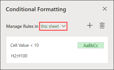
Choose a different scope on the Manage Rules in menu — for example, choosing this sheet tells Excel to look for all rules on the current sheet.
Add a rule by selecting New Rule (the plus sign).
Delete all rules in scope by selecting Delete All Rules (the garbage can).

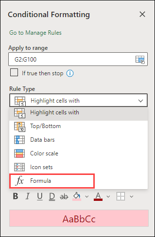
You can use a formula to determine how Excel evaluates and formats a cell. Open the Conditional Formatting pane and select an existing rule or create a new rule.

In the Rule Type dropdown, select Formula.

Enter the formula in the box. You can use any formula that returns a logical value of TRUE (1) or FALSE (0), but you can use AND and OR to combine a set of logical checks.

For example, =AND(B3=»Grain»,D3<500) is true for a cell in row 3 if both B3=»Grain» and D3<500 are true.

You can clear conditional formatting in selected cells or the entire worksheet.

To clear conditional formatting in selected cells, select the cells in the worksheet. Then Select Home > Styles > Conditional Formatting > Clear Rules > Clear Rules from Selected Cells.
To clear conditional formatting in the entire worksheet, select Home > Styles > Conditional Formatting > Clear Rules > Clear Rules from Entire Sheet.
To delete conditional formatting rules, select Home > Styles > Conditional Formatting >Manage Rules and use the delete (garbage can) on a specific rule or the Delete all rules button.

Color scales are visual guides which help you understand data distribution and variation. Excel offers both two-color scales and three-color scales.

A two-color scale helps you compare a range of cells by using a gradation of two colors. The shade of the color represents higher or lower values. For example, in a green and yellow color scale, you can specify that higher value cells be more green and lower value cells have a more yellow.

A three-color scale helps you compare a range of cells by using a gradation of three colors. The shade of the color represents higher, middle, or lower values. For example, in a green, yellow, and red color scale, you can specify that higher value cells have a green color, middle value cells have a yellow color, and lower value cells have a red color.

Tip: You can sort cells that have one of these formats by their color — just use the context menu.

Select the cells that you want to conditionally format using color scales.
Click Home > Styles > Conditional Formatting > Color Scales and select a color scale.

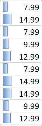
A data bar helps you see the value of a cell relative to other cells. The length of the data bar represents the value in the cell. A longer bar represents a higher value, and a shorter bar represents a lower value. Data bars are useful in spotting higher and lower numbers, especially with large amounts of data, such as top selling and bottom selling toys in a holiday sales report.

Select the cells that you want to conditionally format.
Select Home > Styles > Conditional Formatting > Data Bars and select a style.

Use an icon set to annotate and classify data into three to five categories separated by a threshold value. Each icon represents a range of values. For example, in the 3 Arrows icon set, the green up arrow represents higher values, the yellow sideways arrow represents middle values, and the red down arrow represents lower values.

Select the cells that you want to conditionally format.
Select Home > Styles > Conditional Formatting > Icon Sets and choose an icon set.

This option lets you highlight specific cell values within a range of cells based on their specific contents. This can be especially useful when working with data sorted using a different range.

For example, in an inventory worksheet sorted by categories, you could highlight the names of products where you have fewer than 10 items in stock so it’s easy to see which products need restocking without resorting the data.

Select the cells that you want to conditionally format.
Select Home > Styles > Conditional Formatting > Highlight Cell Rules.
Select the comparison, such as Between, Equal To, Text That Contains, or A Date Occurring.

You can highlight the highest and lowest values in a range of cells which are based on a specified cutoff value.

Some examples of this would include highlighting the top five selling products in a regional report, the bottom 15% products in a customer survey, or the top 25 salaries in a department.

Select the cells that you want to conditionally format.
Select Home > Styles > Conditional Formatting > Top/Bottom Rules.
Select the command you want, such as Top 10 items or Bottom 10 %.
Enter the values you want to use, and select a format (fill, text, or border color).

You can highlight values above or below an average or standard deviation in a range of cells.

For example, you can find the above-average performers in an annual performance review, or locate manufactured materials that fall below two standard deviations in a quality rating.

Select the cells that you want to conditionally format.
Select Home> Styles > Conditional Formatting > Top/Bottom Rules.
Select the option you want, such as Above Average or Below Average.
Enter the values you want to use, and select a format (fill, text, or border color).

Select the cells that you want to conditionally format.
Select Home > Styles > Conditional Formatting > Highlight Cell Rules > Duplicate Values.
Enter the values you want to use, and select a format (fill, text, or border color).

If you want to apply an existing formatting style to other cells on your worksheet, use Format Painter to copy the conditional formatting to that data.

Click the cell that has the conditional formatting you want to copy.
Click Home > Format Painter.

The pointer will change to a paintbrush.

Tip: You can double-click Format Painter if you want to keep using the paintbrush to paste the conditional formatting in other cells.
Drag the paintbrush across the cells or range of cells you want formatted.
To stop using the paintbrush, press Esc.

Note: If you’ve used a formula in the rule that applies the conditional formatting, you might have to adjust relative and absolute references in the formula after pasting the conditional format. For more information, see Switch between relative, absolute, and mixed references.

Note: You can’t use conditional formatting on external references to another workbook.

Need more help?

You can always ask an expert in the Excel Tech Community or get support in the Answers community.

Процедура изменения цвета ячеек в зависимости от содержимого

Конечно, всегда приятно иметь хорошо оформленную таблицу, в которой ячейки в зависимости от содержимого, окрашиваются в разные цвета. Но особенно актуальна данная возможность для больших таблиц, содержащих значительный массив данных. В этом случае заливка цветом ячеек значительно облегчит пользователям ориентирование в этом огромном количестве информации, так как она, можно сказать, будет уже структурированной.

Элементы листа можно попытаться раскрасить вручную, но опять же, если таблица большая, то это займет значительное количество времени. К тому же, в таком массиве данных человеческий фактор может сыграть свою роль и будут допущены ошибки. Не говоря уже о том, что таблица может быть динамической и данные в ней периодически изменяются, причем массово. В этом случае вручную менять цвет вообще становится нереально.

Но выход существует. Для ячеек, которые содержат динамические (изменяющиеся) значения применяется условное форматирование, а для статистических данных можно использовать инструмент «Найти и заменить».

Способ 1: условное форматирование

С помощью условного форматирования можно задать определенные границы значений, при которых ячейки будут окрашиваться в тот или иной цвет. Окрашивание будет проводиться автоматически. В случае, если значение ячейки, вследствие изменения выйдет за пределы границы, то автоматически произойдет перекрашивание данного элемента листа.

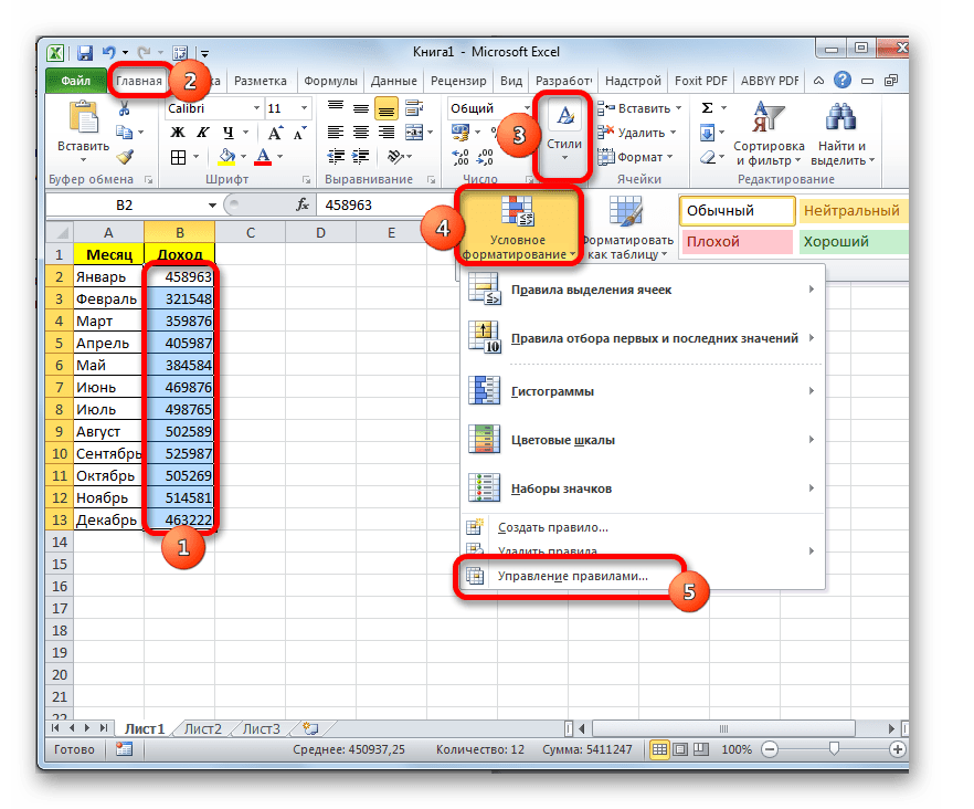
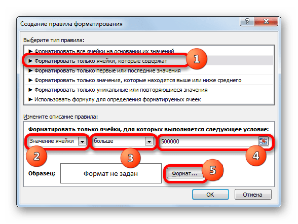
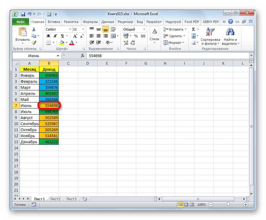
Посмотрим, как этот способ работает на конкретном примере. Имеем таблицу доходов предприятия, в которой данные разбиты помесячно. Нам нужно выделить разными цветами те элементы, в которых величина доходов менее 400000 рублей, от 400000 до 500000 рублей и превышает 500000 рублей.

Выделяем столбец, в котором находится информация по доходам предприятия. Затем перемещаемся во вкладку «Главная». Щелкаем по кнопке «Условное форматирование», которая располагается на ленте в блоке инструментов «Стили». В открывшемся списке выбираем пункт «Управления правилами…».

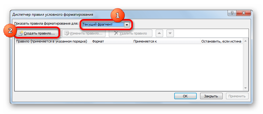
Запускается окошко управления правилами условного форматирования. В поле «Показать правила форматирования для» должно быть установлено значение «Текущий фрагмент». По умолчанию именно оно и должно быть там указано, но на всякий случай проверьте и в случае несоответствия измените настройки согласно вышеуказанным рекомендациям. После этого следует нажать на кнопку «Создать правило…».

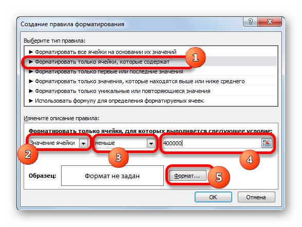
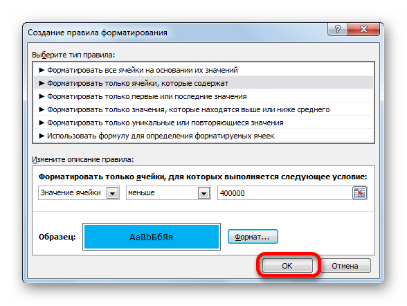
Открывается окно создания правила форматирования. В списке типов правил выбираем позицию «Форматировать только ячейки, которые содержат». В блоке описания правила в первом поле переключатель должен стоять в позиции «Значения». Во втором поле устанавливаем переключатель в позицию «Меньше». В третьем поле указываем значение, элементы листа, содержащие величину меньше которого, будут окрашены определенным цветом. В нашем случае это значение будет 400000. После этого жмем на кнопку «Формат…».

Открывается окно формата ячеек. Перемещаемся во вкладку «Заливка». Выбираем тот цвет заливки, которым желаем, чтобы выделялись ячейки, содержащие величину менее 400000. После этого жмем на кнопку «OK» в нижней части окна.

Возвращаемся в окно создания правила форматирования и там тоже жмем на кнопку «OK».

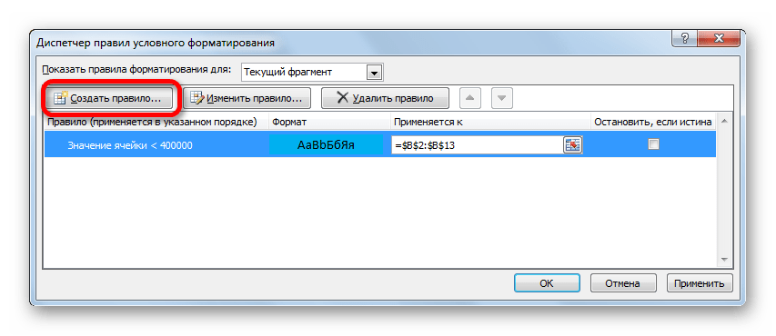
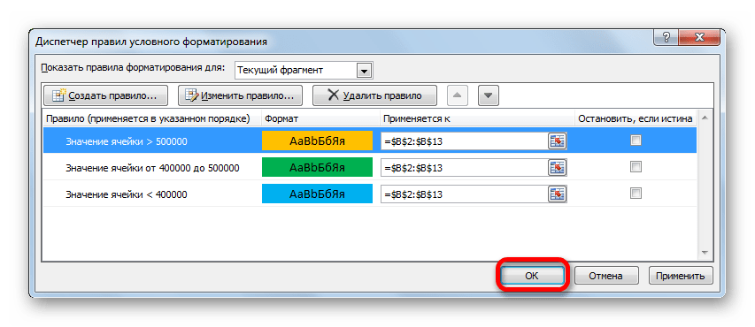
После этого действия мы снова будем перенаправлены в Диспетчер правил условного форматирования. Как видим, одно правило уже добавлено, но нам предстоит добавить ещё два. Поэтому снова жмем на кнопку «Создать правило…».

И опять мы попадаем в окно создания правила. Перемещаемся в раздел «Форматировать только ячейки, которые содержат». В первом поле данного раздела оставляем параметр «Значение ячейки», а во втором выставляем переключатель в позицию «Между». В третьем поле нужно указать начальное значение диапазона, в котором будут форматироваться элементы листа. В нашем случае это число 400000. В четвертом указываем конечное значение данного диапазона. Оно составит 500000. После этого щелкаем по кнопке «Формат…».

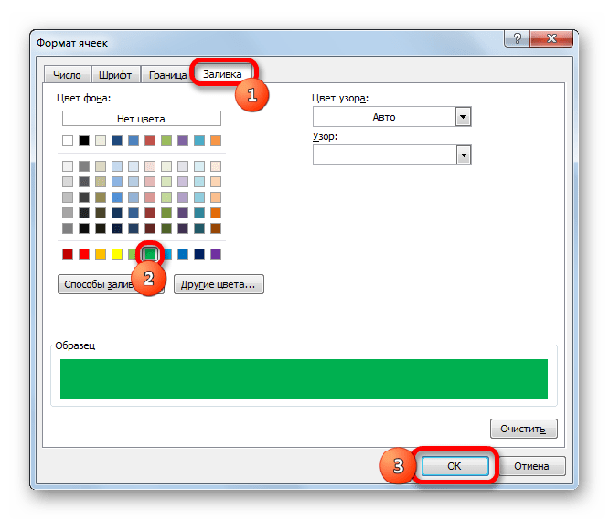
В окне форматирования снова перемещаемся во вкладку «Заливка», но на этот раз уже выбираем другой цвет, после чего жмем на кнопку «OK».

После возврата в окно создания правила тоже жмем на кнопку «OK».

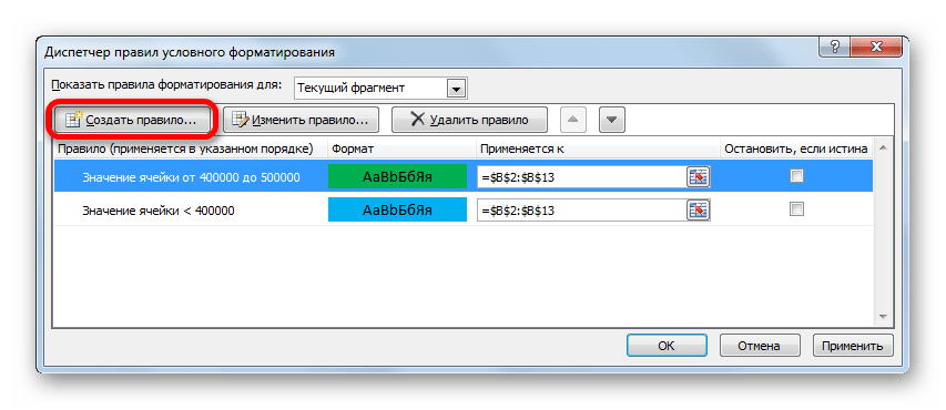
Как видим, в Диспетчере правил у нас создано уже два правила. Таким образом, осталось создать третье. Щелкаем по кнопке «Создать правило».

В окне создания правила опять перемещаемся в раздел «Форматировать только ячейки, которые содержат». В первом поле оставляем вариант «Значение ячейки». Во втором поле устанавливаем переключатель в полицию «Больше». В третьем поле вбиваем число 500000. Затем, как и в предыдущих случаях, жмем на кнопку «Формат…».

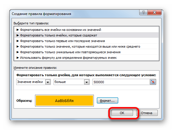
В окне «Формат ячеек» опять перемещаемся во вкладку «Заливка». На этот раз выбираем цвет, который отличается от двух предыдущих случаев. Выполняем щелчок по кнопке «OK».

В окне создания правил повторяем нажатие на кнопку «OK».

Открывается Диспетчер правил. Как видим, все три правила созданы, поэтому жмем на кнопку «OK».

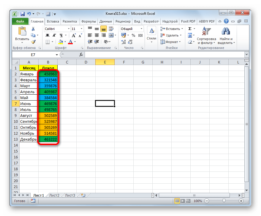
Теперь элементы таблицы окрашены согласно заданным условиям и границам в настройках условного форматирования.

Если мы изменим содержимое в одной из ячеек, выходя при этом за границы одного из заданных правил, то при этом данный элемент листа автоматически сменит цвет.

Кроме того, можно использовать условное форматирование несколько по-другому для окраски элементов листа цветом.

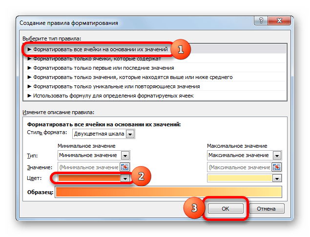
Для этого после того, как из Диспетчера правил мы переходим в окно создания форматирования, то остаемся в разделе «Форматировать все ячейки на основании их значений». В поле «Цвет» можно выбрать тот цвет, оттенками которого будут заливаться элементы листа. Затем следует нажать на кнопку «OK».

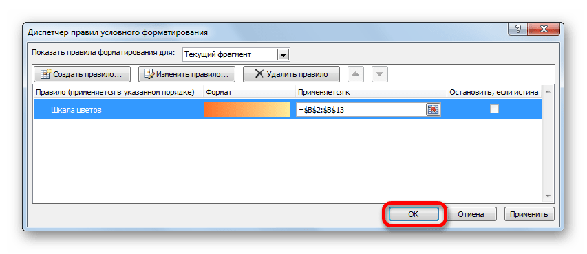
В Диспетчере правил тоже жмем на кнопку «OK».

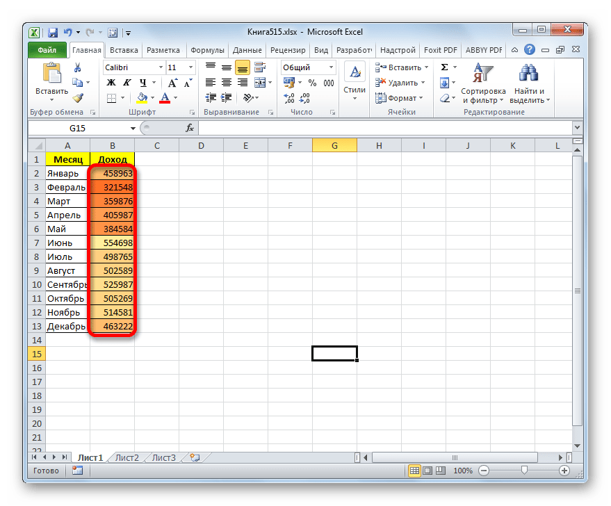
Как видим, после этого ячейки в колонке окрашиваются различными оттенками одного цвета. Чем значение, которое содержит элемент листа больше, тем оттенок светлее, чем меньше – тем темнее.

Урок: Условное форматирование в Экселе

Способ 2: использование инструмента «Найти и выделить»

Если в таблице находятся статические данные, которые не планируется со временем изменять, то можно воспользоваться инструментом для изменения цвета ячеек по их содержимому под названием «Найти и выделить». Указанный инструмент позволит отыскать заданные значения и изменить цвет в этих ячейках на нужный пользователю. Но следует учесть, что при изменении содержимого в элементах листа, цвет автоматически изменяться не будет, а останется прежним. Для того, чтобы сменить цвет на актуальный, придется повторять процедуру заново. Поэтому данный способ не является оптимальным для таблиц с динамическим содержимым.

Посмотрим, как это работает на конкретном примере, для которого возьмем все ту же таблицу дохода предприятия.

Выделяем столбец с данными, которые следует отформатировать цветом. Затем переходим во вкладку «Главная» и жмем на кнопку «Найти и выделить», которая размещена на ленте в блоке инструментов «Редактирование». В открывшемся списке кликаем по пункту «Найти».

Запускается окно «Найти и заменить» во вкладке «Найти». Прежде всего, найдем значения до 400000 рублей. Так как у нас нет ни одной ячейки, где содержалось бы значение менее 300000 рублей, то, по сути, нам нужно выделить все элементы, в которых содержатся числа в диапазоне от 300000 до 400000. К сожалению, прямо указать данный диапазон, как в случае применения условного форматирования, в данном способе нельзя.
Но существует возможность поступить несколько по-другому, что нам даст тот же результат. Можно в строке поиска задать следующий шаблон «3?????». Знак вопроса означает любой символ. Таким образом, программа будет искать все шестизначные числа, которые начинаются с цифры «3». То есть, в выдачу поиска попадут значения в диапазоне 300000 – 400000, что нам и требуется. Если бы в таблице были числа меньше 300000 или меньше 200000, то для каждого диапазона в сотню тысяч поиск пришлось бы производить отдельно.

Вводим выражение «3?????» в поле «Найти» и жмем на кнопку «Найти все».

После этого в нижней части окошка открываются результаты поисковой выдачи. Кликаем левой кнопкой мыши по любому из них. Затем набираем комбинацию клавиш Ctrl+A. После этого выделяются все результаты поисковой выдачи и одновременно выделяются элементы в столбце, на которые данные результаты ссылаются.

После того, как элементы в столбце выделены, не спешим закрывать окно «Найти и заменить». Находясь во вкладке «Главная» в которую мы переместились ранее, переходим на ленту к блоку инструментов «Шрифт». Кликаем по треугольнику справа от кнопки «Цвет заливки». Открывается выбор различных цветов заливки. Выбираем тот цвет, который мы желаем применить к элементам листа, содержащим величины менее 400000 рублей.

Как видим, все ячейки столбца, в которых находятся значения менее 400000 рублей, выделены выбранным цветом.

Теперь нам нужно окрасить элементы, в которых располагаются величины в диапазоне от 400000 до 500000 рублей. В этот диапазон входят числа, которые соответствуют шаблону «4??????». Вбиваем его в поле поиска и щелкаем по кнопке «Найти все», предварительно выделив нужный нам столбец.

Аналогично с предыдущим разом в поисковой выдаче производим выделение всего полученного результата нажатием комбинации горячих клавиш CTRL+A. После этого перемещаемся к значку выбора цвета заливки. Кликаем по нему и жмем на пиктограмму нужного нам оттенка, который будет окрашивать элементы листа, где находятся величины в диапазоне от 400000 до 500000.

Как видим, после этого действия все элементы таблицы с данными в интервале с 400000 по 500000 выделены выбранным цветом.

Теперь нам осталось выделить последний интервал величин – более 500000. Тут нам тоже повезло, так как все числа более 500000 находятся в интервале от 500000 до 600000. Поэтому в поле поиска вводим выражение «5?????» и жмем на кнопку «Найти все». Если бы были величины, превышающие 600000, то нам бы пришлось дополнительно производить поиск для выражения «6?????» и т.д.

Опять выделяем результаты поиска при помощи комбинации Ctrl+A. Далее, воспользовавшись кнопкой на ленте, выбираем новый цвет для заливки интервала, превышающего 500000 по той же аналогии, как мы это делали ранее.

Как видим, после этого действия все элементы столбца будут закрашены, согласно тому числовому значению, которое в них размещено. Теперь можно закрывать окно поиска, нажав стандартную кнопку закрытия в верхнем правом углу окна, так как нашу задачу можно считать решенной.

Но если мы заменим число на другое, выходящее за границы, которые установлены для конкретного цвета, то цвет не поменяется, как это было в предыдущем способе. Это свидетельствует о том, что данный вариант будет надежно работать только в тех таблицах, в которых данные не изменяются.

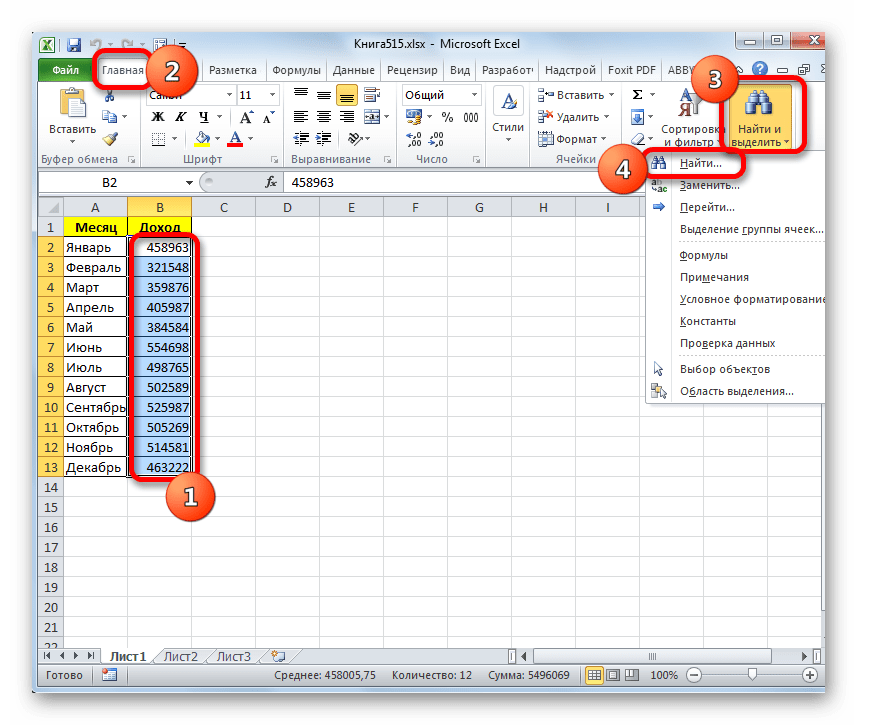
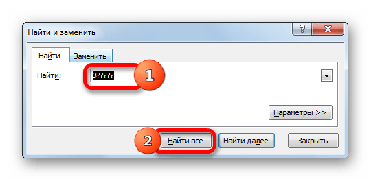
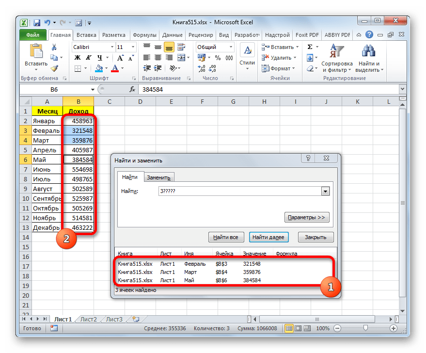
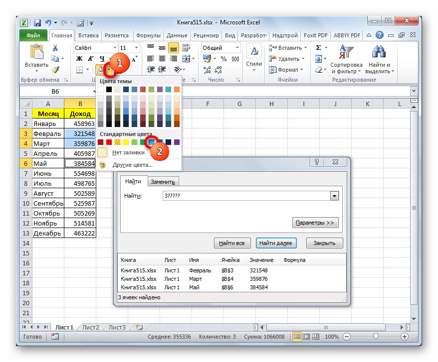
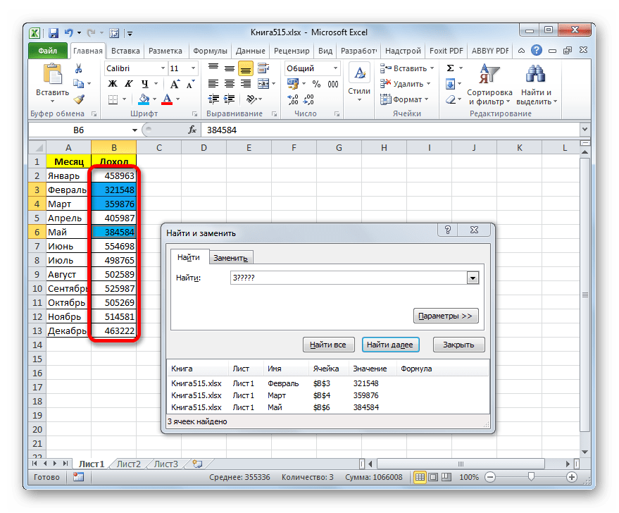
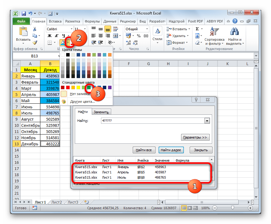
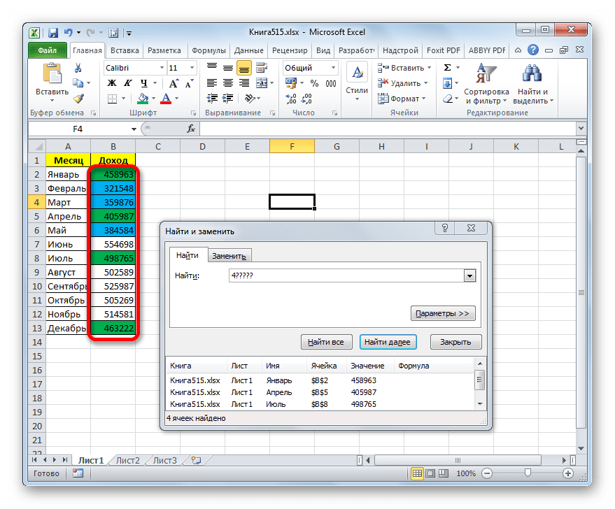
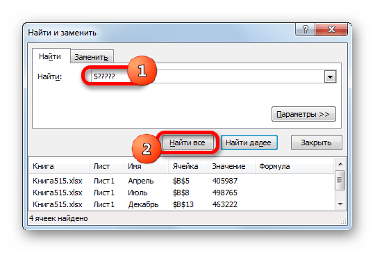
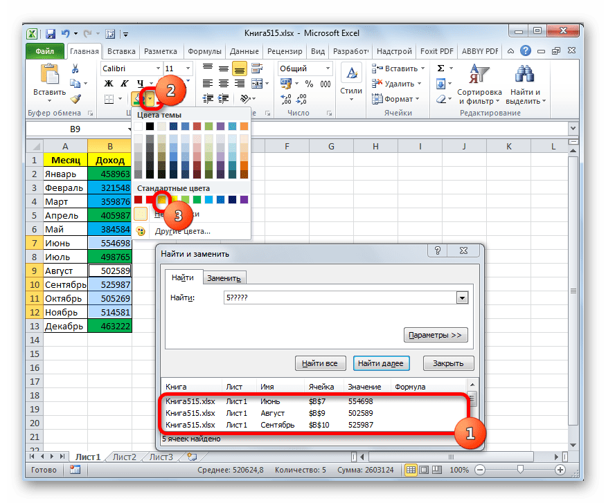
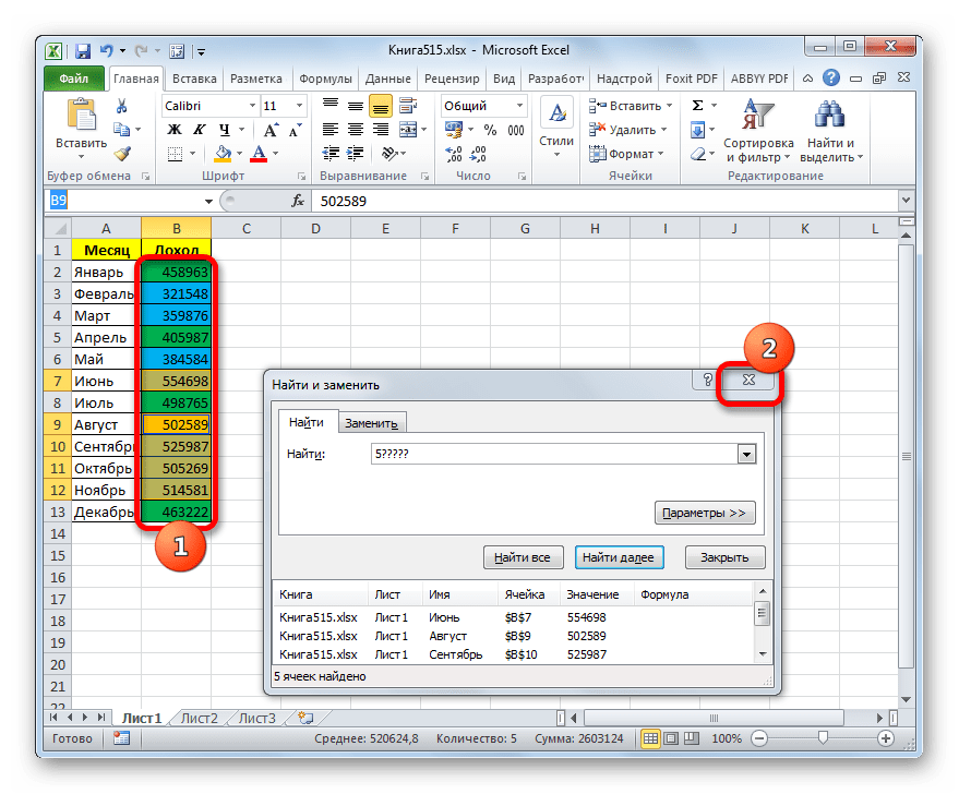
Урок: Как сделать поиск в Экселе

Как видим, существует два способа окрасить ячейки в зависимости от числовых значений, которые в них находятся: с помощью условного форматирования и с использованием инструмента «Найти и заменить». Первый способ более прогрессивный, так как позволяет более четко задать условия, по которым будут выделяться элементы листа. К тому же, при условном форматировании цвет элемента автоматически меняется, в случае изменения содержимого в ней, чего второй способ делать не может. Впрочем, заливку ячеек в зависимости от значения путем применения инструмента «Найти и заменить» тоже вполне можно использовать, но только в статических таблицах.

Источник

Let’s say that one of our tasks is to entering of the information about: did the ordering to a customer in the current month. Then on the basis of the information you need to select the cell in color according to the condition: which from customers have not made any orders for the past 3 months. For these customers you will need to re-send the offer.

Of course it’s the task for Excel. The program should automatically find such counterparties and, accordingly, to color ones. For these conditions we will use to the conditional formatting.

The filling cells with dates automatically

At first, you need to prepare to the structure for filling the register. First of all, let’s consider to the ready example of the automated register, which is depicted in the picture below. Today date 07.07.2018:

Today.

The user to need only to specify, if the customer have made an order in the current month, in the corresponding cell you should enter the text value of «order». The main condition for the allocation: if for 3 months the contractor did not make any order, his number is automatically highlighted in red.

Presented this decision should automate some work processes and to simplify to the visual data analysis.

The automatic filling of the cells with the relevant dates

At first, for the register with numbers of customers we will create to the column headers with green and up to date for months that will automatically display to the periods of time. To do this, in the cell B1 you need to enter the following formula:

DATE.

How does the formula work for automatically generating of the outgoing months?

In the picture, the formula returns the period of time passing since the date of writing this article: 17.09.2017. In the first argument in the function DATE is the nested formula that always returns the current year to today’s date thanks to the functions: YEAR and TODAY. In the second argument is the month number (-1). The negative number means that we are interested in what it was a month last time. The example of the conditions for the second argument with the value:

1 means the first month (January) in the year that is specified in the first argument;
0 – it is 1 month ago;
-1 – there is 2 months ago from the beginning of the current year (i.e. 01.10.2016).

The last argument-is the day number of the month, which is specified in the second argument. As a result, the DATE function collects all parameters into a single value and the formula returns to the corresponding date.

Next, go to the cell C1 and type the following formula:

MONTH.

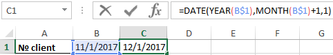
As you can see now the DATE function uses the value from the cell B1 and increases to the month number by 1 in relation to the previous cell. As the result is the 1 – the number of the following month.

Now you need to copy this formula from the cell C1 in the rest of the column headings in the range D1:AY1.

To highlight to the cell range B1:AY1 and select to the tool: «HOME»-«Cells»-«Format Cells» or just to press CTRL+1. In the dialog box that appears, in the tab «Number» in the section «Category» you need to select the option «Custom». In the «Type:» to enter the value: MMM. YY (required the letters in upper register). Because of this, we will get to the cropped display of the date values in the headers of the register, what simplifies to the visual analysis and make it more comfortable due to better readability.

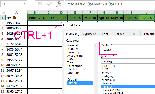
Please note! At the onset of the month of January (D1), the formula automatically changes in the date to the year in the next one.

How to select the column by color in Excel under the terms

Now you need to highlight to the cell by color which respect of the current month. Because of this, we can easily find the column in which you need to enter the actual data for this month. To do this:

To select the range of the cells B2:AY15 and select the tool: «HOME» -«Styles» -«Conditional Formatting»-«New Rule». And in the appeared window «New Formatting Rule» you need to select the option: «Use a formula to determine which cells to format»

In the input field to enter the formula:

Click «Format» and indicate on the tab «Fill» in what color (for example green) will be the selected cells of the current month. Then on all Windows for confirmation to click «OK».

Format.

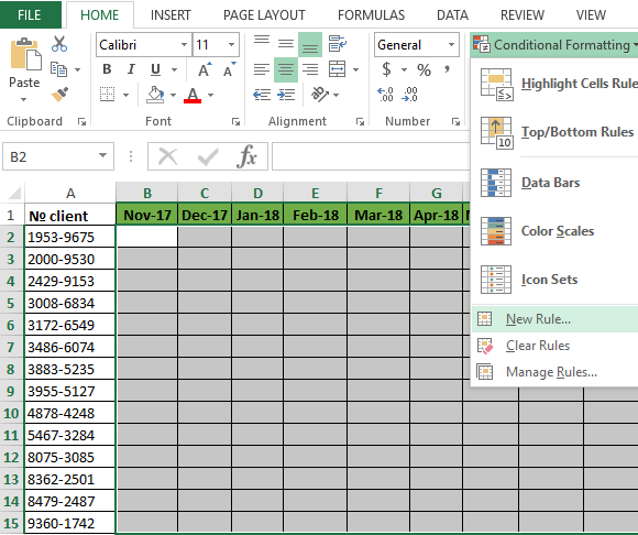
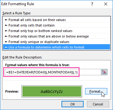
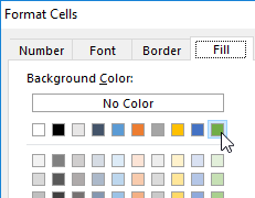
The column under the appropriate heading of the register is automatically highlighted in green accordingly to our terms and conditions:

How does the formula highlight of the column color on a condition work?

Due to the fact that before the creation of the conditional formatting rule we have covered all the table data for inputting data of register, the formatting will be active for each cell in the range B2:AY15. The mixed reference in the formula B$1 (absolute address only for rows, but for columns it is relative) determines that the formula will always to refer to the first row of each column.

Automatic highlighting of the column in the condition of the current month

The main condition for the fill by color of the cells: if the range B1:AY1 is the same date that the first day of the current month, then the cells in a column change its colors by specified in conditional formatting.

Please note! In this formula, for the last argument of the function DATE is shown 1, in the same way as for formulas in determining the dates for the column headings of the register.

In our case, is the green filling of the cells. If we open our register in next month, that it has the corresponding column is highlighted in green regardless of the current day.

The table is formatted, now we are filling it with the text value of the «order» in a mixed order of clients for current and past months.

How to highlight the cells in red color according to the condition

Now we need to highlight in red to the cells with the numbers of clients who for 3 months have not made any order. To do this:

Select the range of the cells A2:A15 (that is, the list of the customer numbers) and select to the tool: «HOME»-«Styles»-«Conditional formatting»-«Create rule». And in the window that appeared «Create a formatting rule» to select the option: «Use the formula for determining which cells to format».
This time in the input box to enter the formula:

To click «Format» and specify the red color on the tab «Fill». Then on all Windows click «OK».
Fill the cells with the text value of «order» as in the picture and look at the result:

result.

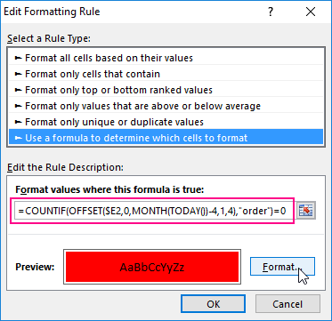
The numbers of customers are highlighted in red, if in the row has no have the value «order» in the last three cells for the current month (inclusively).

The analysis of the formula for the highlighting of cells according to the condition

Firstly, we will do by the middle part of our formula. The SHIFT function returns a range reference shifted relative to the basic range of the certain number of rows and columns. The returned reference can be a single cell or a range of cells. Optionally, you can define to the number of returned rows and columns. In our example, the function returns the reference to the cell range for the last 3 months.

The important part for our terms of highlighting in color – is belong to the first argument of the SHIFT function. It determines from which month to start the offset. In this example, there is the cell D2, that is, the beginning of the year – January. Of course for the rest of the cells in the column the row number for the base of the cell will correspond to the line number in what it is located. The following 2 arguments of the SHIFT function to determine how many rows and columns should be done offset. Since the calculations for each customer will carry in the same line, the offset value for the rows we specified is -0.

At the same time for the calculating the value of the third argument (the offset by the columns) we use to the nested formula MONTH(TODAY()), which in accordance with the terms returns to the number of the current month in the current year. From the calculated formula of the month as a number subtract the number 4, that is, in cases November we get the offset by 8 columns. And, for example, for June – there are on 2 columns only.

The last two arguments for the SHIFT function, determine the height (in the number of rows) and width (in the number of columns) of the returned range. In our example, there is the area of the cell with height on 1 row and with width on 4 columns. This range covers to the columns of 3 previous months and the current month.

The first function in the COUNTIF formula checks the condition: how many times in the returned range using the SHIFT function, we can found to the text value «order». If the function returns the value of 0, it means from the client with this number for 3 months there was not any order. And in accordance with our terms and conditions, the cell with number of this client is shown in red fill color.

If we want to register to data for customers, Excel is ideally suited for this purpose. You can easily record in the appropriate categories to the number of ordered goods, as well as the date of implementation of transaction. The problem gradually starts with arising of the data growth.

Download example automatic highlight cells by color.

If so many of them that we need to spend a few minutes looking for a specific position of the register and analysis of the information entered. In this case, it is necessary to add in the table to the register of mechanisms to automate some workflows of the user. And so we did.

Источник

When we work with a huge amount of data in Excel/Spreadsheet and need to highlight or color certain cells based on their values then it becomes very difficult to perform this task by changing the color of each cell one by one. Coloring the cells based on their values in Excel/Spreadsheet WPS(2016/2019/Mac/Online) helps in understanding the data and highlights the important data from the remaining cells.

Many people are unaware of How to Color Cell Based on Value in Excel/Spreadsheet

There are different ways for doing this task. After following the below-mentioned steps, anyone can easily color a cell based on value in Excel/Spreadsheet.

Excel/Spreadsheet is an easy-to-use tool that helps its users by providing so many different methods for processing and categorizing data within a few minutes. The following steps will help you understand How to color cell based on value in Excel/Spreadsheet WPS. After reading all the steps, you will be able to color cells based on value in excel/spreadsheet WPS (2016/2019/Mac/Online) easily.

1.Open the worksheet in Spreadsheets (WPS Office) which contains the desired data and select the data in which you want to color different cells.

2.Click on the Conditional Formatting button in the Home Tab. It will show different options, as shown below.

3.Select New Rule and then select Format only cells that contain.

4. Select the type of values that need to be colored. For example, in the below picture the values between 65 to 85 are required to be colored. After defining the values in the designated spaces, click on Format and a new window will open.

5.Go to Patterns tab and select your desired color and click on OK. This will color cells based on their values. The pictures below show all the steps in sequence.

How to Color Cell Based on Value of Another Cell in Excel/Spreadsheet

1.In case the color of cells is required to be changed based on the value of some specific cell then again select the data range.

2.Click on the Conditional Formatting button in the Home Tab. It will show different options. Select New Rule.

3.Now, select Format only cells that contain. Select less than in the drop-down menu and then select the specific cell by clicking on the button in the highlighted area.

4.Press Enter and then click on Format and select your desired color. Click on OK.

5.The color of cells will change based on the value of the specific cell. For example, look at the pictures below.

If you change the value of the specific cell, the cells will get colored as per the formatting rule selected earlier. This is shown below.

Note: You can repeat the same steps by selecting another formatting rule.

This article has covered the methods on How to color cells based on values in excel/spreadsheet WPS (2016/2019/Mac/Online) and how to color cells based on value of a specific cell in excel/spreadsheet WPS (2016/2019/Mac/Online). You can use these simple steps as explained above and easily color cells based on their values in your WPS Excel/Spreadsheet (2016/2019/Mac/Online) whenever required.

Learn More about How to Color Cells Based on Values in Excel/Spreadsheet

Hopefully, you have learned How to color cells based on values in WPS Excel/Spreadsheet (2016/2019/Mac/Online) by following the above steps. If you want to know more about Excel features, you can follow WPS Academy to learn. You can also download WPS Office to edit excel spreadsheets, word documents, and PowerPoint for free of cost. Download now! And get an easy and enjoyable working experience.

Источник

Based on certain values in our worksheet, we might decide to format the sheet by assigning colors based on values. In this tutorial, we will explore how to change color in excel based on values in Excel 2013, 2010 and 2016. We will also learn how to use Excel formulas to change the background colors of cells with formula errors or blank cells.

Figure 1 – How to change cell color based on the value

How to Change Cell Color Based On Value with Conditional Formatting

When we have a table and wish to change the color of certain cells dynamically, Excel conditional formatting is a great tool we can use. It will help us highlight the values less than Y, greater than X or between X and Y. To begin:

We will select the table or range where we want to change the background color of cells. Here we have selected the entire table.
Now, we will go to the Home tab, select styles group and choose Conditional formatting

Figure 2 – Formula for changing color

We will select New Rule and in the New Formatting Rule dialog box, under the Select a Rule type box, we can select any rule. For now, we will select “Format Only Cells that contain”.
In the lower part of the dialog box, where we have Format Only Cells with section, we will set the rule conditions. Next, we will choose to format only cells with a cell value between 90 and 140.

Figure 3 – New formatting rule dialog box

Now, we will click the Format button and choose the background color we want to apply
In the Format Cells dialog box, we will switch to the fill tab and pick the color we want. Next, we click OK.

Figure 4 – How to change font color based on the value

We will be redirected back to the New Formatting Rule window. Here, we will preview the format changes in the Preview box. Once we are satisfied with everything, we will click OK.

Figure 5 – How to change color

How to Change the Background Color for Special Cells (cells with formula errors or blanks)

In the Home tab, we will go to the Styles group and click Conditional formatting
Next, we will select New Rule. In the New Formatting Rule dialog, we will select the option Use a formula to determine which cells to format.
Now, we will enter one of the following formulas in the format values where this formula is true field. In our example, we will select the formula for changing the color of blank cells

=IsBlank() – to change the background color of blank cells.

=IsError() – to change the background color of cells with formulas that return errors.

Where () should contain the highlighted cells.

Figure 6 – Color cell based on the value of another cell

Alternatively, we can click on Format only Cells that contain and select Blanks in the lower end of the dialog box.

Figure 7 – Color cell based on the value of another cell

We will select the Format button and choose the background color we want in the fill Tab.

Figure 8 – How to change font color based on the value

In the Format Cells dialog box, we will switch to the fill tab and pick the color we want. Next, we will click OK.
We will be redirected back to the New Formatting Rule window. Here we will preview the format changes in the Preview box. Once we are satisfied with everything, we will click OK.

Figure 9 – How to excel change cell based on the value of another cell.

Instant Connection to an Excel Expert

Most of the time, the problem you will need to solve will be more complex than a simple application of a formula or function. If you want to save hours of research and frustration, try our live Excelchat service! Our Excel Experts are available 24/7 to answer any Excel question you may have. We guarantee a connection within 30 seconds and a customized solution within 20 minutes.

Источник

Need more help?

See Also

Процедура изменения цвета ячеек в зависимости от содержимого

Способ 1: условное форматирование

Способ 2: использование инструмента «Найти и выделить»

The filling cells with dates automatically

The automatic filling of the cells with the relevant dates

How does the formula work for automatically generating of the outgoing months?

How to select the column by color in Excel under the terms

How does the formula highlight of the column color on a condition work?

Automatic highlighting of the column in the condition of the current month

How to highlight the cells in red color according to the condition

The analysis of the formula for the highlighting of cells according to the condition

Many people are unaware of How to Color Cell Based on Value in Excel/Spreadsheet

How to Color Cell Based on Value of Another Cell in Excel/Spreadsheet

Learn More about How to Color Cells Based on Values in Excel/Spreadsheet

How to Change Cell Color Based On Value with Conditional Formatting

Instant Connection to an Excel Expert