
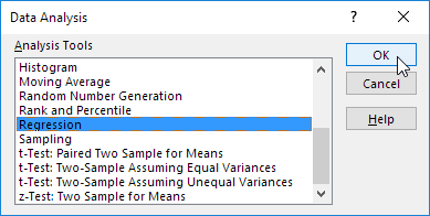
Click on the “Data” menu, and then choose the “Data Analysis” tab. You will now see a window listing the various statistical tests that Excel can perform. Scroll down to find the regression option and click “OK”.
Contents
- 1 How do you find the regression coefficient on Excel?
- 2 How do you find the regression coefficient?
- 3 What does coefficient mean in Excel regression?
- 4 How do you calculate residuals in Excel?
- 5 What is coefficient regression?
- 6 How is linear regression calculated?
- 7 How do you calculate linear regression by hand?
- 8 How do you do correlation and regression in Excel?
- 9 Is regression coefficient and correlation coefficient the same?
- 10 What is R2 in linear regression?
- 11 What is residual in Excel?
- 12 How do you do linear regression on Excel?
- 13 How do you do a regression in Excel with multiple variables?
- 14 What is a regression coefficient example?
- 15 What is regression and regression coefficient?
- 16 How many regression coefficients are there?
- 17 How do you solve regression analysis?
- 18 How do you find b1 and b0 in Excel?
- 19 How do you manually calculate correlation coefficient?
How do you find the regression coefficient on Excel?
Run regression analysis
- On the Data tab, in the Analysis group, click the Data Analysis button.
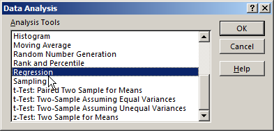
- Select Regression and click OK.
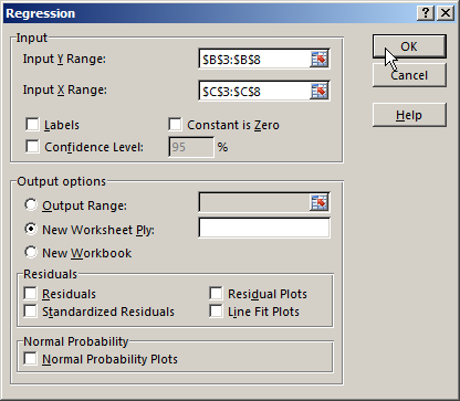
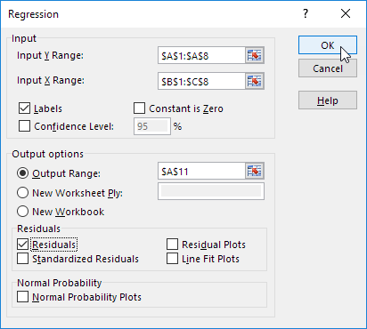
- In the Regression dialog box, configure the following settings: Select the Input Y Range, which is your dependent variable.
- Click OK and observe the regression analysis output created by Excel.
How do you find the regression coefficient?
A regression coefficient is the same thing as the slope of the line of the regression equation. The equation for the regression coefficient that you’ll find on the AP Statistics test is: B1 = b1 = Σ [ (xi – x)(yi – y) ] / Σ [ (xi – x)2]. “y” in this equation is the mean of y and “x” is the mean of x.
What does coefficient mean in Excel regression?
Coefficient: Gives you the least squares estimate. Standard Error: the least squares estimate of the standard error. T Statistic: The T Statistic for the null hypothesis vs.P Value: Gives you the p-value for the hypothesis test.
How do you calculate residuals in Excel?
Enter “=B1-C1” without quotes in cell D1 to calculate the residual, or the predicted value’s deviation from the actual amount.
Regression coefficients are estimates of the unknown population parameters and describe the relationship between a predictor variable and the response.The sign of each coefficient indicates the direction of the relationship between a predictor variable and the response variable.
How is linear regression calculated?
A linear regression line has an equation of the form Y = a + bX, where X is the explanatory variable and Y is the dependent variable. The slope of the line is b, and a is the intercept (the value of y when x = 0).
How do you calculate linear regression by hand?
Simple Linear Regression Math by Hand
- Calculate average of your X variable.
- Calculate the difference between each X and the average X.
- Square the differences and add it all up.
- Calculate average of your Y variable.
- Multiply the differences (of X and Y from their respective averages) and add them all together.
How do you do correlation and regression in Excel?
To use the Analysis Toolpak add-in in Excel to quickly generate correlation coefficients between multiple variables, execute the following steps.
- On the Data tab, in the Analysis group, click Data Analysis.
- Select Correlation and click OK.
- For example, select the range A1:C6 as the Input Range.
Is regression coefficient and correlation coefficient the same?
Correlation coefficient indicates the extent to which two variables move together. Regression indicates the impact of a change of unit on the estimated variable ( y) in the known variable (x). To find a numerical value expressing the relationship between variables.
What is R2 in linear regression?
R-squared is a goodness-of-fit measure for linear regression models. This statistic indicates the percentage of the variance in the dependent variable that the independent variables explain collectively.After fitting a linear regression model, you need to determine how well the model fits the data.
What is residual in Excel?
The residuals show you how far away the actual data points are fom the predicted data points (using the equation). For example, the first data point equals 8500.
How do you do linear regression on Excel?
To add a regression line, choose “Layout” from the “Chart Tools” menu. In the dialog box, select “Trendline” and then “Linear Trendline”. To add the R2 value, select “More Trendline Options” from the “Trendline menu.
How do you do a regression in Excel with multiple variables?
In Excel you go to Data tab, then click Data analysis, then scroll down and highlight Regression. In regression panel, you input a range of cells with Y data, with X data (multiple regressors), check the box with output range or new worksheet, and check all the plots that you need.
What is a regression coefficient example?
Coefficients are the numbers by which the variables in an equation are multiplied. For example, in the equation y = -3.6 + 5.0X 1 – 1.8X 2, the variables X 1 and X 2 are multiplied by 5.0 and -1.8, respectively, so the coefficients are 5.0 and -1.8. The coefficients are 2 and -3.
What is regression and regression coefficient?
The regression coefficients are a statically measure which is used to measure the average functional relationship between variables. In regression analysis, one variable is dependent and other is independent. Also, it measures the degree of dependence of one variable on the other(s).
How many regression coefficients are there?
With simple linear regression, there are only two regression coefficients – b0 and b1.
How do you solve regression analysis?
Regression analysis is the analysis of relationship between dependent and independent variable as it depicts how dependent variable will change when one or more independent variable changes due to factors, formula for calculating it is Y = a + bX + E, where Y is dependent variable, X is independent variable, a is
How do you find b1 and b0 in Excel?
Use [email protected] =LINEST(ArrayY, ArrayXs) to get b0, b1 and b2 simultaneously.
How do you manually calculate correlation coefficient?
Here are the steps to take in calculating the correlation coefficient:
- Determine your data sets.
- Calculate the standardized value for your x variables.
- Calculate the standardized value for your y variables.
- Multiply and find the sum.
- Divide the sum and determine the correlation coefficient.
Regression and correlation analysis – there are statistical methods. There are the most common ways to show the dependence of some parameter from one or more independent variables.
Lover on the specific practical examples, we consider these two are very popular analysis among economists. And give an example of the receiving the results when they are combined.
Regression analysis in Excel
It shows the influence of some values (independent, substantive ones) on the dependent variable. For example, it depends on the number of economically active population from the number of enterprises, the value of wages and other parameters. Or: how to influence foreign investment, energy prices, etc. on the level of GDP.
The analysis result allows you to prioritize. And based on the main factors you may to predict, to plan the development of priorities areas, to make to the management decisions.
Regression is:
- the linear (у = а + bx);
- the parabolic (y = a + bx + cx2);
- the exponential (y = a * exp(bx));
- the power (y = a*x^b);
- the hyperbolic (y = b/x + a);
- the logarithmic (y = b * 1n(x) + a);
- the exponential (y = a * b^x).
Consider the example to the construction of a regression model in Excel and the interpretation of the results. Consider the linear regression type.
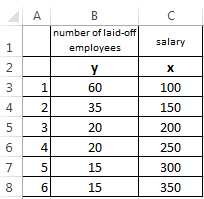
The task. On 6 enterprises was analyzed the average monthly salary and the number of employees who retired. It is necessary to determine the dependence of the number of employees who retired from the average salary.
The linear regression model is as follows:
У = а0 + а1х1 +…+акхк.
Where a – are the regression coefficients, x – the influencing variables, k – the number of factors.
In our example as Y serves the indicator of employees who retired. The influence factor – is the wage (x).
In Excel, there are built-in features with which you can calculate the parameters of the linear regression model. But faster it will make the add-on «analysis package».
Activate the powerful analytical tool:
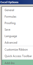
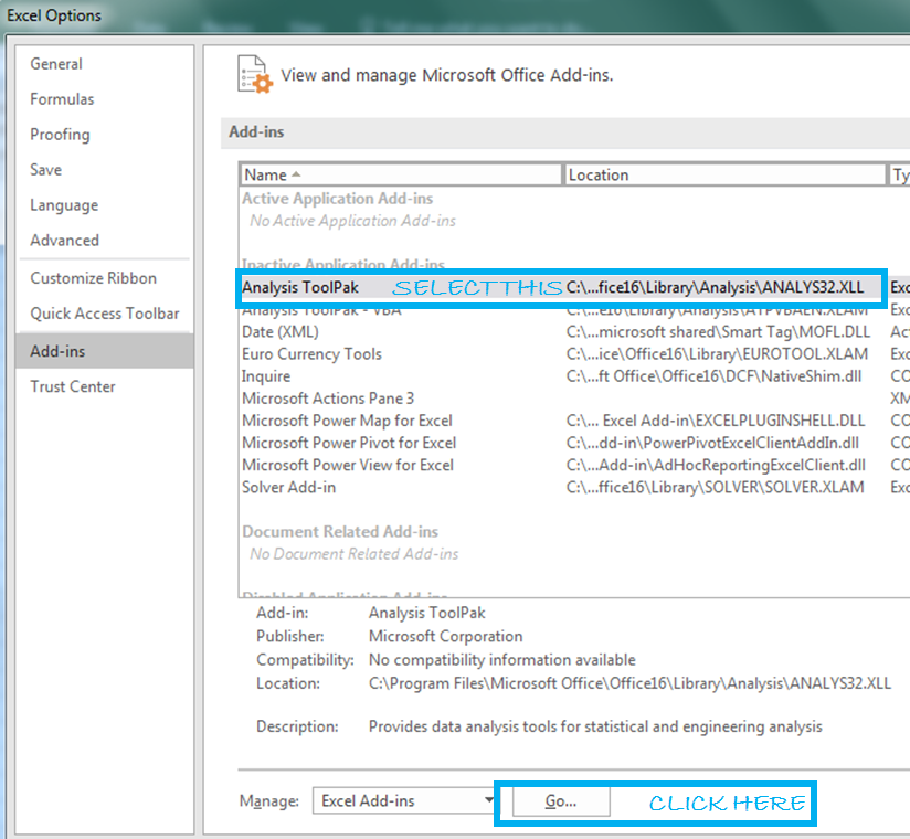
- Push the button «FILE»-«Options»-«Add-Ins».
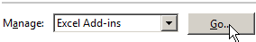
- Below the drop-down list in the «Manage:» field is the inscription «Excel Add-Ins» (if it is not, click on the checkbox to the right and select). And click the «Go» button. Hit.
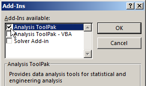
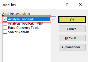
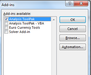
- The list of available add-ins. Select the «Analysis ToolPak» and click OK.
After activating the superstructure will be available on the «DATA» tab.
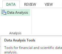
We direct regression analysis now.
- Open the «Data Analysis» tool menu. Select the «Regression».
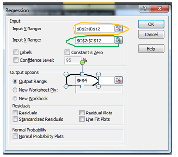
- Open the menu for selecting the input values and output parameters (which display the result). In the fields for the specify range of the input data, which describes the options (Y) and influence the factor (X). The rest can not fill.
- After you click OK, the program will display the calculations on a new page (you can choose the interval to be displayed on the current page or assign to the output to a new book).
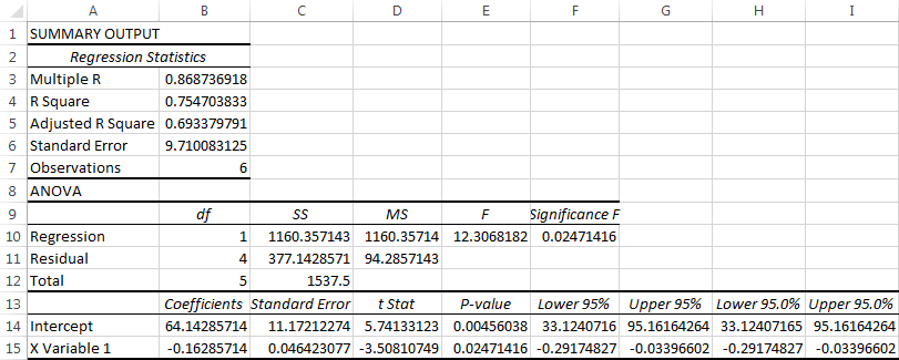
Firstly of all pay attention to the R-squared and the ratios.
R-square – is the coefficient of the determination. In our example – there is 0. 755, or 75. 5%. This means that the model parameters estimated at 75. 5% explains the addiction between the parameters whixh are studied. The higher the coefficient of determination, the better is the model. Good — above 0. 8. Bad — less than 0. 5 (such an analysis can hardly be considered reasonable). In our example – is «not bad».
64. 1428 ratio shows how will be Y, if all the variables in the model will be equal to 0. That is, the value of the analyzed parameter is influenced by other factors, which has not been described in the model.
-0. 16285 ratio shows the weight of the variable X to Y. That is, the average monthly salary in the range of the model affects the number of resignations from the weight -0. 16285 (this is a small effect). The sign «-» indicates to a negative effect: the higher the salary, the less dismissed. That is true.
Correlation analys in Excel
The correlation analysis helps to establish whether there is between the indices in one or two samples of the connection. For example, the time between the time machine and repair costs, equipment costs and operation duration, height and weight of children, etc.
If there is the connection is available, whether the increment of one the increase parameter (positive correlation) or the decreasing (negative) of the other one. The correlation analysis helps to the analyst to determine whether it is possible for the value of one indicator to predict the potential value of the other one.
The correlation coefficient is denoted by r. It ranges from +1 to -1. The classification of correlations for different areas will be different. If the value of the coefficient is 0 linear dependence between samples does not exist.
Consider how with helping Excel tools to find the correlation coefficient.
To find the paired coefficients applied CORREL function.
The task: To determine whether there is the interrelation between the operating time of the lathe and the costing of its maintenance.
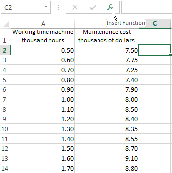
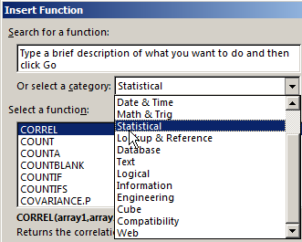
Put the cursor in any cell and click the fx button.
- In «Statistics» category select to the function =CORREL().
- The argument «Array 1» – is the first range of the values — while the machine: A2: A14.
- The argument «Array 2» – is the second range of values — the cost of repairs: B2: B14. Click OK.
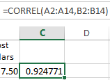
To determine the type of connection, it is necessary to see the absolute number of the coefficient (each a scale has for each field).
Note. For the correlation analysis of several parameters (more 2) it is more convenient to use the «Data Analysis» (add-on «Analysis Package»). In the list you need to choose and mark correlation array. That`s all. These coefficients are appeared in the correlation matrix.
The regression analysis
In practice, these two techniques are often used together.
The example:
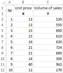
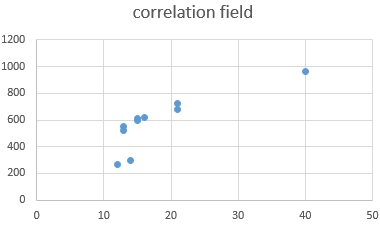
- Build to the correlation field: «INSERT» — «Charts» — «Scatter» (enables to compare pairs). The value range – there are all the numeric dates in the table.
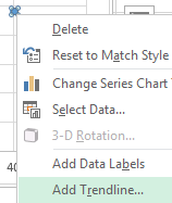
- Click with the left mouse button on any point on the chart. Then right. In the menu, select «Add Trendline».
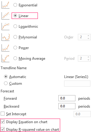
- Assign the parameters for the line. Type – is «Linear». Below – «Display equation on chart» and «Display R-squared value on chart».
Done:
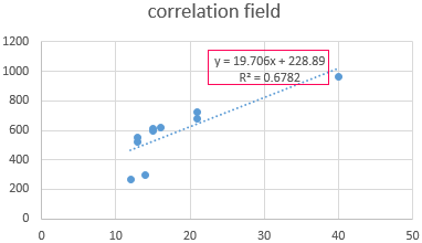
They are now visible and regression analysis dates.
Содержание
- Regression
- R Square
- Significance F and P-values
- Coefficients
- Residuals
- Linear Regression in Excel
- Excel Linear Regression
- How to Add Linear Regression Data Analysis Tool in Excel?
- Examples
- Things to Remember
- Recommended Articles
- Creating a Linear Regression Model in Excel
- What Is Linear Regression?
- Key Takeaways
- Important Considerations
- Outputting a Regression in Excel
- Interpret the Results
- Interpreting the Results
- Charting a Regression in Excel
- How Do You Interpret a Linear Regression?
- How Do You Know If a Regression Is Significant?
- How Do You Interpret the R-Squared of a Linear Regression?
Regression
This example teaches you how to run a linear regression analysis in Excel and how to interpret the Summary Output.
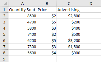
Below you can find our data. The big question is: is there a relation between Quantity Sold (Output) and Price and Advertising (Input). In other words: can we predict Quantity Sold if we know Price and Advertising?
1. On the Data tab, in the Analysis group, click Data Analysis.
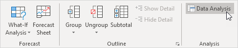
Note: can’t find the Data Analysis button? Click here to load the Analysis ToolPak add-in.
2. Select Regression and click OK.
3. Select the Y Range (A1:A8). This is the predictor variable (also called dependent variable).
4. Select the X Range(B1:C8). These are the explanatory variables (also called independent variables). These columns must be adjacent to each other.
6. Click in the Output Range box and select cell A11.
7. Check Residuals.
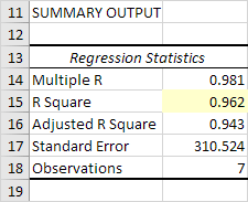
Excel produces the following Summary Output (rounded to 3 decimal places).
R Square
R Square equals 0.962 , which is a very good fit. 96% of the variation in Quantity Sold is explained by the independent variables Price and Advertising. The closer to 1, the better the regression line (read on) fits the data.
Significance F and P-values
To check if your results are reliable (statistically significant), look at Significance F ( 0.001 ). If this value is less than 0.05, you’re OK. If Significance F is greater than 0.05, it’s probably better to stop using this set of independent variables. Delete a variable with a high P-value (greater than 0.05) and rerun the regression until Significance F drops below 0.05.
Most or all P-values should be below below 0.05. In our example this is the case. ( 0.000 , 0.001 and 0.005 ).

Coefficients
The regression line is: y = Quantity Sold = 8536.214 -835.722 * Price + 0.592 * Advertising. In other words, for each unit increase in price, Quantity Sold decreases with 835.722 units. For each unit increase in Advertising, Quantity Sold increases with 0.592 units. This is valuable information.
You can also use these coefficients to do a forecast. For example, if price equals $4 and Advertising equals $3000, you might be able to achieve a Quantity Sold of 8536.214 -835.722 * 4 + 0.592 * 3000 = 6970.
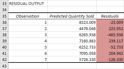
Residuals
The residuals show you how far away the actual data points are fom the predicted data points (using the equation). For example, the first data point equals 8500. Using the equation, the predicted data point equals 8536.214 -835.722 * 2 + 0.592 * 2800 = 8523.009, giving a residual of 8500 — 8523.009 = -23.009 .
You can also create a scatter plot of these residuals.
Источник
Linear Regression in Excel


Excel Linear Regression
Linear regression is a statistical tool in Excel used as a predictive analysis model to check the relationship between two sets of data or variables. We can estimate the relationship between two or more variables using this analysis. For example, we can see two variables: dependent and independent variables.
- The dependent variable is the factor we are trying to estimate.
- The independent variable is the factor that influences the dependent variable.
So, using Excel linear regression, we can see how the dependent variable goes through changes when the independent variable changes and helps us to decide which variable has a real impact mathematically.
Table of contents
You are free to use this image on your website, templates, etc., Please provide us with an attribution link How to Provide Attribution? Article Link to be Hyperlinked
For eg:
Source: Linear Regression in Excel (wallstreetmojo.com)
How to Add Linear Regression Data Analysis Tool in Excel?
This tool is not visible until the user enables this. To enable this, follow the below steps.
- We must first go to the FILES >>Options.

Then, click on “Add-ins” under “Excel Options.”
Select “Excel Add-ins” under the “Manage” dropdown list in Excel and click on “Go.”

Check the box “Analysis ToolPak” in the “Add-Ins.”
Now, we should see the ” Data Analysis” option under the “Data” tab.

With this option, we can conduct many “Data Analysis” options. Let us see some of the examples now.
Examples
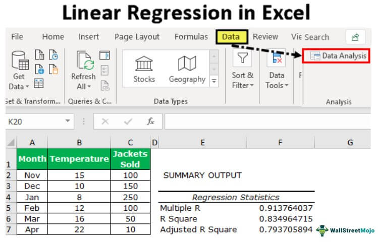
As we told you, linear regression Excel consists of two things: dependent and independent variables. For this example, we will use the below data of winter season jacket sold data with temperature in each month.
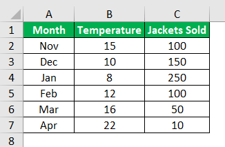
We have each month’s average temperature and jacket sold data. Here, we need to know which independent and dependent variables are.
Here “Temperature” is the independent variable because one cannot control the temperature, so this is the independent variable.
“Jackets Sold” is the dependent variable because the temperature increases and decreases in jacket sales.
Now, we will do the Excel linear regression analysis for this data.
- Step 1: We must click on the “Data” tab and “Data Analysis.”
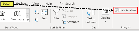
- Step 2: Once we click on “Data Analysis,” we will see the below window. Scroll down and select “Regression” in excel.

- Step 3: Select the “Regression” option and click on “OK” to open the window below.
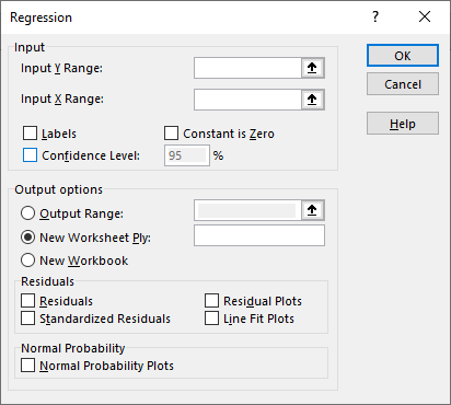
- Step 4: Here, the “Input Y Range” is the dependent variable, so in this case, our dependent variable is “Jackets Sold” data.
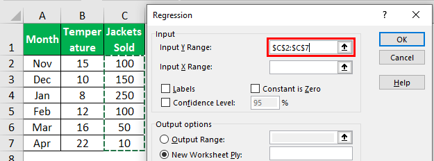
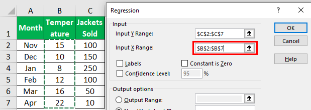
- Step 5: The “Input X Range” is the independent variable, so in this case, our independent variable is “Temperature” data.
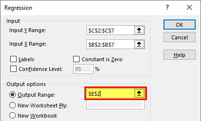
- Step 6: Select the output range as one of the cells.
- Step 7: To get the difference between the predicted and actual values, check the “Residuals” box.
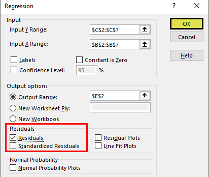
- Step 8: Click on the “OK.” We will have the below analysis.

The first part of the analysis is “Regression Statistics.”
- 1 Indicates a strong positive relationship.
- -1 indicates a strong negative relationship.
- 0 indicates no relationship.
Things to Remember
- We can also use the LINEST function in excelLINEST Function In ExcelThe built-in LINEST Function in Excel calculates statistics for a line by the least-squares regression method & returns an array that defines the line proving to be well-suited for the given data.read more .
- We need to have a strong knowledge of statistics to interpret the data.
- If the data analysis is not visible under the “Data” tab, we need to enable this option under the “Add-ins” option.
Recommended Articles
This article is a guide to Linear Regression in Excel. We discuss linear regression data analysis in Excel, examples, and a downloadable Excel template. You may also look at these useful functions in Excel: –
Источник
Creating a Linear Regression Model in Excel
Graph the relationship between two variables
:max_bytes(150000):strip_icc()/troypic__troy_segal-5bfc2629c9e77c005142f6d9.jpg)
:max_bytes(150000):strip_icc()/InvestopediaHeadShot-988693bb87b54bb095bd3789cd117a50.jpg)
What Is Linear Regression?
Linear regression is a type of data analysis that considers the linear relationship between a dependent variable and one or more independent variables. It is typically used to visually show the strength of the relationship or correlation between various factors and the dispersion of results – all for the purpose of explaining the behavior of the dependent variable. The goal of a linear regression model is to estimate the magnitude of a relationship between variables and whether or not it is statistically significant.
Say we wanted to test the strength of the relationship between the amount of ice cream eaten and obesity. We would take the independent variable, the amount of ice cream, and relate it to the dependent variable, obesity, to see if there was a relationship. Given a regression is a graphical display of this relationship, the lower the variability in the data, the stronger the relationship and the tighter the fit to the regression line.
In finance, linear regression is used to determine relationships between asset prices and economic data across a range of applications. For instance, it is used to determine the factor weights in the Fama-French Model and is the basis for determining the Beta of a stock in the capital asset pricing model (CAPM).
Here, we look at how to use data imported into Microsoft Excel to perform a linear regression and how to interpret the results.
Key Takeaways
- Linear regression models the relationship between a dependent and independent variable(s).
- Also known as ordinary least squares (OLS), a linear regression essentially estimates a line of best fit among all variables in the model.
- Regression analysis can be considered robust if the variables are independent, there is no heteroscedasticity, and the error terms of variables are not correlated.
- Modeling linear regression in Excel is easier with the Data Analysis ToolPak.
- Regression output can be interpreted for both the size and strength of a correlation among one or more variables on the dependent variable.
Important Considerations
There are a few critical assumptions about your data set that must be true to proceed with a regression analysis. Otherwise, the results will be interpreted incorrectly or they will exhibit bias:
- The variables must be truly independent (using a Chi-square test).
- The data must not have different error variances (this is called heteroskedasticity (also spelled heteroscedasticity)).
- The error terms of each variable must be uncorrelated. If not, it means the variables are serially correlated.
If those three points sound complicated, they can be. But the effect of one of those considerations not being true is a biased estimate. Essentially, you would misstate the relationship you are measuring.
Outputting a Regression in Excel
The first step in running regression analysis in Excel is to double-check that the free Excel plugin Data Analysis ToolPak is installed. This plugin makes calculating a range of statistics very easy. It is not required to chart a linear regression line, but it makes creating statistics tables simpler. To verify if installed, select «Data» from the toolbar. If «Data Analysis» is an option, the feature is installed and ready to use. If not installed, you can request this option by clicking on the Office button and selecting «Excel options».
Using the Data Analysis ToolPak, creating a regression output is just a few clicks.
The independent variable in Excel goes in the X range.
Given the S&P 500 returns, say we want to know if we can estimate the strength and relationship of Visa (V) stock returns. The Visa (V) stock returns data populates column 1 as the dependent variable. S&P 500 returns data populates column 2 as the independent variable.
- Select «Data» from the toolbar. The «Data» menu displays.
- Select «Data Analysis». The Data Analysis — Analysis Tools dialog box displays.
- From the menu, select «Regression» and click «OK».
- In the Regression dialog box, click the «Input Y Range» box and select the dependent variable data (Visa (V) stock returns).
- Click the «Input X Range» box and select the independent variable data (S&P 500 returns).
- Click «OK» to run the results.
[Note: If the table seems small, right-click the image and open in new tab for higher resolution.]
Interpret the Results
Using that data (the same from our R-squared article), we get the following table:
The R 2 value, also known as the coefficient of determination, measures the proportion of variation in the dependent variable explained by the independent variable or how well the regression model fits the data. The R 2 value ranges from 0 to 1, and a higher value indicates a better fit. The p-value, or probability value, also ranges from 0 to 1 and indicates if the test is significant. In contrast to the R 2 value, a smaller p-value is favorable as it indicates a correlation between the dependent and independent variables.
Interpreting the Results
The bottom line here is that changes in Visa stock seem to be highly correlated with the S&P 500.
- In the regression output above, we can see that for every 1-point change in Visa, there is a corresponding 1.36-point change in the S&P 500.
- We can also see that the p-value is very small (0.000036), which also corresponds to a very large T-test. This indicates that this finding is highly statistically significant, so the odds that this result was caused by chance are exceedingly low.
- From the R-squared, we can see that the V price alone can explain more than 62% of the observed fluctuations in the S&P 500 index.
However, an analyst at this point may heed a bit of caution for the following reasons:
- With only one variable in the model, it is unclear whether V affects the S&P 500 prices, if the S&P 500 affects V prices, or if some unobserved third variable affects both prices.
- Visa is a component of the S&P 500, so there could be a co-correlation between the variables here.
- There are only 20 observations, which may not be enough to make a good inference.
- The data is a time series, so there could also be autocorrelation.
- The time period under study may not be representative of other time periods.
Charting a Regression in Excel
We can chart a regression in Excel by highlighting the data and charting it as a scatter plot. To add a regression line, choose «Add Chart Element» from the «Chart Design» menu. In the dialog box, select «Trendline» and then «Linear Trendline». To add the R 2 value, select «More Trendline Options» from the «Trendline menu. Lastly, select «Display R-squared value on chart». The visual result sums up the strength of the relationship, albeit at the expense of not providing as much detail as the table above.
:max_bytes(150000):strip_icc()/dotdash_Final_Creating_a_Linear_Regression_Model_in_Excel_Sep_2020-01-13cd503cc6e244c48ea436c71ebec7ec.jpg)
How Do You Interpret a Linear Regression?
The output of a regression model will produce various numerical results. The coefficients (or betas) tell you the association between an independent variable and the dependent variable, holding everything else constant. If the coefficient is, say, +0.12, it tells you that every 1-point change in that variable corresponds with a 0.12 change in the dependent variable in the same direction. If it were instead -3.00, it would mean a 1-point change in the explanatory variable results in a 3x change in the dependent variable, in the opposite direction.
How Do You Know If a Regression Is Significant?
In addition to producing beta coefficients, a regression output will also indicate tests of statistical significance based on the standard error of each coefficient (such as the p-value and confidence intervals). Often, analysts use a p-value of 0.05 or less to indicate significance; if the p-value is greater, then you cannot rule out chance or randomness for the resultant beta coefficient. Other tests of significance in a regression model can be t-tests for each variable, as well as an F-statistic or chi-square for the joint significance of all variables in the model together.
How Do You Interpret the R-Squared of a Linear Regression?
R 2 (R-squared) is a statistical measure of the goodness of fit of a linear regression model (from 0.00 to 1.00), also known as the coefficient of determination. In general, the higher the R 2 , the better the model’s fit. The R-squared can also be interpreted as how much of the variation in the dependent variable is explained by the independent (explanatory) variables in the model. Thus, an R-square of 0.50 suggests that half of all of the variation observed in the dependent variable can be explained by the dependent variable(s).
Источник
Multiple linear regression is one of the most commonly used techniques in all of statistics.
This tutorial explains how to interpret every value in the output of a multiple linear regression model in Excel.
Example: Interpreting Regression Output in Excel
Suppose we want to know if the number of hours spent studying and the number of prep exams taken affects the score that a student receives on a certain college entrance exam.
To explore this relationship, we can perform multiple linear regression using hours studied and prep exams taken as predictor variables and exam score as a response variable.
The following screenshot shows the regression output of this model in Excel:

Here is how to interpret the most important values in the output:
Multiple R: 0.857. This represents the multiple correlation between the response variable and the two predictor variables.
R Square: 0.734. This is known as the coefficient of determination. It is the proportion of the variance in the response variable that can be explained by the explanatory variables. In this example, 73.4% of the variation in the exam scores can be explained by the number of hours studied and the number of prep exams taken.
Adjusted R Square: 0.703. This represents the R Square value, adjusted for the number of predictor variables in the model. This value will also be less than the value for R Square and penalizes models that use too many predictor variables in the model.
Standard error: 5.366. This is the average distance that the observed values fall from the regression line. In this example, the observed values fall an average of 5.366 units from the regression line.
Observations: 20. The total sample size of the dataset used to produce the regression model.
F: 23.46. This is the overall F statistic for the regression model, calculated as regression MS / residual MS.
Significance F: 0.0000. This is the p-value associated with the overall F statistic. It tells us whether or not the regression model as a whole is statistically significant.
In this case the p-value is less than 0.05, which indicates that the explanatory variables hours studied and prep exams taken combined have a statistically significant association with exam score.
Coefficients: The coefficients for each explanatory variable tell us the average expected change in the response variable, assuming the other explanatory variable remains constant.
For example, for each additional hour spent studying, the average exam score is expected to increase by 5.56, assuming that prep exams taken remains constant.
We interpret the coefficient for the intercept to mean that the expected exam score for a student who studies zero hours and takes zero prep exams is 67.67.
P-values. The individual p-values tell us whether or not each explanatory variable is statistically significant. We can see that hours studied is statistically significant (p = 0.00) while prep exams taken (p = 0.52) is not statistically significant at α = 0.05.
How to Write the Estimated Regression Equation
We can use the coefficients from the output of the model to create the following estimated regression equation:
Exam score = 67.67 + 5.56*(hours) – 0.60*(prep exams)
We can use this estimated regression equation to calculate the expected exam score for a student, based on the number of hours they study and the number of prep exams they take.
For example, a student who studies for three hours and takes one prep exam is expected to receive a score of 83.75:
Exam score = 67.67 + 5.56*(3) – 0.60*(1) = 83.75
Keep in mind that because prep exams taken was not statistically significant (p = 0.52), we may decide to remove it because it doesn’t add any improvement to the overall model.
In this case, we could perform simple linear regression using only hours studied as the explanatory variable.
Additional Resources
Introduction to Simple Linear Regression
Introduction to Multiple Linear Regression
Regression is an Analysis Tool, which we use for analyzing large amounts of data and making forecasts and predictions in Microsoft Excel.
Want to predict the future? No, we are not going to learn astrology. We are into numbers and we will learn regression analysis in Excel today.
To predict future estimates, we will study:
- REGRESSION ANALYSIS USING EXCEL FUNCTIONS (MANUAL REGRESSION FINDING)
- REGRESSION ANALYSIS USING EXCEL’S ANALYSIS TOOLPAK ADD-IN
- REGRESSION CHART IN EXCEL
Let’s do it…
Scenario:
Let’s assume you sell soft drinks. How cool will it be if you can predict:
- How many soft drinks will be sold next year based on previous year’s data?
- Which fields need to be focused?
- And how can you increase your sales by changing your strategy?
It will be profitably awesome. Right?… I know. So let’s get started.
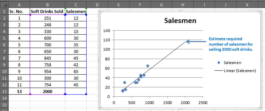
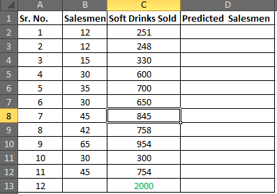
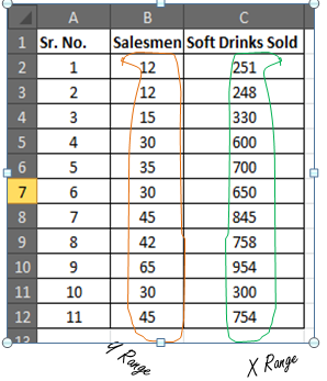
You have 11 records of salesmen and soft drinks sold.
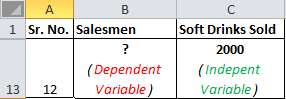
Now based on this data you want to predict the number of salesmen required to achieve 2000 sales of soft drinks.

The regression equation is a tool to make such close estimates. To do so, we need to know Regression first.
REGRESSION ANALYSIS USING EXCEL FUNCTIONS (MANUAL REGRESSION FINDING)
This part will make you understand regression better than just telling excel regression procedure.
Introduction:
Simple Linear Regression:
The study of the relationship between two variables is called Simple Linear Regression. Where one variable depends on the other independent variable. The dependent variable is often called by names such as Driven, Response, and Target variable. And the independent variable is often pronounced as a Driving, Predictor or simply Independent variable. These names clearly describe them.

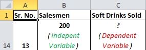
Now let’s compare this with your scenario. You want to know the number of salesmen required to achieve 2000 sales. So here, the dependent variable is the number of salesmen and the independent variable is sold soft drinks.
The independent variable is mostly denoted as x and dependent variable as y.
In our case, soft drinks are sold x and the number of salesmen is y.
If we want to know how many soft drinks will be sold if we appoint 200 salesmen, then the scenario will be vice-versa.
Moving On.
The “Simple” Math of Linear Regression Equation:
Well, it’s not simple. But Excel made it simple to do.
We need to predict the required number of salesmen for all 11 cases to get the 12th closest prediction.
Let’s say:
Soft Drink Sold is x
The number of Salesmen is y
The predicted y (number of salesmen) also called Regression Equation, would be
Now you must be wondering where the stat will you get the slope and intercept. Don’t worry, excel has functions for them. You do not need to learn how to find the slope and intercept it manually.
If you want, I will prepare a separate tutorial for that. Let me know in the comments section. These are some important data analytics tools.
Now let’s step into our calculation:
Step1: Prepare this small table
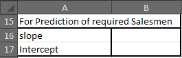
Step 2: Find the slope of the regression line
Excel Function for slopes is
=SLOPE(known_y’s,known_x’s)
Your known_y’s are in range B2:B12 and known_x’s are in range C2:C12

In cell B16, write the formula below
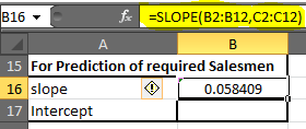
(Note: Slope is also called coefficient of x in the regression equation)
You will get 0.058409. Round up to 2 decimal digits and you will get 0.06.
Step 3: Find the Intercept of Regression Line
Excel function for the intercept is
=INTERCEPT(known_y’s, known_x’s)
We know what our known x’s and y’s
In cell B17, write down this formula

=INTERCEPT(B2:B12, C2:C12)
You will get a value of -1.1118969. Roundup to 2 decimal digits. You will get -1.11.
Our Linear Regression Equation is = x*0.06 + (-1.11). Now we can predict possible y depending on the target x easily.
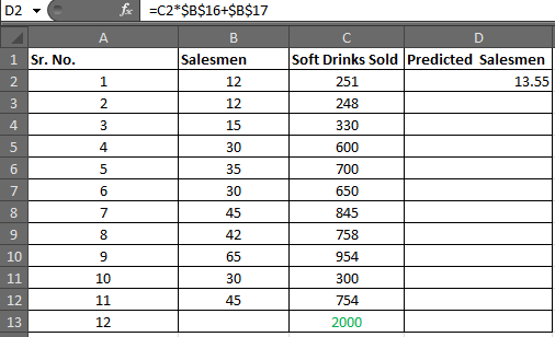
Step 4: In D2 write the formula below
=C2*$B$16+$B$17 (Regression Equation)
You will get a value of 13.55.
Select D2 to D13 and press CTRL+D to fill down the formula in the range D2:D13
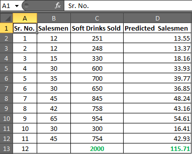
In cell D13 you have your required number of salesmen.
Hence, to achieve the target of 2000 Soft Drink Sales, you need an estimate of 115.71 salesmen or say 116 since it is illegal to cut humans into pieces.
Now using this you can easily conduct What-If analysis in excel. Just change the number of sales and it will show you many salesmen will it take to get that sales target achieved.
Play around it to find out:
How much workforce do you need to increase sales?
How many sales will increase if you increase your salesmen?
Make Your Estimate More Reliable:
Now you know that you need 116 salesmen to get 2000 sales done.
In analytics, nothing is just said and believed. You must give a percentage of reliability on your estimate. It is like giving a certificate of your equation.

Correlation Coefficient Formula:
The next thing you will be asked is how much these two variables are related. In static terms, you need to tell the coefficient of correlation.
Excel function for correlation is
In your case, known_x’s and Know_y’s are array1 and array2 irrespectively.
In B18 enter this formula
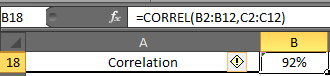
You will have 0.919090. Formate cell B2 into the percentage. Now have 92% of correlation.
Now, what this 92% means. It means, there 92% of chances of sales increase if you increase the number of salesmen and 92% of sales decrease if you decrease the number of salesmen. It is called Positive Correlation Coefficient.
R Squire (R^2) :
R Squire value tells you, by what percentage your regression equation is not a fluke. How much it is accurate by the data provided.
The Excel function for R squire is RSQ.
RSQ(known_y’s, Known_x’s)
In our case, we will get R squire value in cell B19.
In B19 enter this formula

So we have 84% of r Square value. Which is a very good explanation of our regression. It says that 84% of our data is just not by chance. Y (number of salesmen) is very much dependent on X (sales of soft drinks).
There are many other tests we can do on this data to ensure our regression. But manually it will be a complex and lengthy procedure. That is why excel provides Analysis Toolpak. Using this tool we can do this regression analysis in seconds.
REGRESSION IN EXCEL USING EXCEL’S ANALYSIS TOOLPAK ADD-IN
If you already know what regression equations are, and you just want your results quickly then this part is for you. But if you want to understand regression equations easily then scroll up to REGRESSION ANALYSIS USING EXCEL FUNCTIONS (MANUAL REGRESSION FINDING).
Excel provides a whole bunch of tools for analysis in its Analysis Toolpak. By default, it is not available in the Data tab. You need to add it. So let’s add it first.
Adding Analysis Toolpak to Excel 2016
If you don’t know where is data analysis in excel follow these steps
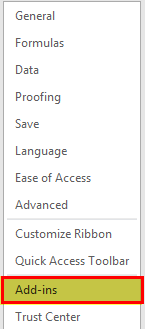
Step 1: Go to Excel Options: File? Options? Add-Ins
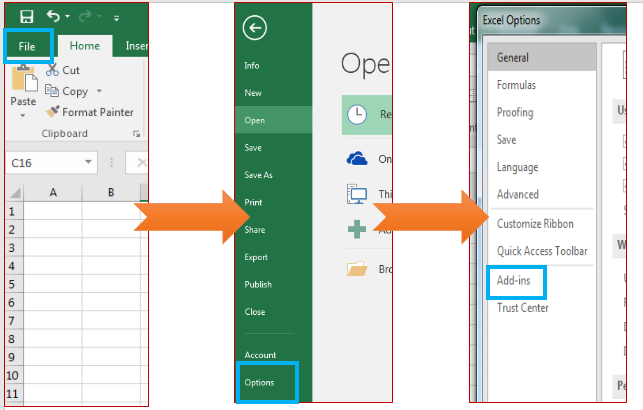
Step 2: Click on Add-Ins. You will see a list of available add-Ins.
Select Analysis ToolPak and at the bottom of the window, find manage. In manage select Excel Add-Ins and Click on GO.
Add-ins window will open. Here, select Analysis ToolPak. Then click the ok button.
Now you can access all functions of data analysis ToolPak from Data Tab.
Using Analysis ToolPak for Regression
Step 1: Go to the Data tab, Locate Data Analysis. Then click on it.

A dialogue box will pop up.
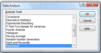
Step 2: Find ‘Regression’ in Analysis Tools list and hit the OK button.
The regression input window will pop up. You will see a number of available input options. But for now, we will just concentrate on Y Range and X Range, leaving everything else to default.

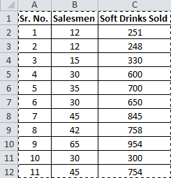
Step 4: Provide Inputs:
No. of Salesmen is Y
Sales of soft drinks are X
Hence
- Y Range= B2:B11
And
- X Range = C2:C11
For the output range, I have selected E4 on the same sheet. You may select a new worksheet to get results on a new worksheet in the same workbook or a complete new workbook. When you are done with your inputs, hit the OK button.
Results:
You will be served with a variety of information from your data. Don’t get overwhelmed. You don’t need to consume all the dishes.
We will only deal with those results which will help us to estimate the required number of salesmen
Step 5: We know the regression equation for estimation of y, that is
x*Slope+Intercept
We just need to locate Slope and Intercept in results.
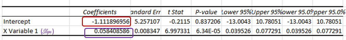
And here they are.
The intercept Coefficient is clearly mentioned.
The slope is written as ‘X Variable 1’, some times also mentioned as the coefficient of X. Round up them and we will get -1.11 as Intercept and 0.06 as Slope.
Step 6: From results, we can drive the Regression equation. And that would be
=x*(0.06) + (-1.11)
Prepare this table in excel.

For now, x is 2000, which is in cell E2.
In Cell F2 enter this formula
=E2*F21+F20
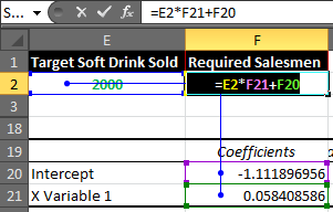
You will get a result of 115.7052757.

Rounding it up will give us 116 of Required Salesmen.
So we have learned how to form the regression equation manually and using Analysis ToolPak. How can you use this equation to estimate future stats?
Now let’s understand the regression output given by Analysis Toolpak.
Understanding the Regression Output:
There is no benefit, if you do regression analysis using analysis tool pack in excel and can’t interpret its meaning.
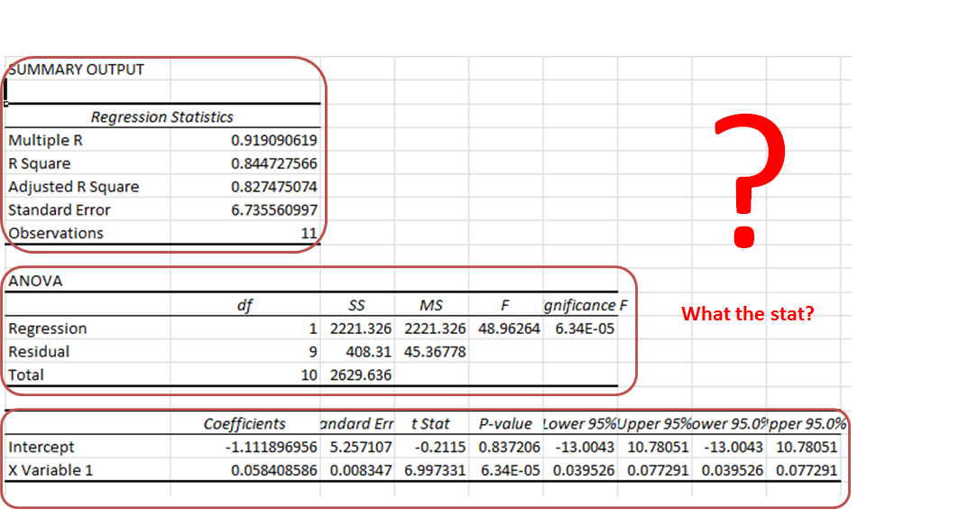
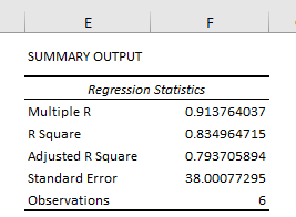
Summary Section:
As the name suggests, it is a summary of the data.

-
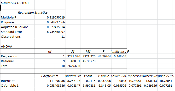
- Multiple R: It tells how fit the regression equation is to the data. It is also called the correlation coefficient.
In our case, it is 0.919090619 or 0.92 (roundup). This means that there is a 92% chance of an increase in sales if we increase our salesmen count.
-
- R Square: It tells the reliability of found regression. It tells us how many observations are part of our line of regression. In our case, it is 0.844727566 or 0.85. It means that our regression is fit by 85%.
- Adjusted R Square: Theadjusted square is just a more testified version of R square. Mainly useful in Multiple Regression Analysis.
- Standard Error: While R. Squire tells you how many data points fall near the regression line, the standard error tells you how far a data point can go from the regression line.
In our case, it is 6.74.
- Observation: This is simply the number of observations, which is 11 in our example.
Anova Section:
This section is hardly used in linear regression.
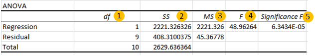
- df. It is a degree of freedom. It is used when calculating regression manually.
- SS. Sum of squares. It is just a sum of squares of variances. Used to find R squire values.
- MS. This means squared value.
- And 5. F and Significance of F. If the significance of F (p-value of the slope) is less than the F test than you can discard the null hypothesis and prove your hypothesis. In simple language, you can conclude that there is some effect of x on y when changed.
In our case, F is 48.96264 and Significance of F is 0.000063. It means our regression fits the data.
Regression Section:
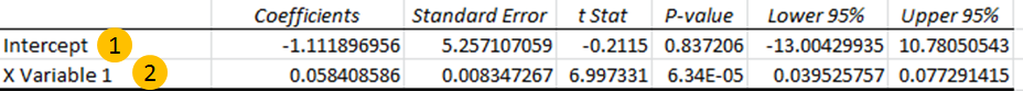
In this section, we have the two most important values for our regression equation.
- Intercept: We have an intercept here that tells where x-intercepts on Y. This is an important part of the regression equation. It is -1.11 in our case.
- X variable 1 (Slope). Also called the coefficient of x. It defines the tangent of the regression line.
REGRESSION CHART IN EXCEL
In excel, it is easy to plot a regression chart. Just follow these steps. To add Regression Chart in Excel 2016, 2013, and 2010 follow these simple steps.
Step 1. Have your known x’s in the first column and know y’s in the second.
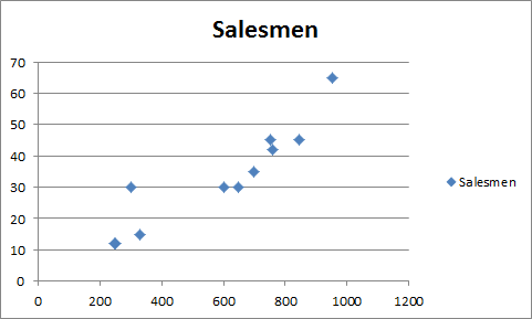
In our case, we know Known_ x’s are Soft Drinks Sold. And known_y’s are Salesmen.

Step 2. Select your known x’s and y’s range.

Step 3: Go to the Insert tab and click on the scatter chart.
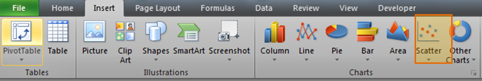
You will have a chart that looks like this.
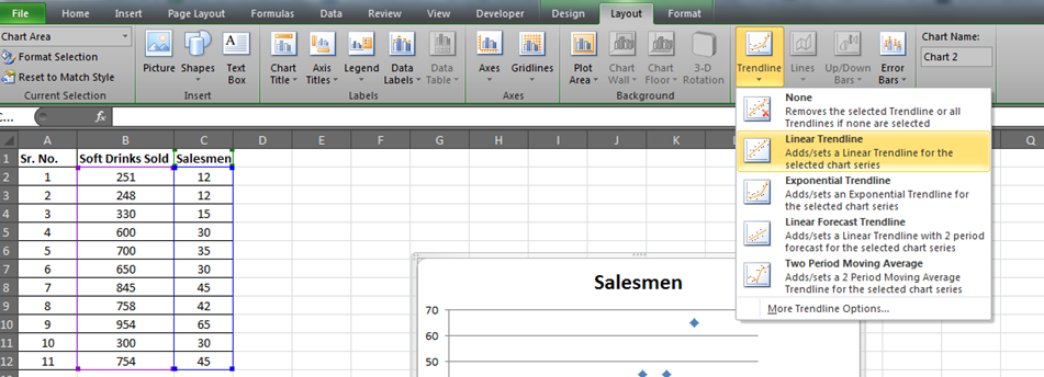
Step 4. Add the trend line: Goto layout and locate the trendline option in the analysis section.
Under the Trendline option, click on Linear Trendline.
You will have your graph looking like this.
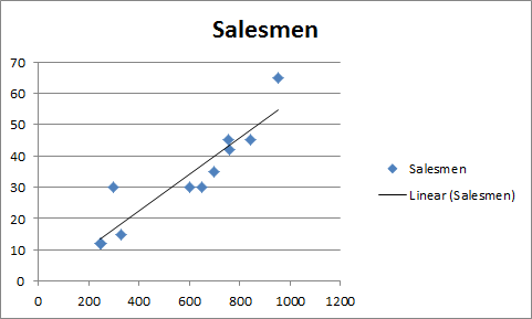
This is your regression graph.
Now if you add the data below and extend the selected data. You will see a change in your graph.
For our example, we added 2000 to the Soft Drink Sold and left the Salesmen blank. And when we extend the range of the graph, this is what we will have.
It will give the required number of salesmen for doing 2000 sales of soft drinks in graphical form. Which is slightly below 120 in the graph. And from our regression equation, we know it is 116.

In this article, I tried to cover everything under Excel Regression Analysis. I explained regression in excel 2016. Regression in excel 2010 and excel 2013 is same as in excel 2016.
For any further query on this topic, use the comments section. Ask a question, give an opinion or just mention my grammatical mistakes. Everything is welcome. Just don’t hesitate to use the comment section.
Related Data:
How to Use STDEV Function in Excel
How To Calculate MODE function in Excel
How To Calculate Mean function in Excel
How to Create Standard Deviation Graph
Descriptive Statistics in Microsoft Excel 2016
How to Use Excel NORMDIST Function
How to use the Pareto Chart and Analysis
Popular Articles:
50 Excel Shortcut to Increase Your Productivity
How to use the VLOOKUP Function in Excel
How to use the COUNTIF function in Excel 2016
How to use the SUMIF Function in Excel