
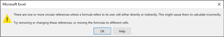
You’ve entered a formula, but it’s not working. Instead, you’ve got this message about a “circular reference.” Millions of people have the same problem and it happens because your formula is trying to calculate itself. Here’s what it looks like:
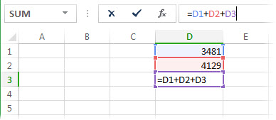
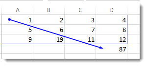
The formula =D1+D2+D3 breaks because it lives in cell D3, and it’s trying to calculate itself. To fix the problem, you can move the formula to another cell. Press Ctrl+X to cut the formula, select another cell, and press Ctrl+V to paste it.
Tips:
-
At times, you may want to use circular references because they cause your functions to iterate. If this is the case, jump down to Learn more about iterative calculation.
-
Also, see Overview of formulas in Excel to learn more about writing formulas.
Another common mistake is using a function that includes a reference to itself; for example, cell F3 contains =SUM(A3:F3). Here’s an example:

You can also try one of these techniques:
-
If you just entered a formula, start with that cell and check to see if you refer to the cell itself. For example, cell A3 might contain the formula =(A1+A2)/A3. Formulas like =A1+1 (in cell A1) also cause circular reference errors.
While you’re looking, check for indirect references. They happen when you put a formula in cell A1, and it uses another formula in B1 that in turn refers back to cell A1. If this confuses you, imagine what it does to Excel.
-
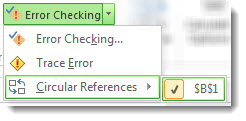
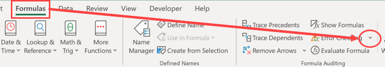
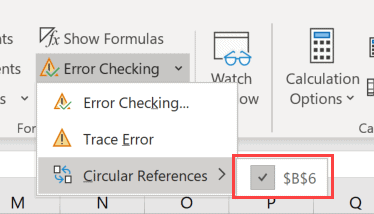
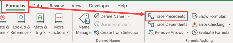
If you can’t find the error, click the Formulas tab, click the arrow next to Error Checking, point to Circular References, and then click the first cell listed in the submenu.

-
Review the formula in the cell. If you can’t determine whether the cell is the cause of the circular reference, click the next cell in the Circular References submenu.
-
Continue to review and correct the circular references in the workbook by repeating steps any or all of the steps 1 through 3 until the status bar no longer displays «Circular References.»
Tips
-
If you’re brand new to working with formulas, see Excel 2016 Essential Training at LinkedIn Learning.
-
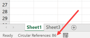
The status bar in the lower-left corner displays Circular References and the cell address of one circular reference.
If you have circular references in other worksheets, but not in the active worksheet, the status bar displays only “Circular References” with no cell addresses.
-
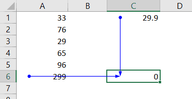
You can move between cells in a circular reference by double-clicking the tracer arrow. The arrow indicates the cell that affects the value of the currently selected cell. You show the tracer arrow by clicking Formulas, and then click either Trace Precedents or Trace Dependents.

Learn about the circular reference warning message
The first time Excel finds a circular reference, it displays a warning message. Click OK or close the message window.
When you close the message, Excel displays either a zero or the last calculated value in the cell. And now you’re probably saying, «Hang on, a last calculated value?» Yes. In some cases, a formula can run successfully before it tries to calculate itself. For example, a formula that uses the IF function may work until a user enters an argument (a piece of data the formula needs to run properly) that causes the formula to calculate itself. When that happens, Excel retains the value from the last successful calculation.
If you suspect you have a circular reference in a cell that isn’t showing a zero, try this:
-
Click the formula in the formula bar, and then press Enter.
Important In many cases, if you create additional formulas that contain circular references, Excel won’t display the warning message again. The following list shows some, but not all, the scenarios in which the warning message will appear:
-
You create the first instance of a circular reference in any open workbook
-
You remove all circular references in all open workbooks, and then create a new circular reference
-
You close all workbooks, create a new workbook, and then enter a formula that contains a circular reference
-
You open a workbook that contains a circular reference
-
While no other workbooks are open, you open a workbook and then create a circular reference
Learn about iterative calculation
At times, you may want to use circular references because they cause your functions to iterate—repeat until a specific numeric condition is met. This can slow your computer down, so iterative calculations are usually turned off in Excel.
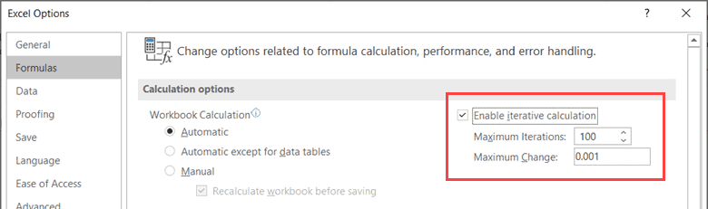
Unless you’re familiar with iterative calculations, you probably won’t want to keep any circular references intact. If you do, you can enable iterative calculations, but you need to determine how many times the formula should recalculate. When you turn on iterative calculations without changing the values for maximum iterations or maximum change, Excel stops calculating after 100 iterations, or after all values in the circular reference change by less than 0.001 between iterations, whichever comes first. However, you can control the maximum number of iterations and the amount of acceptable change.
-
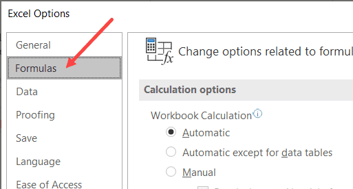
Click File > Options > Formulas. If you’re using Excel for Mac, click the Excel menu, and then click Preferences > Calculation.
-
In the Calculation options section, select the Enable iterative calculation check box. On the Mac, click Use iterative calculation.
-
To set the maximum number of times that Excel will recalculate, type the number of iterations in the Maximum Iterations box. The higher the number of iterations, the more time that Excel needs to calculate a worksheet.
-
In the Maximum Change box, type the smallest value required for iteration to continue. This is the smallest change in any calculated value. The smaller the number, the more precise the result and the more time that Excel needs to calculate a worksheet.
An iterative calculation can have three outcomes:
-
The solution converges, which means a stable end result is reached. This is the desirable condition.
-
The solution diverges, which means that from iteration to iteration, the difference between the current and the previous result increases.
-
The solution switches between two values. For example, after the first iteration the result is 1, after the next iteration the result is 10, after the next iteration the result is 1, and so on.
Top of Page
Need more help?
You can always ask an expert in the Excel Tech Community or get support in the Answers community.

Tip: If you’re a small business owner looking for more information on how to get Microsoft 365 set up, visit Small business help & learning.
See also
Excel 2016 Essential Training
Overview of formulas in Excel
How to avoid broken formulas
Find and correct errors in formulas
Excel keyboard shortcuts and function keys
Excel functions (alphabetical)
Excel functions (by category)
Содержание
- Выявление циклических связей
- Способ 1: кнопка на ленте
- Способ 2: стрелка трассировки
- Вопросы и ответы
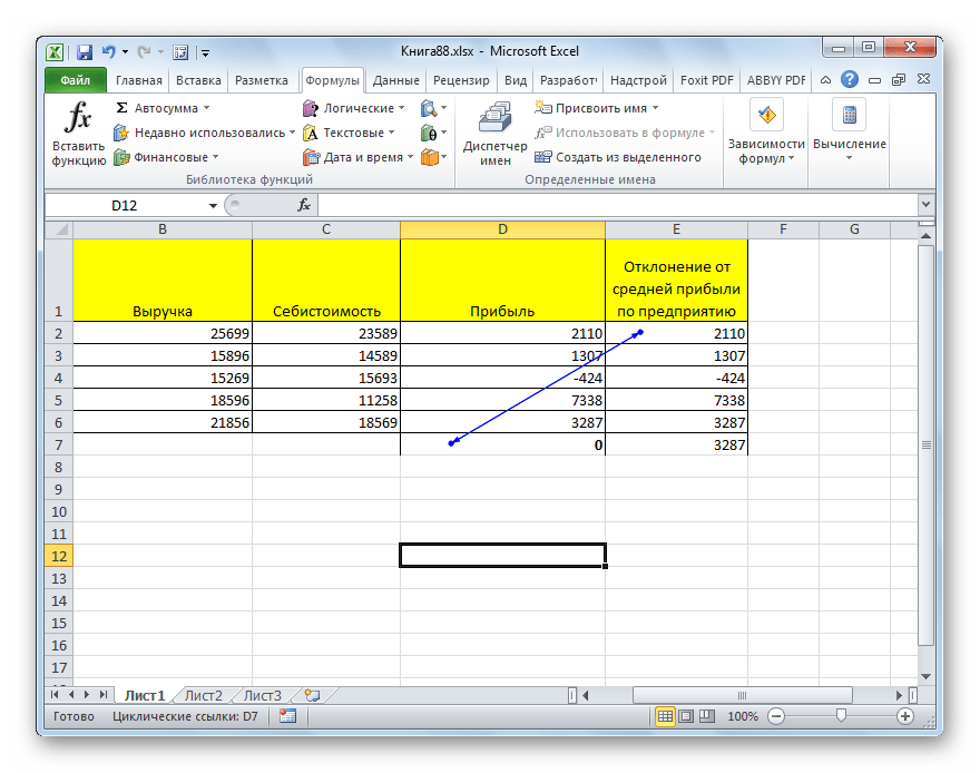
Циклические ссылки представляют собой формулу, в которой одна ячейка через последовательность связей с другими ячейками, в конечном итоге ссылается сама на себя. В некоторых случаях пользователи осознано применяют подобный инструмент для вычислений. Например, такой подход может помочь при моделировании. Но, в большинстве случаев, данная ситуация – это просто ошибка в формуле, которую юзер допустил по невнимательности или по другим причинами. В связи с этим, чтобы удалить ошибку, следует сразу найти саму циклическую ссылку. Посмотрим, как это делается.
Выявление циклических связей
Если в книге присутствует циклическая ссылка, то уже при запуске файла программа в диалоговом окне предупредит об этом факте. Так что с определением самого наличия такой формулы проблем не возникнет. Как же найти проблемную область на листе?
Способ 1: кнопка на ленте
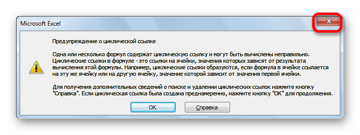
- Чтобы узнать, в каком именно диапазоне находится такая формула, прежде всего, жмем на кнопку в виде белого крестика в красном квадрате в диалоговом окне предупреждения, тем самым закрывая его.
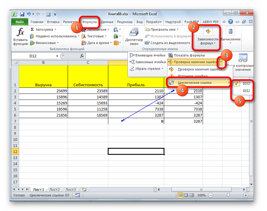
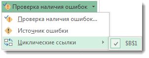
- Переходим во вкладку «Формулы». На ленте в блоке инструментов «Зависимости формул» имеется кнопка «Проверка наличия ошибок». Кликаем на пиктограмму в виде перевернутого треугольника рядом с этой кнопкой. В появившемся меню выбираем пункт «Циклические ссылки». После перехода по этой надписи в виде меню показываются все координаты ссылок циклического характера в данной книге. При клике на координаты конкретной ячейки, она становится активной на листе.
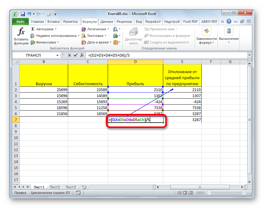
- Путем изучения результата устанавливаем зависимость и устраняем причину цикличности, если она вызвана ошибкой.
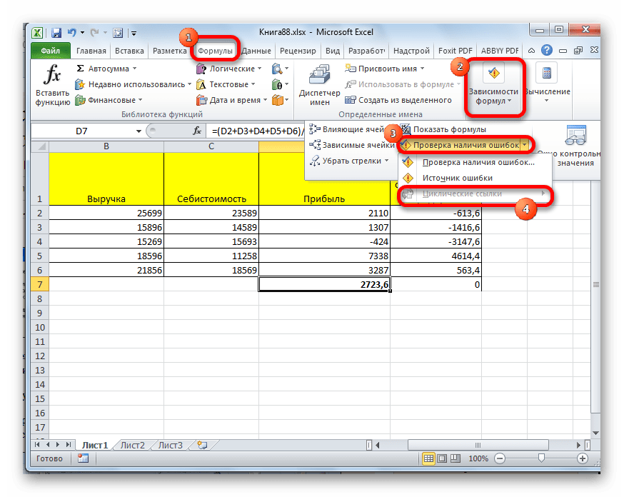
- После выполнения необходимых действий снова переходим по кнопке проверки ошибок циклических ссылок. На этот раз соответствующий пункт меню должен быть вообще не активен.
Способ 2: стрелка трассировки
Существует и другой способ определения подобных нежелательных зависимостей.
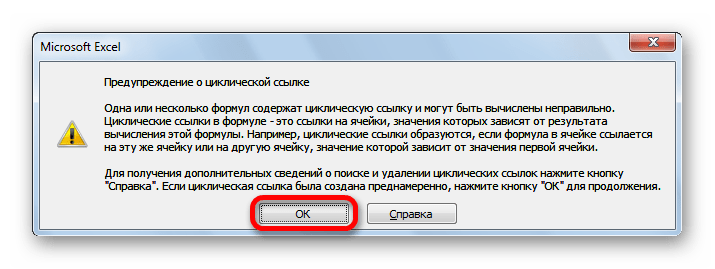
- В диалоговом окне, сообщающем о наличии циклических ссылок, жмем на кнопку «OK».
- Появляется стрелка трассировки, которая указывает зависимости данных в одной ячейки от другой.
Нужно отметить, что второй способ более визуально нагляден, но в то же время не всегда даёт четкую картину цикличности, в отличие от первого варианта, особенно в сложных формулах.
Как видим, отыскать циклическую ссылку в Эксель довольно просто, особенно если знать алгоритм поиска. Можно воспользоваться одним из двух способов нахождения подобных зависимостей. Несколько сложнее определить, нужна ли данная формула в действительно или это просто ошибка, а также исправить ошибочную ссылку.
Еще статьи по данной теме:
Помогла ли Вам статья?
![]()
Download Article
The complete guide to fixing circular reference errors
![]()
Download Article
- What is a circular reference?
- Find and Fix Circular References
- Enable Iterative Calculations
- Tips
|
|
|
Are you seeing an error about a «circular reference» when you try to edit an Excel worksheet? A circular reference is when a formula tries to calculate itself while iterative calculation is disabled. Fortunately, it’s easy to find and fix the circular references in your data. You can use the Error Checking feature to locate the cells with formulas that contain circular references and use a formula to fix them. Alternatively, you can enable iterative calculations to allow them. This wikiHow shows you how to find and fix or allow a circular reference in Microsoft Excel.
Things You Should Know
- A circular reference is when a formula tries to calculate itself.
- Go to Formulas > Error Checking > Circular References to see a list of circular references.
- Enable “iterative calculations” in the options menu to allow circular references to run.
-
1
A circular reference is when a formula refers to the cell it’s being written in. This means the Excel formula you made is trying to incorporate itself into the formula, creating a loop. Cells with a circular reference will show a zero or the last calculated value. There are two common ways a circular reference occurs:[1]
- Direct reference: The formula refers to the cell it’s being written in.
- Indirect reference: The formula refers to another cell that refers to the cell the formula is being written in.
-
2
Check out this example of a direct circular reference. Let’s say you’re trying to add the values of cells A1, A2, and A3. You write the summation formula “=A1+A2+A3+A4” in cell A4. This causes a circular reference, since the summation formula includes the cell it’s being written in, A4.
Advertisement
-
3
Check out this example of an indirect circular reference. You add the values in D2 and E2 with a formula in D3: “=D2+E2”. Then you create another formula in E2: “=D2+D3”. Now, the formula in D3 references the formula in E2, which includes D3, creating an indirect circular reference.


Advertisement
-
1
Click Formulas. This is a tab at the top of Excel. Fixing a formula in Excel can be tricky, but luckily the software has built-in error checking!
-
2
Click the Error Checking down arrow. This will open a drop down menu with error checking options.
-
3
Hover your cursor over Circular References. This will show you the next circular reference in the current worksheet.
-
4
Click the cell in the Circular References list. This will take you to the cell with the circular reference. These can sometimes occur when you copy and paste formulas, since the cell references can shift.
-
5
Review the cell’s formula. Check whether the cell includes a reference to itself. If the formula is complicated or your worksheet has a complex workflow of formulas, use Trace Precedents and Trace Dependents to see what cells the formula refers to and affects:
- Select the cell with the circular reference error.
- Click the Formulas tab.
- Click Trace Precedents to see what cells the formula uses.
- Click Trace Dependents to see what cells have formulas referencing the cell you selected.


Advertisement
-
1
Open the calculation options. This method turns on Iterative Calculations in the options menu. This allows formulas with circular references to recalculate a specified number of times. This can slow down the Excel file, especially for complex formulas. To open the calculation options:
- Windows:
- Click the File tab.
- Click Options in the left sidebar.
- Click Formulas in the Options window’s sidebar.
- Mac:
- Click the Excel menu bar item.
- Click Preferences in the drop down menu.
- Select Calculation.
- Windows:
-
2
Click the box next to “Enable iterative calculation” (Windows). This is called “Use iterative calculation” on Mac.
-
3
Change the Maximum Iterations and Maximum Change values (optional). Excel will recalculate the circular reference formula either when it has iterated the maximum amount of times, or when the calculated values in the formula differ by less than the maximum change.
- Increasing the Maximum Iterations or decreasing the Maximum Change will increase the calculation time.


Advertisement
Ask a Question
200 characters left
Include your email address to get a message when this question is answered.
Submit
Advertisement
Thanks for submitting a tip for review!
Advertisement
About This Article
Thanks to all authors for creating a page that has been read 457 times.
Is this article up to date?
While working with Excel formulas, you may sometime see the following warning prompt.
This prompt tells you that there is a circular reference in your worksheet and this can lead or an incorrect calculation by the formulas. It also asks you to address this circular reference issue and sort it.
In this tutorial, I will cover all that you need to know about circular reference, and well as how to find and remove circular references in Excel.
So let’s get started!
What is Circular Reference in Excel?
In simple words, a circular reference happens when you end up having a formula in a cell – which in itself uses the cell (in which it’s been entered) for the calculation.
Let me try and explain this by a simple example.
Suppose you have the dataset in cell A1:A5 and you use the below formula in cell A6:
=SUM(A1:A6)
This will give you a circular reference warning.
This is because you want to sum the values in cell A1:A6, and the result should be in cell A6.
This creates a loop as Excel just keeps on adding the new value in cell A6, which keeps on changing (hence, a circular reference loop).
How to Find Circular References in Excel?
While the circular reference warning prompt is kind enough to tell you that it exists in your worksheet, it doesn’t tell you where it’s happening and what cell references are causing it.
So if you’re trying to find and handle circular references in the worksheet, you need to know a way to somehow find these.
Below are the steps to find a circular reference in Excel:
- Activate the worksheet that has the circular reference
- Click the Formulas tab
- In the Formula Editing group, click on the Error Checking drop-down icon (little downward pointing arrow at the right)

- Hover the cursor over the Circular References option. It will show you the cell that has a circular reference in the worksheet

- Click on the cell address (that is displayed) and it will take you to that cell in the worksheet.
Once you have addressed the issue, you can again follow the same steps above and it will show more cell references that have the circular reference. If there is none, you will not see any cell reference,
Another quick and easy way to find the circular reference is by looking at the Status bar. On the left part of it, it will show you the text Circular Reference along with the cell address.
There are a few things you need to know when working with circular references:
- In case the iterative calculation is enabled (covered later in this tutorial), the status bar will not show the circular reference cell address
- In case the circular reference is not in the active sheet (but in other sheets in the same workbook), it will only show Circular reference and not the cell address
- In case you get a circular reference warning prompt once and you dismiss it, it will not show the prompt again the next time.
- If you open a workbook that has the circular reference, it will show you the prompt as soon as the workbook opens.
How to Remove a Circular Reference in Excel?
Once you have identified that there are circular references in your sheet, it’s time to remove these (unless you want them to be there for a reason).
Unfortunately, it’s not as simple as hitting the delete key. Since these are dependent on formulas and every formula is different, you need to analyze this on a case-by-case basis.
In case it’s just a matter of having the cell reference causing the issue by mistake, you can simply correct by adjusting the reference.
But sometimes, it’s not that simple.
Circular reference can also be caused based on multiple cells that feed into each other at many levels.
Let me show you an example.
Below there is a circular reference in cell C6, but it’s not just a simple case of self-reference. It’s multi-level where the cells it uses in the calculations also reference each other.
- The formulas in cell A6 is =SUM(A1:A5)+C6
- The formula is cell C1 is =A6*0.1
- The formula in cell C6 is =A6+C1
In the above example, the result in cell C6 is dependent on the values in cell A6 and C1, which in turn are dependent on cell C6 (thus causing the circular reference error)
And again, I have chosen a really simple example just for demo purposes. In reality, these could be quite difficult to figure out and maybe far off in the same worksheet or even scattered across multiple worksheets.
In such a case, there is one way to identify the cells that are causing circular reference and then treat these.
It’s by using the Trace Precedents option.
Below are the steps to use trace precedents to find cells that are feeding to the cell that has the circular reference:
- Select the cell that has the circular reference
- Click the Formulas tab
- Click on Trace Precedents

The above steps would show you blue arrows which will tell you what cells are feeding into the formula in the selected cell. This way, you can inspect the formulas and the cells and get rid of the circular reference.
In case you’re working with complex financial models, it may be possible that these precedents also go multiple levels deep.
This works well if you have all the formulas referring to cells in the same worksheet. If it’s in multiple worksheets, this method is not effective.
How to Enable/Disable Iterative Calculations in Excel
When you have a circular reference in a cell, first you get the warning prompt as shown below, and if you close this dialog box, it will give you 0 as the result in the cell.
This is because when there is a circular reference, it’s an endless loop and Excel doesn’t want to caught up in it. So it returns a 0.
But in some cases, you may actually want the circular reference to be active and do a couple of iterations. In such a case, instead of an infinite loop, and you can decide how many times the loop should be run.
This is called iterative calculation in Excel.
Below are the steps to enable and configure iterative calculations in Excel:
- Click the File tab
- Click on Options. This will open the Excel Options dialog box
- Select Formula in the left pane

- In the Calculation options section, check the box ‘Enable iterative calculation’. Here you can specify the maximum iterations and maximum change value

That’s it! The above steps would enable iterative calculation in Excel.
Let me also quickly explain the two options in the iterative calculation:
- Maximum iterations: This is the maximum number of times you want Excel to calculate before giving you the final result. So if you specify this as 100, Excel will run the loop 100 times before giving you the final result.
- Maximum Change: This is the maximum change, which if not achieved between iterations, the calculation would be stopped. By default, the value is .001. The lower this value, the more accurate would be the result.
Remember that the more number of times the iterations run, the more time and resources it takes for Excel to do it. In case you keep the maximum iterations high, it may lead to your Excel slowing down or crashing.
Note: When iterative calculations are enabled, Excel will not show you the circular reference warning prompt and will also now show it in the status bar.
Deliberately Using Circular References
In most cases, the presence of circular reference in your worksheet would be an error. And this is why Excel shows you a prompt which says – “Try removing or changing these references or moving the formulas to different cells.”
But there might be some specific cases where you need a circular reference so that you can get the desired result.
One such specific case I have already written about it getting the time stamp in a cell in a cell in Excel.
For example, suppose you want to create a formula so that every an entry is made in a cell in Column A, the timestamp appear in Column B (as shown below):
While you can insert easily insert a timestamp using the below formula:
=IF(A2<>"",IF(B2<>"",B2,NOW()),"")
The issue with the above formula is that it would update all the timestamps as soon as any change is made in the worksheet or if the worksheet is reopened (as the NOW formula is volatile)
To get around this issue, you can use a circular reference method. Use the same formula, but enable iterative calculation.
There are some other cases as well where having the ability to use circular reference is desired (you can find one example here).
Note: While there may be some cases where you can use circular reference, I find it best to avoid using it. Circular references can also take a toll on the performance of your workbook and can make it slow. In rare cases where you need it, I always prefer using VBA codes to get the work done.
I hope you found this tutorial useful!
Other Excel tutorials you may find useful:
- #REF! Error in Excel; How to Fix the Reference Error!
- Excel VBA Error Handling
- Use IFERROR with VLOOKUP to Get Rid of #N/A Errors
- How to Reference Another Sheet or Workbook in Excel (with Examples)
- Absolute, Relative, and Mixed Cell References in Excel
Содержание
- Как найти круговую ссылку в Excel (быстро и легко)
- Что такое круговая ссылка в Excel?
- Как найти круговые ссылки в Excel?
- Как удалить круговую ссылку в Excel?
- Как включить / отключить итерационные вычисления в Excel
- Умышленное использование круговых ссылок
- Удаление или разрешение циклической ссылки
- Предупреждение о циклической ссылке
- Итеративные вычисления
- Дополнительные сведения
Как найти круговую ссылку в Excel (быстро и легко)

При работе с формулами Excel вы можете иногда увидеть следующее предупреждение.
Это приглашение сообщает вам, что на вашем листе есть циклическая ссылка, и это может привести к неправильному расчету по формулам. Он также просит вас решить эту проблему с циклическими ссылками и отсортировать ее.
В этом уроке я расскажу все, что вам нужно знать о круговой ссылке, а также как найти и удалить циклические ссылки в Excel.
Что такое круговая ссылка в Excel?
Проще говоря, циклическая ссылка возникает, когда вы в конечном итоге получаете формулу в ячейке, которая сама по себе использует ячейку (в которую она была введена) для вычисления.
Позвольте мне попытаться объяснить это на простом примере.
Предположим, у вас есть набор данных в ячейке A1: A5, и вы используете приведенную ниже формулу в ячейке A6:
Это даст вам предупреждение о круговой ссылке.
Это потому, что вы хотите просуммировать значения в ячейке A1: A6, и результат должен быть в ячейке A6.
Это создает цикл, поскольку Excel просто продолжает добавлять новое значение в ячейку A6, которое продолжает меняться (следовательно, цикл циклической ссылки).
Как найти круговые ссылки в Excel?
Хотя предупреждение о циклической ссылке достаточно любезно, чтобы сообщить вам, что оно существует на вашем листе, оно не сообщает вам, где это происходит и какие ссылки на ячейки вызывают это.
Поэтому, если вы пытаетесь найти и обработать циклические ссылки на листе, вам нужно знать способ как-то их найти.
Ниже приведены шаги, чтобы найти циклическую ссылку в Excel:
- Активируйте рабочий лист с круговой ссылкой
- Перейдите на вкладку «Формулы».
- В группе «Редактирование формул» щелкните раскрывающийся значок «Проверка ошибок» (маленькая стрелка, направленная вниз, справа).
- Наведите курсор на опцию Циркулярные ссылки. Он покажет вам ячейку с круговой ссылкой на листе.
- Щелкните адрес ячейки (который отображается), и вы перейдете к этой ячейке на листе.


Решив проблему, вы можете снова выполнить те же действия, описанные выше, и он покажет больше ссылок на ячейки, которые имеют циклическую ссылку. Если его нет, вы не увидите ссылку на ячейку,
Еще один быстрый и простой способ найти круговую ссылку — это посмотреть на строку состояния. В левой его части будет отображаться текст Циркулярная ссылка вместе с адресом ячейки.

При работе с круговыми ссылками необходимо знать несколько вещей:
- Если включено итеративное вычисление (описанное далее в этом руководстве), в строке состояния не будет отображаться адрес ячейки с круговой ссылкой.
- В случае, если круговая ссылка отсутствует на активном листе (а на других листах в той же книге), будет отображаться только круговая ссылка, а не адрес ячейки.
- Если вы получили предупреждение о циклической ссылке один раз и отклонили его, в следующий раз оно больше не будет отображаться.
- Если вы откроете книгу с циклической ссылкой, она отобразит подсказку, как только откроется книга.
Как удалить круговую ссылку в Excel?
Как только вы определили, что на вашем листе есть циклические ссылки, пора их удалить (если вы не хотите, чтобы они были там по какой-либо причине).
К сожалению, это не так просто, как нажать клавишу удаления. Поскольку они зависят от формул, а каждая формула отличается, вам необходимо анализировать это в каждом конкретном случае.
Если проблема вызвана ошибкой ссылки на ячейку, вы можете просто исправить ее, изменив ссылку.
Но иногда все не так просто.
Круговая ссылка также может быть вызвана на основе нескольких ячеек, которые взаимодействуют друг с другом на многих уровнях.
Позвольте мне показать вам пример.
Ниже в ячейке C6 есть циклическая ссылка, но это не просто случай ссылки на самого себя. Он многоуровневый, где ячейки, которые он использует в вычислениях, также ссылаются друг на друга.

- Формула в ячейке A6: = СУММ (A1: A5) + C6.
- Формула: ячейка C1 = A6 * 0,1
- Формула в ячейке C6: = A6 + C1.
В приведенном выше примере результат в ячейке C6 зависит от значений в ячейках A6 и C1, которые, в свою очередь, зависят от ячейки C6 (что вызывает ошибку циклической ссылки)
И снова я выбрал очень простой пример только для демонстрационных целей. На самом деле, это может быть довольно сложно понять, и, возможно, они находятся далеко на одном листе или даже разбросаны по нескольким листам.
В таком случае есть один способ идентифицировать ячейки, которые вызывают циклическую ссылку, и затем обработать их.
Это можно сделать с помощью параметра «Отслеживать прецеденты».
Ниже приведены шаги по использованию прецедентов трассировки для поиска ячеек, которые передаются в ячейку с циклической ссылкой:
- Выберите ячейку с круговой ссылкой
- Перейдите на вкладку «Формулы».
- Нажмите на прецеденты трассировки

Приведенные выше шаги покажут вам синие стрелки, которые укажут, какие ячейки вводятся в формулу в выбранной ячейке. Таким образом, вы можете проверить формулы и ячейки и избавиться от циклической ссылки.
Если вы работаете со сложными финансовыми моделями, вполне возможно, что эти прецеденты также имеют несколько уровней глубины.
Это хорошо работает, если у вас есть все формулы, относящиеся к ячейкам на одном листе. Если это на нескольких листах, этот метод неэффективен.
Как включить / отключить итерационные вычисления в Excel
Когда у вас есть круговая ссылка в ячейке, сначала вы получаете предупреждение, как показано ниже, и если вы закроете это диалоговое окно, в качестве результата в ячейке вы получите 0.
Это связано с тем, что циклическая ссылка представляет собой бесконечный цикл, и Excel не хочет зацикливаться на нем. Таким образом, он возвращает 0.
Но в некоторых случаях вам может потребоваться активировать циклическую ссылку и выполнить пару итераций. В таком случае вместо бесконечного цикла вы можете решить, сколько раз цикл должен быть запущен.
Это называется итерационный расчет в Excel.
Ниже приведены шаги для включения и настройки итерационных вычислений в Excel:
- Перейдите на вкладку Файл.
- Щелкните Параметры. Откроется диалоговое окно «Параметры Excel».
- Выберите формулу на левой панели
- В разделе «Параметры расчета» установите флажок «Включить итерационный расчет». Здесь вы можете указать максимальное количество итераций и максимальное значение изменения


Вот и все! Вышеупомянутые шаги позволят выполнить итеративный расчет в Excel.
Позвольте мне также быстро объяснить два варианта итеративного расчета:
- Максимальное количество итераций: Это максимальное количество раз, которое вы хотите, чтобы Excel вычислил, прежде чем выдает окончательный результат. Поэтому, если вы укажете это как 100, Excel выполнит цикл 100 раз, прежде чем выдаст вам окончательный результат.
- Максимальное изменение: Это максимальное изменение, которое, если не достигнуто между итерациями, вычисление будет остановлено. По умолчанию это значение 0,001. Чем ниже это значение, тем точнее будет результат.
Помните, что чем больше раз выполняются итерации, тем больше времени и ресурсов у Excel уходит на это. Если вы сохраните максимальное количество итераций на высоком уровне, это может привести к замедлению работы Excel или сбою.
Примечание. Когда включены итеративные вычисления, Excel не будет отображать предупреждение о циклической ссылке, а также теперь будет отображать его в строке состояния.
Умышленное использование круговых ссылок
В большинстве случаев наличие круговой ссылки на вашем листе будет ошибкой. Вот почему Excel показывает подсказку: «Попробуйте удалить или изменить эти ссылки или переместить формулы в другие ячейки».
Но могут быть некоторые конкретные случаи, когда вам понадобится круговая ссылка, чтобы вы могли получить желаемый результат.
Один такой конкретный случай, о котором я уже писал, получение отметки времени в ячейке в ячейке в Excel.
Например, предположим, что вы хотите создать формулу, чтобы каждая запись производилась в ячейке в столбце A, а метка времени отображалась в столбце B (как показано ниже):

Хотя вы можете легко вставить метку времени, используя следующую формулу:
Проблема с приведенной выше формулой заключается в том, что она обновит все временные метки, как только на листе будет внесено какое-либо изменение или если рабочий лист будет повторно открыт (поскольку формула СЕЙЧАС является изменчивой)
Чтобы обойти эту проблему, вы можете использовать метод круговой ссылки. Используйте ту же формулу, но разрешите итеративный расчет.
Есть и другие случаи, когда желательна возможность использовать циклическую ссылку (вы можете найти здесь один пример).
Примечание. Хотя в некоторых случаях можно использовать круговую ссылку, я считаю, что лучше избегать ее использования. Циркулярные ссылки также могут сказаться на производительности вашей книги и замедлить ее. В редких случаях, когда вам это нужно, я всегда предпочитаю использовать коды VBA для выполнения работы.
Надеюсь, вы нашли этот урок полезным!
Другие учебники по Excel могут оказаться полезными:
- # ССЫЛКА! Ошибка в Excel; Как исправить ошибку ссылки!
- Обработка ошибок Excel VBA
- Используйте ЕСЛИОШИБКА с функцией ВПР, чтобы избавиться от # ошибок Н / Д
- Как сослаться на другой лист или книгу в Excel (с примерами)
- Абсолютные, относительные и смешанные ссылки на ячейки в Excel
Источник
Удаление или разрешение циклической ссылки
Вы ввели формулу, но она не работает. Вместо этого вы получили сообщение о «циклической ссылке». Миллионы людей имеют ту же проблему, и это происходит потому, что ваша формула пытается вычислить себя. Вот как это выглядит:

Формула =D1+D2+D3 не работает, поскольку она расположена в ячейке D3 и ссылается на саму себя. Чтобы устранить проблему, можно переместить формулу в другую ячейку. Нажмите клавиши CTRL+X , чтобы вырезать формулу, выделите другую ячейку и нажмите клавиши CTRL+V , чтобы вставить ее.
Иногда может потребоваться использовать циклические ссылки, так как они вызывают итерацию функций. В этом случае перейдите к статье Дополнительные сведения о итеративном вычислении.
Другая распространенная ошибка связана с использованием функций, которые включают ссылки на самих себя, например ячейка F3 может содержать формулу =СУММ(A3:F3). Пример:

Вы также можете попробовать один из описанных ниже способов.
Если вы только что ввели формулу, начните с этой ячейки и проверьте, ссылаетесь ли вы на саму ячейку. Например, ячейка A3 может содержать формулу =(A1+A2)/A3. Такие формулы, как =A1+1 (в ячейке A1), также вызывают ошибки циклической ссылки.
Проверьте наличие непрямых ссылок. Они возникают, когда формула, расположенная в ячейке А1, использует другую формулу в ячейке B1, которая снова ссылается на ячейку А1. Если это сбивает с толку вас, представьте, что происходит с Excel.
Если найти ошибку не удается, на вкладке Формулы щелкните стрелку рядом с кнопкой Проверка ошибок, выберите пункт Циклические ссылки и щелкните первую ячейку в подменю.
Проверьте формулу в ячейке. Если вам не удается определить, является ли эта ячейка причиной циклической ссылки, выберите в подменю Циклические ссылки следующую ячейку.
Продолжайте находить и исправлять циклические ссылки в книге, повторяя действия 1–3, пока из строки состояния не исчезнет сообщение «Циклические ссылки».
В строке состояния в левом нижнем углу отображается сообщение Циклические ссылки и адрес ячейки с одной из них.
При наличии циклических ссылок на других листах, кроме активного, в строке состояния выводится сообщение «Циклические ссылки» без адресов ячеек.
Вы можете перемещаться между ячейками в циклической ссылке, дважды щелкнув стрелку трассировки. Стрелка указывает ячейку, которая влияет на значение выбранной ячейки. Стрелка трассировки отображается, щелкнув Формулы, а затем — Прецеденты трассировки или Трассировка Зависимости.
Предупреждение о циклической ссылке
Когда Excel впервые находит циклическую ссылку, появляется предупреждающее сообщение. Нажмите кнопку ОК или закройте окно сообщения.
При закрытии сообщения Excel отображает нулевое или последнее вычисляемое значение в ячейке. И теперь вы, вероятно, говорите: «Повесьте, последнее вычисляемое значение?» Да. В некоторых случаях формула может успешно выполниться до того, как она попытается вычислить себя. Например, формула, использующая функцию IF , может работать до тех пор, пока пользователь не введет аргумент (фрагмент данных, необходимый для правильного выполнения формулы), который приведет к вычислению самой формулы. В этом случае Excel сохраняет значение из последнего успешного вычисления.
Если есть подозрение, что циклическая ссылка содержится в ячейке, которая не возвращает значение 0, попробуйте такое решение:
Щелкните формулу в строке формулы и нажмите клавишу ВВОД.
Важно Во многих случаях при создании дополнительных формул с циклическими ссылками предупреждающее сообщение в приложении Excel больше не отображается. Ниже перечислены некоторые, но не все, ситуации, в которых предупреждение появится.
Пользователь создает первый экземпляр циклической ссылки в любой открытой книге.
Пользователь удаляет все циклические ссылки во всех открытых книгах, после чего создает новую циклическую ссылку.
Пользователь закрывает все книги, создает новую и вводит в нее формулу с циклической ссылкой.
Пользователь открывает книгу, содержащую циклическую ссылку.
При отсутствии других открытых книг пользователь открывает книгу и создает в ней циклическую ссылку.
Итеративные вычисления
Иногда может потребоваться использовать циклические ссылки, так как они вызывают итерацию функций— повторять до тех пор, пока не будет выполнено определенное числовое условие. Это может замедлить работу компьютера, поэтому итеративные вычисления обычно отключаются в Excel.
Если вы не знакомы с итеративными вычислениями, вероятно, вы не захотите оставлять активных циклических ссылок. Если же они вам нужны, необходимо решить, сколько раз может повторяться вычисление формулы. Если включить итеративные вычисления, не изменив предельное число итераций и относительную погрешность, приложение Excel прекратит вычисление после 100 итераций либо после того, как изменение всех значений в циклической ссылке с каждой итерацией составит меньше 0,001 (в зависимости от того, какое из этих условий будет выполнено раньше). Тем не менее, вы можете сами задать предельное число итераций и относительную погрешность.
Щелкните Файл > Параметры > Формулы. Если вы работаете в Excel для Mac, откройте меню Excel и выберите Настройки > Вычисление.
В разделе Параметры вычислений установите флажок Включить итеративные вычисления. На компьютере Mac щелкните Использовать итеративное вычисление.
В поле Предельное число итераций введите количество итераций для выполнения при обработке формул. Чем больше предельное число итераций, тем больше времени потребуется для пересчета листа.
В поле Относительная погрешность введите наименьшее значение, до достижения которого следует продолжать итерации. Это наименьшее приращение в любом вычисляемом значении. Чем меньше число, тем точнее результат и тем больше времени потребуется Excel для вычислений.
Итеративное вычисление может иметь три исход:
Решение сходится, что означает получение надежного конечного результата. Это самый желательный исход.
Решение расходится, т. е. при каждой последующей итерации разность между текущим и предыдущим результатами увеличивается.
Решение переключается между двумя значениями. Например, после первой итерации результат равен 1, после следующей итерации — 10, после следующей итерации — 1 и т. д.
Дополнительные сведения
Вы всегда можете задать вопрос специалисту Excel Tech Community или попросить помощи в сообществе Answers community.

Совет: Если вы владелец малого бизнеса и хотите получить дополнительные сведения о настройке Microsoft 365, посетите раздел Справка и обучение для малого бизнеса.
Источник
Содержание
- Что такое круговая ссылка в Excel?
- Как найти круговые ссылки в Excel?
- Как удалить круговую ссылку в Excel?
- Как включить / отключить итерационные вычисления в Excel
- Умышленное использование круговых ссылок
При работе с формулами Excel вы можете иногда увидеть следующее предупреждение.
Это приглашение сообщает вам, что на вашем листе есть циклическая ссылка, и это может привести к неправильному расчету по формулам. Он также просит вас решить эту проблему с циклическими ссылками и отсортировать ее.
В этом уроке я расскажу все, что вам нужно знать о круговой ссылке, а также как найти и удалить циклические ссылки в Excel.
Итак, приступим!
Проще говоря, циклическая ссылка возникает, когда вы в конечном итоге получаете формулу в ячейке, которая сама по себе использует ячейку (в которую она была введена) для вычисления.
Позвольте мне попытаться объяснить это на простом примере.
Предположим, у вас есть набор данных в ячейке A1: A5, и вы используете приведенную ниже формулу в ячейке A6:
= СУММ (A1: A6)
Это даст вам предупреждение о круговой ссылке.
Это потому, что вы хотите просуммировать значения в ячейке A1: A6, и результат должен быть в ячейке A6.
Это создает цикл, поскольку Excel просто продолжает добавлять новое значение в ячейку A6, которое продолжает меняться (следовательно, цикл циклической ссылки).
Как найти круговые ссылки в Excel?
Хотя предупреждение о циклической ссылке достаточно любезно, чтобы сообщить вам, что оно существует на вашем листе, оно не сообщает вам, где это происходит и какие ссылки на ячейки вызывают это.
Поэтому, если вы пытаетесь найти и обработать циклические ссылки на листе, вам нужно знать способ как-то их найти.
Ниже приведены шаги, чтобы найти циклическую ссылку в Excel:
- Активируйте рабочий лист с круговой ссылкой
- Перейдите на вкладку «Формулы».
- В группе «Редактирование формул» щелкните раскрывающийся значок «Проверка ошибок» (маленькая стрелка, направленная вниз, справа).
- Наведите курсор на опцию Циркулярные ссылки. Он покажет вам ячейку с круговой ссылкой на листе.
- Щелкните адрес ячейки (который отображается), и вы перейдете к этой ячейке на листе.
Решив проблему, вы можете снова выполнить те же действия, описанные выше, и он покажет больше ссылок на ячейки, которые имеют циклическую ссылку. Если его нет, вы не увидите ссылку на ячейку,
Еще один быстрый и простой способ найти круговую ссылку — это посмотреть на строку состояния. В левой его части будет отображаться текст Циркулярная ссылка вместе с адресом ячейки.
При работе с круговыми ссылками необходимо знать несколько вещей:
- Если включено итеративное вычисление (описанное далее в этом руководстве), в строке состояния не будет отображаться адрес ячейки с круговой ссылкой.
- В случае, если круговая ссылка отсутствует на активном листе (а на других листах в той же книге), будет отображаться только круговая ссылка, а не адрес ячейки.
- Если вы получили предупреждение о циклической ссылке один раз и отклонили его, в следующий раз оно больше не будет отображаться.
- Если вы откроете книгу с циклической ссылкой, она отобразит подсказку, как только откроется книга.
Как удалить круговую ссылку в Excel?
Как только вы определили, что на вашем листе есть циклические ссылки, пора их удалить (если вы не хотите, чтобы они были там по какой-либо причине).
К сожалению, это не так просто, как нажать клавишу удаления. Поскольку они зависят от формул, а каждая формула отличается, вам необходимо анализировать это в каждом конкретном случае.
Если проблема вызвана ошибкой ссылки на ячейку, вы можете просто исправить ее, изменив ссылку.
Но иногда все не так просто.
Круговая ссылка также может быть вызвана на основе нескольких ячеек, которые взаимодействуют друг с другом на многих уровнях.
Позвольте мне показать вам пример.
Ниже в ячейке C6 есть циклическая ссылка, но это не просто случай ссылки на самого себя. Он многоуровневый, где ячейки, которые он использует в вычислениях, также ссылаются друг на друга.
- Формула в ячейке A6: = СУММ (A1: A5) + C6.
- Формула: ячейка C1 = A6 * 0,1
- Формула в ячейке C6: = A6 + C1.
В приведенном выше примере результат в ячейке C6 зависит от значений в ячейках A6 и C1, которые, в свою очередь, зависят от ячейки C6 (что вызывает ошибку циклической ссылки)
И снова я выбрал очень простой пример только для демонстрационных целей. На самом деле, это может быть довольно сложно понять, и, возможно, они находятся далеко на одном листе или даже разбросаны по нескольким листам.
В таком случае есть один способ идентифицировать ячейки, которые вызывают циклическую ссылку, и затем обработать их.
Это можно сделать с помощью параметра «Отслеживать прецеденты».
Ниже приведены шаги по использованию прецедентов трассировки для поиска ячеек, которые передаются в ячейку с циклической ссылкой:
- Выберите ячейку с круговой ссылкой
- Перейдите на вкладку «Формулы».
- Нажмите на прецеденты трассировки
Приведенные выше шаги покажут вам синие стрелки, которые укажут, какие ячейки вводятся в формулу в выбранной ячейке. Таким образом, вы можете проверить формулы и ячейки и избавиться от циклической ссылки.
Если вы работаете со сложными финансовыми моделями, вполне возможно, что эти прецеденты также имеют несколько уровней глубины.
Это хорошо работает, если у вас есть все формулы, относящиеся к ячейкам на одном листе. Если это на нескольких листах, этот метод неэффективен.
Как включить / отключить итерационные вычисления в Excel
Когда у вас есть круговая ссылка в ячейке, сначала вы получаете предупреждение, как показано ниже, и если вы закроете это диалоговое окно, в качестве результата в ячейке вы получите 0.
Это связано с тем, что циклическая ссылка представляет собой бесконечный цикл, и Excel не хочет зацикливаться на нем. Таким образом, он возвращает 0.
Но в некоторых случаях вам может потребоваться активировать циклическую ссылку и выполнить пару итераций. В таком случае вместо бесконечного цикла вы можете решить, сколько раз цикл должен быть запущен.
Это называется итерационный расчет в Excel.
Ниже приведены шаги для включения и настройки итерационных вычислений в Excel:
- Перейдите на вкладку Файл.
- Щелкните Параметры. Откроется диалоговое окно «Параметры Excel».
- Выберите формулу на левой панели
- В разделе «Параметры расчета» установите флажок «Включить итерационный расчет». Здесь вы можете указать максимальное количество итераций и максимальное значение изменения
Вот и все! Вышеупомянутые шаги позволят выполнить итеративный расчет в Excel.
Позвольте мне также быстро объяснить два варианта итеративного расчета:
- Максимальное количество итераций: Это максимальное количество раз, которое вы хотите, чтобы Excel вычислил, прежде чем выдает окончательный результат. Поэтому, если вы укажете это как 100, Excel выполнит цикл 100 раз, прежде чем выдаст вам окончательный результат.
- Максимальное изменение: Это максимальное изменение, которое, если не достигнуто между итерациями, вычисление будет остановлено. По умолчанию это значение 0,001. Чем ниже это значение, тем точнее будет результат.
Помните, что чем больше раз выполняются итерации, тем больше времени и ресурсов у Excel уходит на это. Если вы сохраните максимальное количество итераций на высоком уровне, это может привести к замедлению работы Excel или сбою.
Примечание. Когда включены итеративные вычисления, Excel не будет отображать предупреждение о циклической ссылке, а также теперь будет отображать его в строке состояния.
Умышленное использование круговых ссылок
В большинстве случаев наличие круговой ссылки на вашем листе будет ошибкой. Вот почему Excel показывает подсказку: «Попробуйте удалить или изменить эти ссылки или переместить формулы в другие ячейки».
Но могут быть некоторые конкретные случаи, когда вам понадобится круговая ссылка, чтобы вы могли получить желаемый результат.
Один такой конкретный случай, о котором я уже писал, получение отметки времени в ячейке в ячейке в Excel.
Например, предположим, что вы хотите создать формулу, чтобы каждая запись производилась в ячейке в столбце A, а метка времени отображалась в столбце B (как показано ниже):
Хотя вы можете легко вставить метку времени, используя следующую формулу:
= ЕСЛИ (A2 ""; ЕСЛИ (B2 ""; B2, СЕЙЧАС ()), "")
Проблема с приведенной выше формулой заключается в том, что она обновит все временные метки, как только на листе будет внесено какое-либо изменение или если рабочий лист будет повторно открыт (поскольку формула СЕЙЧАС является изменчивой)
Чтобы обойти эту проблему, вы можете использовать метод круговой ссылки. Используйте ту же формулу, но разрешите итеративный расчет.
Есть и другие случаи, когда желательна возможность использовать циклическую ссылку (вы можете найти здесь один пример).
Примечание. Хотя в некоторых случаях можно использовать круговую ссылку, я считаю, что лучше избегать ее использования. Циркулярные ссылки также могут сказаться на производительности вашей книги и замедлить ее. В редких случаях, когда вам это нужно, я всегда предпочитаю использовать коды VBA для выполнения работы.
Надеюсь, вы нашли этот урок полезным!
Другие учебники по Excel могут оказаться полезными:
- # ССЫЛКА! Ошибка в Excel; Как исправить ошибку ссылки!
- Обработка ошибок Excel VBA
- Используйте ЕСЛИОШИБКА с функцией ВПР, чтобы избавиться от # ошибок Н / Д
- Как сослаться на другой лист или книгу в Excel (с примерами)
- Абсолютные, относительные и смешанные ссылки на ячейки в Excel
A circular reference occurs when you end up having a formula in a cell – which in itself uses the cell reference (in which it’s been entered) for the calculation. If this statement seems a bit confusing, don’t worry by the end of this tutorial it will start to make sense.
In simple terms, a circular reference happens when a formula references back to its own cell directly or indirectly, creating an endless loop of calculations. This endless reference loop, if not stopped will keep changing the cell’s value every time.

For quick understanding, here’s an example.
In our example, there are a few numbers in column A and we are trying to calculate their sum using the SUM function in A7 cell. But inside the SUM function, we have passed the range as A1:A7.

Since the supplied range also includes A7 cell (in which the result needs to be populated) so it creates an endless loop as Excel just keeps on adding the new value in cell A7, which keeps on incrementing.
This triggers Excel’s circular reference warning that says, «There are one or more circular references where a formula refers to its own cell either directly or indirectly. This might cause them to calculate incorrectly. Try removing or changing these references, or moving the formulas to different cells.».
Keep in mind that this is not an error since it will not stop further calculations or ask the user to change them. It is a warning that warns the user that they could probably have incorrect calculations.
Direct and Indirect Circular References
Circular references can be categorized into two types – 1) Direct Circular References 2) Indirect Circular References. Let’s try to understand both of these first.
Direct Circular Reference
A direct circular reference is pretty straightforward. The direct circular reference warning message shows up when the formula in a cell is referring to its own cell directly.
For example, see the data below.

- The formula in cell B8 refers to itself. When the user applies a function such as a sum or manually uses the reference of B8, a direct circular reference warning is displayed.
- Once the warning shows up, the user can click on OK, but it will only result in zero.

This is an example of a direct circular reference in Excel.
Indirect Circular Reference
As the name suggests, an indirect circular reference takes place when a value in a formula refers to its cell, not directly but at some level. See the simple example below for a better understanding.
For creating an indirect circular reference example, we will have to write a chain of formulas using values starting from the first cell.
- For example, the data is populated in a way where the diagonals are squares of the previous diagonals as you can see.

- Now the data is starting from A1 which has the value 10 and every other diagonal till D4 is dependent on A1. If the user uses a reference of any diagonal in A1, it will create a circular reference warning. Let’s try it out.
- As seen in the screenshot below, Excel goes as far as creating a linked line showing the Precedents and Dependents.

- It results in a value of 0 since it is a circular reference issue.
Now, let’s try to see and understand how to find circular reference issues in excel.
How to Find Circular References in Excel
While you will get the circular reference warning when it occurs, however, you will still need to figure out in which cell the error has occurred. After knowing the exact cell location of the error it will be easier to handle and fix it.
These methods are particularly helpful when you are working with large datasets.
1) Error Checking drop-down in the Ribbon
Here’s how you can find circular references in Excel using the Ribbon.
- Open the worksheet where the circular reference has occurred.
- Go to the Formulas tab and click on the Error Checking drop-down menu.

- Select Circular References from the drop-down menu.
- Here Excel will show you all the circular references that are in the worksheet.
- Click on whichever circular reference you want and it will take you to that particular cell to solve the issue.
As you can see in the screenshot above, there are 4 circular references in the worksheet that we are using.
2) Using Status bar
Finding circular references using the status bar is very easy. If a circular reference exists in the worksheet, the user will be able to see it in the status bar below the worksheet names.

Note: It only shows the latest circular reference and the user can backtrack from there. As seen in the example below, there are two circular references notably in B8 and C8 but the status bar only shows C8.
Iterative Calculations
Iterative calculations are an interesting feature in Excel. What iterative calculations mean is that if the user keeps them disabled as they usually are, Excel returns a Circular Reference prompt and returns a 0 in the cell instead of the actual result. This is because it is an endless loop.
Now, the thing is that if you want to tell Excel to sit out and let you do your job without bothering you about those pesky circular reference warnings, you can enable Iterative Calculations and it will allow you to perform your calculations. Not only that, but it will also allow you to set a fixed number of maximum iterations.
If you wish to enable iterative calculations, you can set the number of iterations allowed. Hence, you can stop the circular reference infinite loops and can have a tiny bit of control over such calculations.
How to Enable/Disable Iterative Calculations in Excel
Now that we have established how iterative calculations work, let’s show you how you can enable or disable iterative calculations in Excel. Follow the below steps to enable or disable iterative calculations in excel.
- Go to the File tab.
- Click on Options.
- The Excel Options dialog box will open. Click on Formulas from the left column.

- Here, the option to Enable Iterative Calculation is available. Users can simply tick the box to enable. The user is also able to set maximum iterations and maximum change.
- After enabling iterative calculation, you will see that the calculation will not result in 0 but will produce results in case of circular reference as you can see.

Maximum Iterations & Maximum Change Parameters
The two parameters of the Iterative Calculations are:
Maximum iterations: This is the loop that Excel will run when it is calculating the final result. You can set this as you want. Remember that more iterations mean more processing for Excel which will in turn use more resources and processing power from the computer. It would also take more time.
Maximum change: The maximum change is the value that needs to be achieved in order for the iteration to move further. It is about the accuracy of the result. Make this value small as it will produce accurate results. The default Maximum Change is 0.001.
Deliberately Using Circular References
The deliberate use of Circular references is not a very good idea, though sometimes it can help you to get away with poorly developed logic or formulas. But doing this is not recommended at all. However, for educational purposes let’s try and understand how to get things working with deliberate circular references.
The first step is to enable Iterative Calculation in Excel. Once you have turned on Iterative Calculation and set your maximum iterations, you can start using circular references to your benefit.
Let us demonstrate that by using an example.
Let’s say that the user requires to manipulate the data in a way that two cells depend on each other for values causing a circular reference issue. Since the iterative calculation is enabled, there won’t be a prompt.
In the example below, the cells B4 and B5 depend on each other, creating a circular reference. Since the iterative calculation is enabled, there will not be an error or a 0 in the results. Instead, Excel will try calculating the results.
In the example, the Agent fee is 20% of the total earnings of the player. Since the total earning and agent fee are dependent on each other, it can still be calculated if iterative calculation is enabled.

To use it as we see fit, we must first apply our desired formula in the net earnings cell.

Now the Agent fee must be calculated which we are going to set at 20% of total earnings but the total earnings will then have to subtract the Agent fee from itself, hence the circular reference.
As you can see, it works perfectly.
Why Should We Avoid Using Circular References Deliberately?
Using Circular References in Excel is not recommended at all. Deliberate use of circular references is a slippery method to make things work that eats up a lot of resources and processing power when being used with iterative calculations. It can often produce undesired or inaccurate results that can cause frustration when you have to fix a few of them.
How to fix Circular References in Excel
Fixing circular references in Excel is not possible with a single click. To handle circular references, you have to eliminate them one by one. You can trace it back to the source and remove the starting formula to fix it, or you can remove it one by one.
There are two tracing methods that will allow you to remove circular references by tracing relationships between formulas and cells.
To access the tracing methods, you have to follow the following steps:
- Go to the Formulas tab in Excel
- The Trace Precedents and Trace Dependents options are available there.

These tracing features can help the user in fixing circular references by providing a path connecting the references through a line that is drawn between cells that are responding to the circular references.
The two tracing options work as follows:
Trace Precedents
The trace precedents feature tracks back cells that the current cell depends on. These are the cells on which the current formula is dependent for the data that it needs. This option will draw lines that will tell which cells are affecting the active cell.
In the example below, the cells affecting B5 are B2, B3, and B4. Hence, when we click on Trace Precedents, it draws a line indicating B2, B3, and B5 cells leading to B5.

Shortcut for Trace Precedents: ALT + T U T
Trace Dependents
The trace dependents feature tracks the cells that are dependent on the active cell, the cells that depend on the current cell for the data they need to produce results. This feature will draw lines to the cells that are dependent on the active cell.
In the example below, the cell being affected by B5 is B4. It is dependent on B5 for its value. Hence, when we use trace dependents, it draws a line from B5 to B4, indicating that B4 is dependent on B5.

Shortcut for Trace Dependents: ALT + T U D
So, this was all about circular references in Excel. Hopefully, by now, you have a good idea of how circular references work, how you can find/fix them, and how you can use them if you desire.