Что такое sumifs excel - Word и Excel - помощь в работе с программами

Excel for Microsoft 365 Excel for Microsoft 365 for Mac Excel for the web Excel 2021 Excel 2021 for Mac Excel 2019 Excel 2019 for Mac Excel 2016 Excel 2016 for Mac Excel 2013 Excel Web App Excel 2010 Excel Starter 2010 More…Less

The SUMIFS function, one of the math and trig functions, adds all of its arguments that meet multiple criteria. For example, you would use SUMIFS to sum the number of retailers in the country who (1) reside in a single zip code and (2) whose profits exceed a specific dollar value.

Syntax

SUMIFS(sum_range, criteria_range1, criteria1, [criteria_range2, criteria2], …)

=SUMIFS(A2:A9,B2:B9,»=A*»,C2:C9,»Tom»)
=SUMIFS(A2:A9,B2:B9,»<>Bananas»,C2:C9,»Tom»)

Argument name	Description
Sum_range (required)	The range of cells to sum.
Criteria_range1 (required)	The range that is tested using *Criteria1. Criteria_range1* and Criteria1 set up a search pair whereby a range is searched for specific criteria. Once items in the range are found, their corresponding values in *Sum_range* are added.
Criteria1 (required)	The criteria that defines which cells in *Criteria_range1* will be added. For example, criteria can be entered as 32, «>32», B4, «apples», or «32».
Criteria_range2, criteria2, … (optional)	Additional ranges and their associated criteria. You can enter up to 127 range/criteria pairs.

Examples

To use these examples in Excel, drag to select the data in the table, right-click the selection, and pick Copy. In a new worksheet, right-click cell A1 and pick Match Destination Formatting under Paste Options.

Quantity Sold	Product	Salesperson
5	Apples	Tom
4	Apples	Sarah
15	Artichokes	Tom
3	Artichokes	Sarah
22	Bananas	Tom
12	Bananas	Sarah
10	Carrots	Tom
33	Carrots	Sarah
Formula	Description
=SUMIFS(A2:A9, B2:B9, «=A*», C2:C9, «Tom»)	Adds the number of products that begin with A and were sold by Tom. It uses the wildcard character * in *Criteria1, «=A» to look for matching product names in Criteria_range1 B2:B9, and looks for the name «Tom» in Criteria_range2 C2:C9. It then adds the numbers in Sum_range** A2:A9 that meet both conditions. The result is 20.
=SUMIFS(A2:A9, B2:B9, «<>Bananas», C2:C9, «Tom»)	Adds the number of products that aren’t bananas and are sold by Tom. It excludes bananas by using <> in the *Criteria1, «<>Bananas», and looks for the name «Tom»* in *Criteria_range2* C2:C9. It then adds the numbers in *Sum_range* A2:A9 that meet both conditions. The result is 30.

Common Problems

Problem	Description
0 (Zero) is shown instead of the expected result.	Make sure *Criteria1,2* are in quotation marks if you are testing for text values, like a person’s name.
The result is incorrect when *Sum_range* has TRUE or FALSE values.	TRUE and FALSE values for *Sum_range* are evaluated differently, which may cause unexpected results when they’re added. Cells in *Sum_range* that contain TRUE evaluate to 1. Those that contain FALSE evaluate to 0 (zero).

Problem

Description

0 (Zero) is shown instead of the expected result.

Make sure Criteria1,2 are in quotation marks if you are testing for text values, like a person’s name.

The result is incorrect when Sum_range has TRUE or FALSE values.

TRUE and FALSE values for Sum_range are evaluated differently, which may cause unexpected results when they’re added.

Cells in Sum_range that contain TRUE evaluate to 1. Those that contain FALSE evaluate to 0 (zero).

Best practices

Do this	Description
Use wildcard characters.	Using wildcard characters like the question mark (?) and asterisk () in criteria1,2* can help you find matches that are similar but not exact. A question mark matches any single character. An asterisk matches any sequence of characters. If you want to find an actual question mark or asterisk, type a tilde (~) in front of the question mark. For example, =SUMIFS(A2:A9, B2:B9, «=A*», C2:C9, «To?») will add all instances with name that begin with «To» and ends with a last letter that could vary.
Understand the difference between SUMIF and SUMIFS.	The order of arguments differ between SUMIFS and SUMIF. In particular, the *sum_range* argument is the first argument in SUMIFS, but it is the third argument in SUMIF. This is a common source of problems using these functions. If you’re copying and editing these similar functions, make sure you put the arguments in the correct order.
Use the same number of rows and columns for range arguments.	The *Criteria_range* argument must contain the same number of rows and columns as the *Sum_range* argument.

Do this

Description

Use wildcard characters.

Using wildcard characters like the question mark (?) and asterisk (*) in criteria1,2 can help you find matches that are similar but not exact.

A question mark matches any single character. An asterisk matches any sequence of characters. If you want to find an actual question mark or asterisk, type a tilde (~) in front of the question mark.

For example, =SUMIFS(A2:A9, B2:B9, «=A*», C2:C9, «To?») will add all instances with name that begin with «To» and ends with a last letter that could vary.

Understand the difference between SUMIF and SUMIFS.

The order of arguments differ between SUMIFS and SUMIF. In particular, the sum_range argument is the first argument in SUMIFS, but it is the third argument in SUMIF. This is a common source of problems using these functions.

If you’re copying and editing these similar functions, make sure you put the arguments in the correct order.

Use the same number of rows and columns for range arguments.

The Criteria_range argument must contain the same number of rows and columns as the Sum_range argument.

Top of Page

Need more help?

You can always ask an expert in the Excel Tech Community or get support in the Answers community.

Entering the Tutorial Data

The first step to using the SUMIFS function in Excel is to input the data.

Enter the data into cells D1 to F11 of an Excel worksheet, as seen in the image above.

The SUMIFS function and the search criteria (less than 275 orders and sales agents from the East sales region) goes in row 12 below the data.

The tutorial instructions do not include formatting steps for the worksheet. While formatting will not interfere with completing the tutorial, your worksheet will look different than the example shown. The SUMIFS function will give you the same results.

The SUMIFS Function’s Syntax

In Excel, a function’s syntax refers to the layout of the function and includes the function’s name, brackets, and arguments.

The syntax for the SUMIFS function is:

= SUMIFS (Sum_range,Criteria_range1,Criteria1,Criteria_range2,Criteria2, ...)

Up to 127 Criteria_range / Criteria pairs can be specified in the function.

Starting the SUMIFS Function

Although it is possible to just the SUMIFS function directly into a cell in a worksheet, many people find it easier to use the function’s dialog box to enter the function.

Click cell F12 to make it the active cell; F12 is where you will enter the SUMIFS function.
Click the Formulas tab.
Click Math & Trig in the Function Library group.
Click SUMIFS in the list to bring up the SUMIFS function’s dialog box.

Excel Online does not have the Formulas tab. To use SUMIFS in Excel Online, go to Insert > Function.

Click cell F12 to make it the active cell so you can enter the SUMIFS function.
Click the Insert Function button. The Insert Function dialog box opens.
Click Math & Trig in the Categories list.
Click SUMIFS in the list to start the function.

The data that we enter into the blank lines in the dialog box will form the arguments of the SUMIFS function.

These arguments tell the function what conditions we are testing for and what range of data to sum when it meets those conditions.

Entering the Sum_range Argument

The Sum_range argument contains the cell references to the data we want to add up.

In this tutorial, the data for the Sum_range argument goes in the Total Sales column.

Tutorial Steps

Click the Sum_range line in the dialog box.
Highlight cells F3 to F9 in the worksheet to add these cell references to the Sum_range line.

Entering the Criteria_range1 Argument

In this tutorial we are trying to match two criteria in each data record:

Sales agents from the East sales region
Sales agents who have made fewer than 275 sales this year

The Criteria_range1 argument indicates the range of cells the SUMIFS is to search when trying to match the first criteria: the East sales region.

Tutorial Steps

Click the Criteria_range1 line in the dialog box.
Highlight cells D3 to D9 in the worksheet to enter these cell references as the range to be searched by the function.

Entering the Criteria1 Argument

The first criteria we are looking to match is if data in the range D3:D9 equals East.

Although actual data, such as the word East, can be entered into the dialog box for this argument it is usually best to add the data to a cell in the worksheet and then input that cell reference into the dialog box.

Tutorial Steps

Click the Criteria1 line in the dialog box.
Click cell D12 to enter that cell reference. The function will search the range selected in the previous step for data that matches these criteria.

How Cell References Increase SUMIFS Versatility

If a cell reference, such as D12, is entered as the Criteria Argument, the SUMIFS function will look for matches to whatever data is in that cell in the worksheet.

So after finding the sales amount for the East region, it will be easy to locate the same data for another sales region simply by changing East to North or West in cell D12. The function will automatically update and display the new result.

Entering the Criteria_range2 Argument

The Criteria_range2 argument indicates the range of cells the SUMIFS is to search when trying to match the second criteria: sales agents who have sold fewer than 275 orders this year.

Click the Criteria_range2 line in the dialog box.
Highlight cells E3 to E9 in the worksheet to enter these cell references as the second range to be searched by the function.

Entering the Criteria2 Argument

The second standard we are looking to match is if data in the range E3:E9 is less than 275 sales orders.

As with the Criteria1 argument, we will enter the cell reference to Criteria2’s location into the dialog box rather than the data itself.

Click the Criteria2 line in the dialog box.
Click cell E12 to enter that cell reference. The function will search the range selected in the previous step for data that matches the criteria.
Click OK to complete the SUMIFS function and close the dialog box.

An answer of zero (0) will appear in cell F12 (the cell where we entered the function) because we have not yet added the data to the Criteria1 and Criteria2 fields (C12 and D12). Until we do, there is nothing for the function to add up, and so the total stays at zero.

Adding the Search Criteria and Completing the Tutorial

The last step in the tutorial is to add data to the cells in the worksheet identified as containing the Criteria arguments.

For help with this example see the image above.

In cell D12 type East and press the Enter key on the keyboard.
In cell E12 type <275 and press the Enter key on the keyboard (the » < » is the symbol for less than in Excel).

The answer $119,719.00 should appear in cell F12.

Only two records, those in rows 3 and 4 match both criteria and, therefore, only the sales totals for those two records are summed by the function.

The sum of $49,017 and $70,702 is $119,719.

When you click on cell F12, the complete function =SUMIFS(F3:F9,D3:D9,D12,E3:E9,E12) appears in the formula bar above the worksheet.

How the SUMIFS Function Works

Usually, SUMIFS works with rows of data called records. In a record, all of the data in each cell or field in the row is related, such as a company’s name, address and phone number.

The SUMIFS argument looks for specific criteria in two or more fields in the record and only if it finds a match for each field specified is the data for that record summed up.

In the SUMIF step by step tutorial, we matched the single criterion of sales agents who had sold more than 250 orders in a year.

In this tutorial, we will set two conditions using SUMIFS: that of sales agents in the East sales region who had fewer than 275 sales in the past year.

Setting more than two conditions can be done by specifying additional Criteria_range and Criteria arguments for SUMIFS.

The SUMIFS Function’s Arguments

The function’s arguments tell it which conditions to test for and what range of data to sum when it meets those conditions.

All arguments in this function are required.

Sum_range — the data in this range of cells is summed when a match is found between all specified Criteria and their corresponding Criteria_range arguments.

Criteria_range — the group of cells the function is to search for a match to the corresponding Criteria argument.

Criteria — this value is compared with the data in the corresponding.

Criteria_range — actual data or the cell reference to the data for the argument.

Thanks for letting us know!

Get the Latest Tech News Delivered Every Day

Источник

Функция СУММЕСЛИМН — как суммировать ячейки в Excel, когда много условий?

В этом руководстве объясняется различие между функциями СУММЕСЛИ (SUMIF) и СУММЕСЛИМН (SUMIFS) с точки зрения их синтаксиса и использования, а также приводятся примеры формул для суммирования значений с несколькими критериями в Excel 2016, 2013, 2010, 2007, 2003 и ниже.

Как известно, Microsoft Excel предоставляет множество функций для выполнения различных расчетов с данными. Мы уже рассмотрели СУММЕСЛИ, которая суммирует числа, соответствующие указанным критериям. Теперь пришло время перейти к расширенной версии этой функции СУММЕСЛИМН, которая позволяет найти сумму по нескольким условиям.

Те, кто знаком с функцией СУММЕСЛИ, могут подумать, что преобразование ее в СУММЕСЛИМН потребует лишь букв «МН» и некоторого количества дополнительных критериев. Это может показаться вполне логичным… но «логично» — это не всегда имеет место при работе с Microsoft:)

Как работает СУММЕСЛИМН?

При помощи СУММЕСЛИМН можно найти сумму величин, для которых есть много условий. Она появилась впервые в MS Excel 2007, поэтому вы можете использовать ее во всех современных версиях программы.

По сравнению с СУММЕСЛИ, синтаксис СУММЕСЛИМН немного сложнее:

СУММЕСЛИМН(диапазон_суммирования, диапазон_условия1, условие1, [диапазон_условия2, условие2],…)

Первые 3 аргумента являются обязательными, а вот дополнительные диапазоны и связанные с ними условия являются необязательными.

диапазон_суммирования — требуется одна или более ячеек для суммирования. Это может быть отдельная клеточка, область или именованный диапазон. Суммируются только ячейки с чисами; пустые и текстовые значения игнорируются.

диапазон_условия1 — обязательный первый диапазон, который должен быть оценен по соответствующим критериям.

условие1— обязательное первое условие, которое должно быть выполнено. Вы можете предоставить его в виде числа, логического выражения, ссылки, текста или другой функции Excel. Например, вы можете использовать такие критерии, как 10, «> = 10», A1, «яблоко» или СЕГОДНЯ().

Все, что следует далее — это дополнительные диапазоны и связанные с ними критерии. Они не являются обязательными, но если у вас только одно ограничение, то зачем вам эта функция? Просто используйте СУММЕСЛИ. Тем не менее, вы можете использовать до 127 пар диапазон/условие.

Важно! Функция СУММЕСЛИМН работает с логикой «И». Это означает, что число в диапазоне суммирования учитывается, только если оно удовлетворяет всем указанным критериям (все требования соблюдаются для этой ячейки).

Использование СУММЕСЛИМН и СУММЕСЛИ в Excel — что нужно запомнить?

Поскольку целью этого руководства является охват всех возможных способов суммирования значений по большому количеству ограничений, мы обсудим примеры выражений с обеими функциями — СУММЕСЛИМН и СУММЕСЛИ с несколькими критериями. Чтобы использовать их правильно, вам необходимо четко понимать, что общего между этими двумя функциями и чем они отличаются.

Хотя общая часть ясна — схожий пункт назначения и параметры – но различия не так очевидны, хотя и достаточно существенны.

1. Порядок аргументов

Аргументы применяются по-разному. В частности, диапазон_сумирования является 1-м параметром в СУММЕСЛИ, но является третьим в СУММЕСЛИМН.

На первый взгляд может показаться, что Microsoft намеренно усложняет процесс обучения для своих пользователей. Однако при ближайшем рассмотрении вы увидите причины этого. Дело в том, что этот диапазон является необязательным в СУММЕСЛИ. Если вы его опустите, то нет никаких проблем, ваша формула будет складывать в диапазоне поиска (первый параметр).

В СУММЕСЛИМН он, напротив, очень важен и обязателен, и поэтому и стоит первым. Вероятно, ребята из Microsoft подумали, что после добавления 10- й или 100- й пары диапазон/критерий кто-то может забыть указать диапазон для суммирования:)

2. Диапазон суммирования и область критериев должны быть одинакового размера

В функции СУММЕСЛИ эти аргументы не обязательно должны иметь одинаковую размерность. Достаточно указать начальную точку. В СУММЕСЛИМН они должны содержать одинаковое количество строк и столбцов.

Выражение =СУММЕСЛИМН(E2:E21;C2:C21;I2;F2:F22;I3) вернет сообщение об ошибке #ЗНАЧ!, так как второй параметр поиска (F2:F22) не совпадает по размеру с остальными (E2:E21) и (C2:C21).

Хорошо, хватит стратегии (т.е. теории), давайте перейдем к тактике (к примерам).

Суммирование с множеством условий.

Имеются данные о заказах и продаже шоколада. Подсчитаем итог совершённых продаж по молочному шоколаду. То есть, у нас два требования: должно совпадать наименование товара и в колонке «Выполнен» должно быть указано «Да».

Первым аргументом мы указываем диапазон суммирования E2:E21, а затем попарно – диапазон условия и само условие для него.

=СУММЕСЛИМН(E2:E21;C2:C21;I2;F2:F21;I3)

В C2:C21 будем искать слово «молочный» с любым его вхождением. То есть, до и после него могут быть еще любые другие символы.

В F2:F21 ищем «Да», то есть отметку о том, что заказ выполнен.

Если ОБА эти требования выполняются, то такой заказ нам подходит, и его стоимость мы учтём.

Как видите, у нас найдено 2 совпадения, в которых был продан молочный шоколад.

Использование операторов сравнения.

Рассчитаем по покупателю «Красный» стоимость заказов, в которых было более 100 единиц товара. Как видим, здесь нужно использовать и текстовый, и числовой критерий.

Критерии можно записать в саму формулу, и выглядеть это будет так:

=СУММЕСЛИМН(E2:E21;B2:B21;”Красный”;D2:D21;”>100”)

Но более рационально использовать ссылки, как это и сделано на рисунке:

=СУММЕСЛИМН(E2:E21;B2:B21;I2;D2:D21;I4)

Примечание. Обратите внимание, что в формулах логические выражения с операторами сравнения всегда должны быть заключены в двойные кавычки («»).

Синтаксис, а также работа с числами, текстом и датами у этой функции точно такие же, как и СУММЕСЛИ. Поэтому рекомендую обратиться к нашему предыдущему материалу о условном суммировании.

А как еще можно решить нашу задачу?

Способ 2. Используем функцию СУММПРОИЗВ.

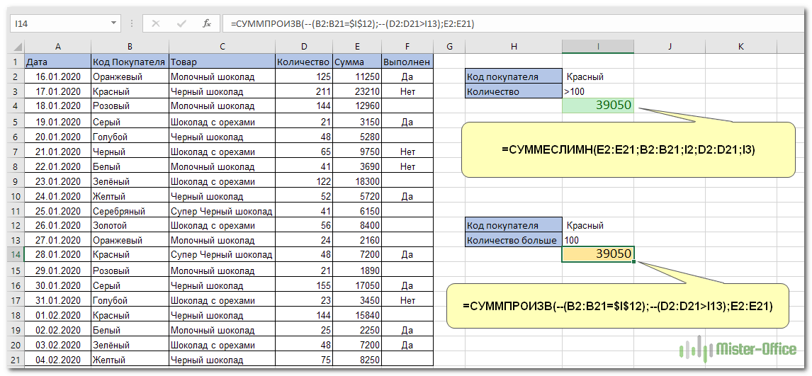
Разберем подробнее, как работает СУММПРОИЗВ():

=СУММПРОИЗВ(—(B2:B21=$I$12);—(D2:D21>I13);E2:E21)

Результатом вычисления B2:B21=$I$12 является массив

{ЛОЖЬ:ИСТИНА:ЛОЖЬ:ЛОЖЬ:ЛОЖЬ:ЛОЖЬ:ЛОЖЬ:ЛОЖЬ:ЛОЖЬ:ЛОЖЬ:ЛОЖЬ:ЛОЖЬ:ИСТИНА:ЛОЖЬ:ЛОЖЬ:ЛОЖЬ:ИСТИНА:ЛОЖЬ:ЛОЖЬ:ЛОЖЬ}.

ИСТИНА означает соответствие кода покупателя условию, т.е. слову Красный. Массив этот можно увидеть, выделив в строке формул B2:B21=$I$12, а затем нажав F9.

А что за странные знаки «минус» перед этими выражениями? Дело в том, что нам необходимы не эти логические выражения, а числа, чтобы их затем можно было перемножать и складывать. Если Эксель производит математическую операцию с логическим выражением, то он автоматически преобразует его в число. А знак минус означает умножение на -1. А если дважды умножить на -1, то число в результате не изменится. Это мы помним еще из школьной математики 😊

И в результате логический массив превратится в массив чисел {0:1:0:0:0:0:0:0:0:0:0:0:1:0:0:0:1:0:0:0}.

Результатом вычисления D2:D21>I13 является массив

{ИСТИНА:ИСТИНА:ИСТИНА:ЛОЖЬ:ЛОЖЬ:ЛОЖЬ:ЛОЖЬ:ИСТИНА:ЛОЖЬ:ЛОЖЬ:ЛОЖЬ:ЛОЖЬ:ЛОЖЬ:ЛОЖЬ:ИСТИНА:ЛОЖЬ:ИСТИНА:ЛОЖЬ:ЛОЖЬ:ЛОЖЬ}.

ИСТИНА соответствует ограничению «количество больше 100». Здесь мы также применяем двойное отрицание, чтобы преобразовать логические переменные в числа.

И, наконец, результатом вычисления В2:В13 является массив {11250:23210:12960:3150:5280:9750:3690:18300:5720:6150: 8400:2160:7200:1890:17050:3450:15840:2250:7200:8250}, т.е. просто числа из столбца E.

Результатом поэлементного умножения этих трех массивов является {0:23210:0:0:0:0:0:0:0:0:0:0:0:0:0:0:15840:0:0:0}. Суммируем эти произведения и получаем 39050.

Способ 3. Формула массива.

И еще один вариант расчета – применим формулу массива. В I14 запишем:

=СУММ((B2:B21=I12)*(D2:D21>I13)*(E2:E21))

Не забудьте в конце нажать комбинацию клавиш CTRL+SHIFT+ENTER, чтобы обозначить это выражение как формулу массива. Фигурные скобки в начале и в конце программа добавит автоматически. Вновь получим результат 39050.

Способ 4. Автофильтр.

Еще один альтернативный вариант – применение автофильтра. Для этого преобразуйте диапазон данных A1:F21 в «умную» таблицу. Напомню, что для этого в меню «Главная» выберите «Форматировать как таблицу». После этого добавьте в нее строку итогов (вкладка «Конструктор») и установите необходимые фильтры.

Без всяких формул итог по отфильтрованным строкам будет определён.

Как СУММЕСЛИМН работает с датами?

Если вы хотите отобрать и сложить какие-то показатели в определенном временном интервале на основе текущей даты, используйте функцию СЕГОДНЯ() в ваших ограничениях, как это показано ниже.

Следующая формула суммирует числа в столбце D, если соответствующая дата в столбце А попадает в последние 7 дней, включая сегодняшний день (предполагается, что сегодня 7 февраля):

=СУММЕСЛИМН(D2:D21;A2:A21;»<=»&СЕГОДНЯ();A2:A21;»>=»&СЕГОДНЯ()-6)

Замечание. Когда вы при составлении ограничения используете другую функцию Excel вместе с логическим оператором, нужно использовать амперсанд (&) для объединения всего выражения в виде текста, например «<=»&СЕГОДНЯ().

Аналогичным образом вы можете использовать функцию Excel СУММЕСЛИ для суммирования каких-то показателей в заданном диапазоне дат. Например, следующая формула также решит нашу задачу:

=СУММЕСЛИ(A2:A21;»>=»&СЕГОДНЯ()-6;D2:D21) — СУММЕСЛИ(A2:A21;»<=»&СЕГОДНЯ();D2:D21)

Однако СУММЕСЛИМН сложение делает гораздо проще и понятнее, не так ли?

Суммирование по пустым и непустым ячейкам.

При анализе отчетов и других данных вам часто может потребоваться суммировать данные, соответствующие пустым или непустым клеткам таблицы.

Критерии	Описание	Содержание
Пустые ячейки	«=»	Суммируйте числа, соответствующие пустым, которые не содержат абсолютно ничего — ни формулы, ни строки нулевой длины.	=СУММЕСЛИМН(C2:C10;A2:A10;»=»;B2:B10,»=») Суммируйте в C2:C10, если соответствующие ячейки в столбцах A и B абсолютно пусты.
	«»	Суммируйте числа, соответствующие «визуально» пустым, включая те, которые содержат пустые строки, возвращаемые какой-либо другой функцией Excel (например, ячейки с формулой вроде = «»).	=СУММЕСЛИМН(C2:C10;A2:A10;»»;B2:B10,»») Суммируйте в C2:C10 с теми же параметрами, что и в приведенной выше формуле, но с пустыми строками.
Непустые ячейки	«<>»	Суммируйте числа, соответствующие непустым, включая строки нулевой длины.	=СУММЕСЛИМН(C2:C10;A2:A10;»<>»;B2:B10,»<>») Суммируйте в C2: C10, если соответствующие ячейки в столбцах A и B не пусты, включая ячейки с пустыми строками.
		Суммируйте числа, соответствующие непустым, не включая строки нулевой длины.	=СУММ(C2:C10) — СУММЕСЛИМН(C2:C10;A2:A10;»»;B2:B10,»») или {=СУММ((C2:C10)(ДЛСТР(A2:A10)>0)(ДЛСТР(B2: B10)>0))} Если в столбцах A и B содержится текст ненулевой длины, тогда соответствующее число из C складывается. Внимание! Это формула массива! Фигурные скобки вводить не нужно!

А теперь давайте посмотрим, как вы можете использовать формулу СУММЕСЛИМН с «пустыми» и «непустыми» ячейками для реальных данных.

По покупателю «Красный» рассчитаем количество товара в невыполненных заказах. Для этого в столбце B ищем соответствующее название клиента, а в F – пустую ячейку. Если оба требования совпадают, складываем количество товара из столбца D.

=СУММЕСЛИМН(D2:D21;F2:F21;»»;B2:B21;»Красный»)

или

=СУММЕСЛИМН(D2:D21;F2:F21;»=»;B2:B21;»Красный»)

Каждое из этих выражений дает верный результат – 144 единицы в заказе от 4 февраля.

Сумма нескольких условий.

А теперь давайте рассчитаем общую стоимость выполненных заказов по двум товарам.

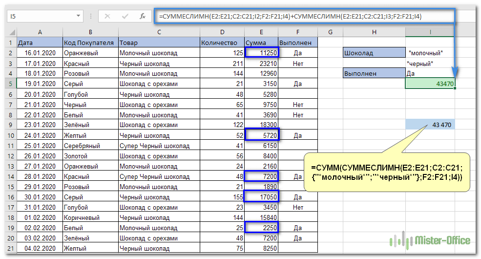
Если мы просто добавим второй критерий в I3, и вместо I2 используем область I2:I3, то расчет будет неверным, поскольку в C2:C21 будем искать товар, в названии которого есть И «черный», И «молочный» одновременно. Ведь таких просто нет.

Поэтому первый вариант расчета таков:

=СУММЕСЛИМН(E2:E21;C2:C21;I2;F2:F21;I4)+СУММЕСЛИМН(E2:E21;C2:C21;I3;F2:F21;I4)

Просто складываем выполненные заказы сначала по первому, а затем по второму наименованию.

Второй вариант: используем элемент массива критериев и функцию СУММ.

=СУММ(СУММЕСЛИМН(E2:E21;C2:C21;{«*молочный*»;»*черный*»};F2:F21;I4))

Как видите, результаты получены одинаковые. Выбирайте способ, который будет для вас проще и понятнее.

Ещё примеры расчета суммы:

Источник

На чтение 2 мин

Функция СУММЕСЛИМН (SUMIFS) в Excel используется для суммирования значений по нескольким критериям. Если вы хотите суммировать значения по одному критерию, то лучше использовать функцию SUMIF (СУММЕСЛИ).

Содержание

Что возвращает функция
Синтаксис
Аргументы функции
Дополнительная информация
Примеры использования функции СУММЕСЛИМН в Excel

Что возвращает функция

Возвращает сумму чисел по нескольким критериям.

Больше лайфхаков в нашем Telegram Подписаться

Синтаксис

=SUMIFS(sum_range, criteria_range1, criteria1, [criteria_range2, critertia2],…) — английская версия

=СУММЕСЛИМН(диапазон_суммирования; диапазон_условия1; условие1; [диапазон_условия2; условие2]; …) — русская версия

Аргументы функции

sum_range (диапазон_суммирования) — это диапазон данных, по которым будут вычисляться условия указанных вами критериев для суммирования данных;
criteria_range1 (диапазон_условия1), сriteria1 (условие1) — диапазон, в котором проверяется первое условие функции. Criteria_range1 (диапазон_условия1) и criteria1(условие1) составляют пару, определяющую, к какому диапазону применяется определенное условие при поиске. Соответствующие значения найденных в этом диапазоне ячеек суммируются в пределах аргумента sum_range (диапазон_суммирования).
[criteria_range2], criteria2 ([диапазон_условия2], условие 2) — (опционально) — второй диапазон критериев, по которым будут вычисляться данные;

Дополнительная информация

Суммирование значений в функции производится на основе нескольких критериев;
Пустые и текстовые ячейки игнорируются в аргументе sum_range (диапазон_суммирования);
Критерием могут служить числа, выражения, ссылка на ячейку, текст или формула;
Критерий, указанный в текстовом или логическом/математическом формате (=,+,-,/,*) должны быть указаны в двойных кавычках;
В качестве критерия могут использоваться подстановочные знаки (*);
Критерий не может быть больше чем 255 символов по длине;
Ячейки в аргументе sum_range (диапазон_суммирования) суммируются только при выполнении всех условий, заданных в формуле;
Если среди значений аргумента sum_range (диапазон_суммирования) указано логическое значение TRUE или FALSE, то они подразумевают значения «1» и «0» соответственно;
Диапазон аргументов sum_range (диапазон_суммирования) и всех критериев должны совпадать.

Примеры использования функции СУММЕСЛИМН в Excel

Источник

Sums all data based on multiple criteria

What is the SUMIFS Function in Excel?

We all know the SUMIF function allows us to sum the data given based on associated criteria within the same data. However, the SUMIFs Function[1] in Excel allows applying multiple criteria.

Formula used for the SUMIFS Function in Excel

“SUMIFS ( sum_range, criteria_range1, criteria1, [criteria_range2, criteria2, criteria_range3, criteria3, … criteria_range_n, criteria_n] )”

Where:

Sum_range = Cells to add

Criteria_range1 = Range of cells that we want to apply criteria1 against

Criteria1 = Used to determine which cells to add. Criteria1 is applied against criteria_range1.

Criteria_range2, criteria2, … = The additional ranges along with their associated criteria.

The SUMIFS Function in Excel allows us to enter up to 127 range/criteria pairs for this formula. Remember:

SUMIFS will return a numeric value.
Rows and columns should be the same in the criteria_range argument and the sum_range argument.

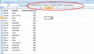
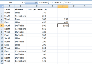
Let’s take an example to understand it. Suppose we use data about flowers and their cost per dozen for different regions. If I need to find out the total cost for Carnations for the South region, I can do it in the following manner:

Similarly, if I wish to find out the total cost of Daffodils for the North region, I can use the same formula.

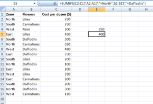
Suppose I wish to find out the total cost of flowers for the East region, the formula to be used would be:

The SUMIFS function can use comparison operators like ‘=’, ‘>’, ‘<‘. If we wish to use these operators, we can apply them to an actual sum range or any of the criteria ranges. Also, we can create comparison operators using them:

‘<=’ (less than or equal to)
‘>=’ (greater than or equal to)
‘<>’ (less than or greater than/not equal to)

Let’s take an example to understand this in detail.

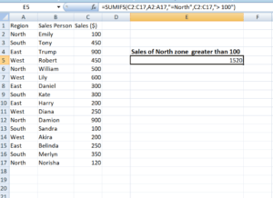
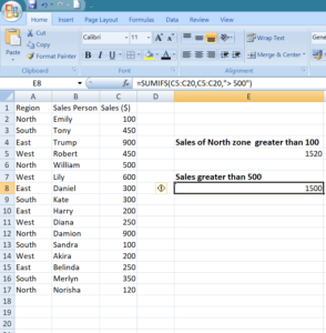
Using the sales figures per region of different salespersons, I wish to find out the:

Sales of North region greater than 100
Sales greater than 500

I can use the abovementioned operators as follows:

Sales of North region greater than 100

Sales greater than 500

To learn more, launch our free Excel crash course now!

Use of wildcards

Wildcard characters such as ‘*’ and ‘?’ can be used within the criteria argument when using the SUMIFS function. Using these wildcards will help us in finding matches that are a similar but not accurate match.

Asterisk (*) – It matches any sequence of characters. It can be used after, before or surrounding criteria to allow partial search criteria to be used.

For example, if I apply the following criteria in SUMIFS function:

N* – It implies all cells in the range that start with N
*N – It implies all cells in the range that ends with N
*N* – Cells that contain N

Question mark (?) – It matches any single character. Suppose I apply N?r as the criteria. Here “?” will take the place of a single character. N?r will match with North, Nor, etc. However, it will not take into consideration Name.

What if the given data contain an asterisk or an actual question mark?

In this case, we can use “tilde (~)”. We need to type “~” in front of the question mark in that scenario.

Using named ranges with SUMIFS Function

Named range is the descriptive name of a collection of cells or range in a worksheet. We can use named ranges while using the SUMIFS function.

To learn more, launch our free Excel crash course now!

SUMIF vs. SUMIFS

When using SUMIF, we can evaluate only one condition, whereas different criteria can be evaluated under SUMIFS formula. This is the primary difference between the two Excel functions.
SUMIFS is available from MS Excel 2007.
The SUMIF function can be only used for adding a single continuous range based on a single specified range with a single criterion, whereas, SUMIFS can be applied over multiple continuous ranges.

Free Excel Course

Don’t forget to check out CFI’s Free Excel Crash Course to learn more about functions and develop your overall Excel skills. Become a successful financial analyst by learning how to create sophisticated financial analysis and financial modeling.

Additional Resources

Thank you for reading CFI’s guide on the SUMIFS Function in Excel. To learn more, check out these additional CFI resources:

Excel Functions for Finance
Advanced Excel Formulas Course
Advanced Excel Formulas You Must Know
Excel Shortcuts for PC and Mac
See all Excel resources

Article Sources

SUMIFS Function

Источник

Syntax

Examples

Common Problems

Best practices

Need more help?

See Also

Need more help?

What to Know

Entering the Tutorial Data

The SUMIFS Function’s Syntax

Starting the SUMIFS Function

Entering the Sum_range Argument

Tutorial Steps

Entering the Criteria_range1 Argument

Tutorial Steps

Entering the Criteria1 Argument

Tutorial Steps

How Cell References Increase SUMIFS Versatility

Entering the Criteria_range2 Argument

Entering the Criteria2 Argument

Adding the Search Criteria and Completing the Tutorial

How the SUMIFS Function Works

The SUMIFS Function’s Arguments

Как работает СУММЕСЛИМН?

Использование СУММЕСЛИМН и СУММЕСЛИ в Excel — что нужно запомнить?

1. Порядок аргументов

2. Диапазон суммирования и область критериев должны быть одинакового размера

Суммирование с множеством условий.

Использование операторов сравнения.

Способ 2. Используем функцию СУММПРОИЗВ.

Способ 3. Формула массива.

Способ 4. Автофильтр.

Как СУММЕСЛИМН работает с датами?

Суммирование по пустым и непустым ячейкам.

Что возвращает функция

Синтаксис

Аргументы функции

Дополнительная информация

Примеры использования функции СУММЕСЛИМН в Excel

What is the SUMIFS Function in Excel?

Formula used for the SUMIFS Function in Excel

Sales of North region greater than 100

Sales greater than 500

Use of wildcards

Using named ranges with SUMIFS Function

SUMIF vs. SUMIFS

Free Excel Course

Additional Resources

Article Sources