
Содержание
- Манипуляции с именованными областями
- Создание именованного диапазона
- Операции с именованными диапазонами
- Управление именованными диапазонами
- Вопросы и ответы

Одним из инструментов, который упрощает работу с формулами и позволяет оптимизировать работу с массивами данных, является присвоение этим массивам наименования. Таким образом, если вы хотите сослаться на диапазон однородных данных, то не нужно будет записывать сложную ссылку, а достаточно указать простое название, которым вы сами ранее обозначили определенный массив. Давайте выясним основные нюансы и преимущества работы с именованными диапазонами.
Манипуляции с именованными областями
Именованный диапазон — это область ячеек, которой пользователем присвоено определенное название. При этом данное наименование расценивается Excel, как адрес указанной области. Оно может использоваться в составе формул и аргументов функций, а также в специализированных инструментах Excel, например, «Проверка вводимых значений».
Существуют обязательные требования к наименованию группы ячеек:
- В нём не должно быть пробелов;
- Оно обязательно должно начинаться с буквы;
- Его длина не должна быть больше 255 символов;
- Оно не должно быть представлено координатами вида A1 или R1C1;
- В книге не должно быть одинаковых имен.
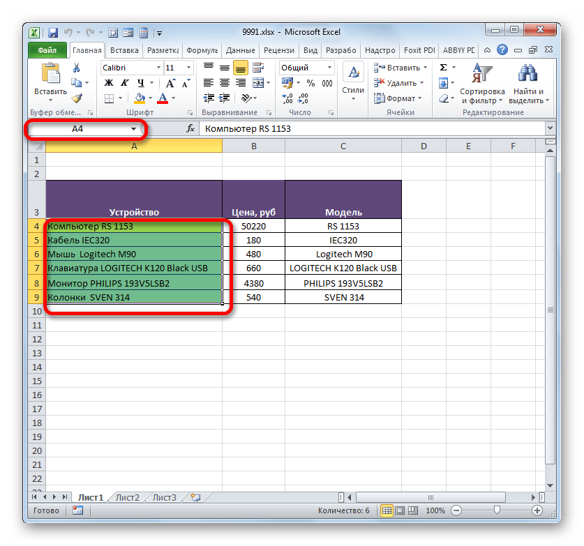
Наименование области ячеек можно увидеть при её выделении в поле имен, которое размещено слева от строки формул.
В случае, если наименование диапазону не присвоено, то в вышеуказанном поле при его выделении отображается адрес левой верхней ячейки массива.
Создание именованного диапазона
Прежде всего, узнаем, как создать именованный диапазон в Экселе.
- Самый быстрый и простой вариант присвоения названия массиву – это записать его в поле имен после выделения соответствующей области. Итак, выделяем массив и вводим в поле то название, которое считаем нужным. Желательно, чтобы оно легко запоминалось и отвечало содержимому ячеек. И, безусловно, необходимо, чтобы оно отвечало обязательным требованиям, которые были изложены выше.
- Для того, чтобы программа внесла данное название в собственный реестр и запомнила его, жмем по клавише Enter. Название будет присвоено выделенной области ячеек.


Выше был назван самый быстрый вариант наделения наименованием массива, но он далеко не единственный. Эту процедуру можно произвести также через контекстное меню
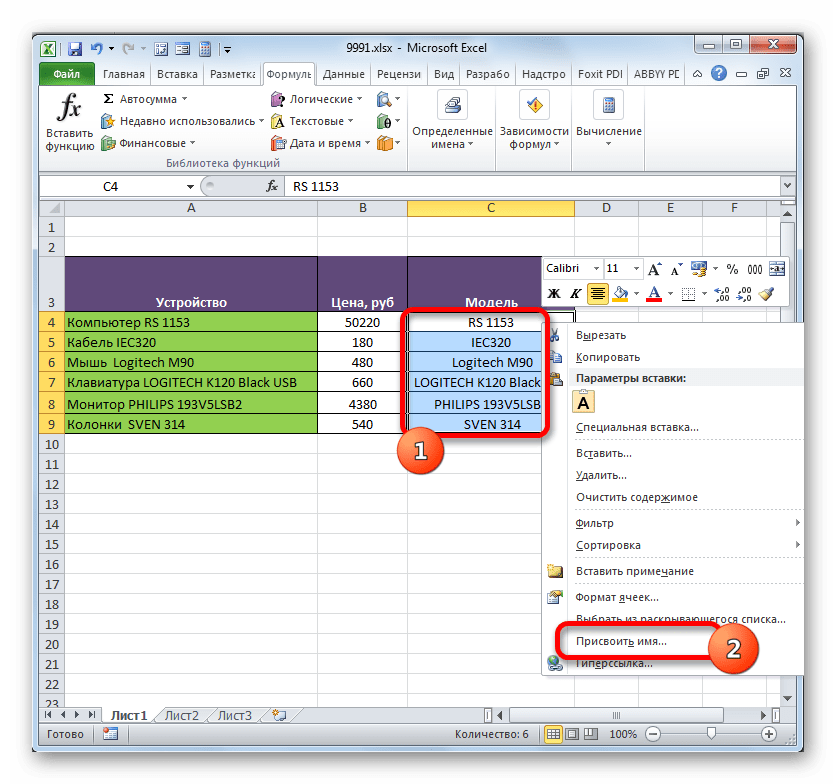
- Выделяем массив, над которым требуется выполнить операцию. Клацаем по выделению правой кнопкой мыши. В открывшемся списке останавливаем выбор на варианте «Присвоить имя…».
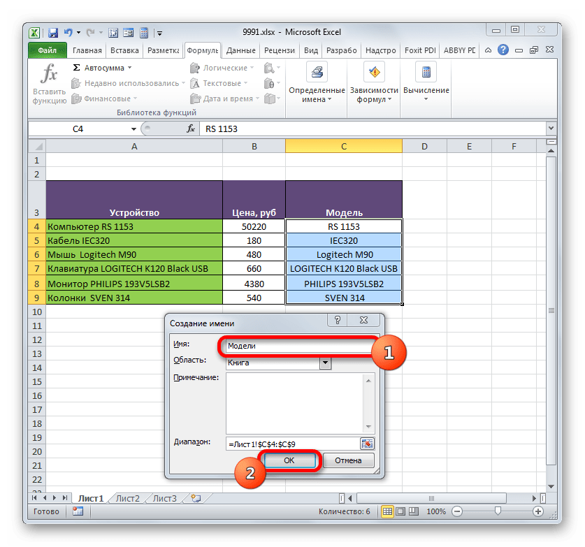
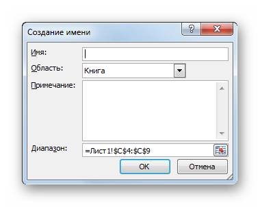
- Открывается окошко создания названия. В область «Имя» следует вбить наименование в соответствии с озвученными выше условиями. В области «Диапазон» отображается адрес выделенного массива. Если вы провели выделение верно, то вносить изменения в эту область не нужно. Жмем по кнопке «OK».
- Как можно видеть в поле имён, название области присвоено успешно.

Ещё один вариант выполнения указанной задачи предусматривает использование инструментов на ленте.
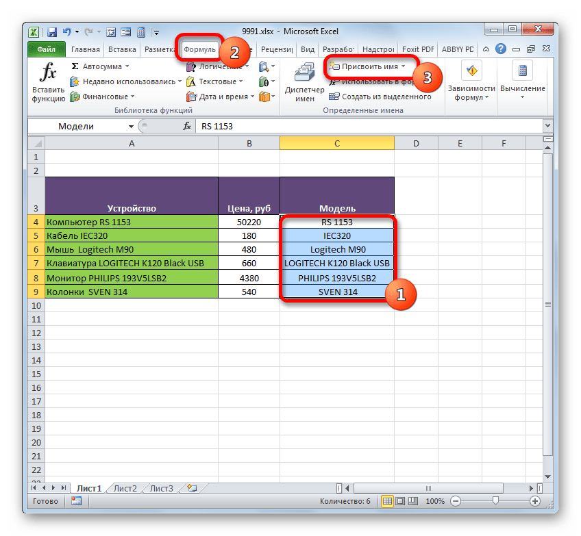
- Выделяем область ячеек, которую требуется преобразовать в именованную. Передвигаемся во вкладку «Формулы». В группе «Определенные имена» производим клик по значку «Присвоить имя».
- Открывается точно такое же окно присвоения названия, как и при использовании предыдущего варианта. Все дальнейшие операции выполняются абсолютно аналогично.
Последний вариант присвоения названия области ячеек, который мы рассмотрим, это использование Диспетчера имен.
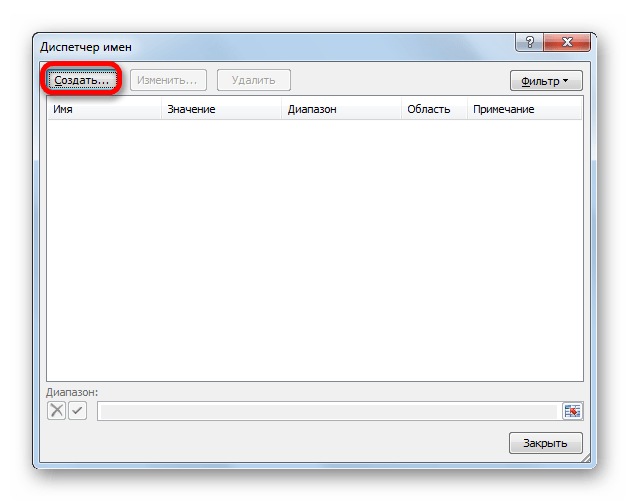
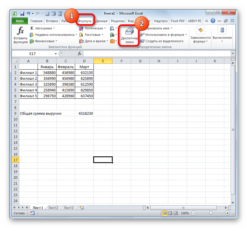
- Выделяем массив. На вкладке «Формулы», клацаем по крупному значку «Диспетчер имен», расположенному всё в той же группе «Определенные имена». Или же можно вместо этого применить нажатие сочетания клавиш Ctrl+F3.
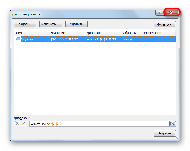
- Активируется окно Диспетчера имён. В нем следует нажать на кнопку «Создать…» в верхнем левом углу.
- Затем запускается уже знакомое окошко создания файлов, где нужно провести те манипуляции, о которых шёл разговор выше. То имя, которое будет присвоено массиву, отобразится в Диспетчере. Его можно будет закрыть, нажав на стандартную кнопку закрытия в правом верхнем углу.

Урок: Как присвоить название ячейке в Экселе
Операции с именованными диапазонами
Как уже говорилось выше, именованные массивы могут использоваться во время выполнения различных операций в Экселе: формулы, функции, специальные инструменты. Давайте на конкретном примере рассмотрим, как это происходит.
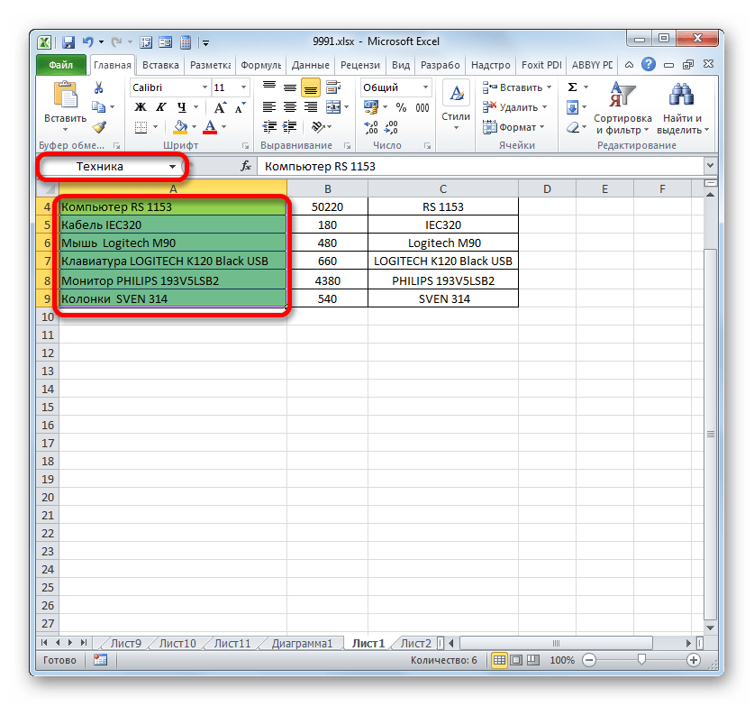
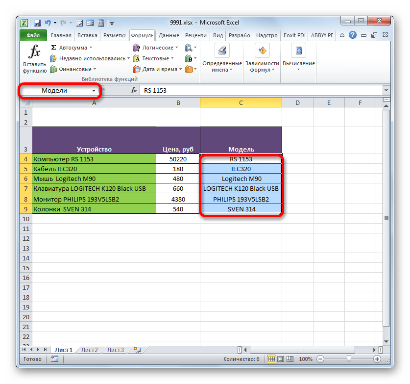
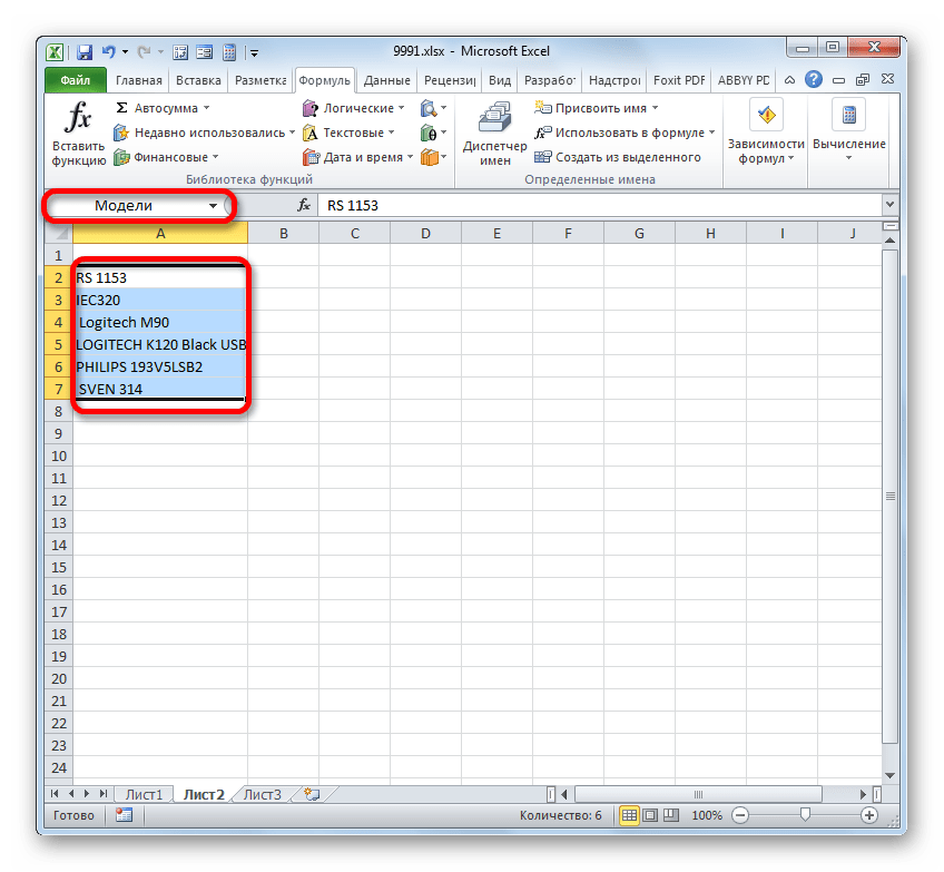
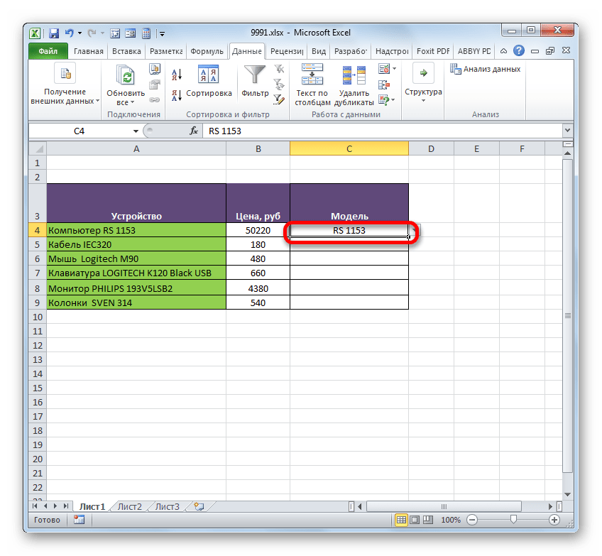
На одном листе у нас перечень моделей компьютерной техники. У нас стоит задача на втором листе в таблице сделать выпадающий список из данного перечня.
- Прежде всего, на листе со списком присваиваем диапазону наименование любым из тех способов, о которых шла речь выше. В итоге, при выделении перечня в поле имён у нас должно отображаться наименование данного массива. Пусть это будет наименование «Модели».
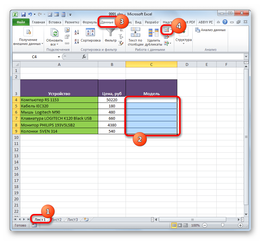
- После этого перемещаемся на лист, где находится таблица, в которой нам предстоит создать выпадающий список. Выделяем область в таблице, в которую планируем внедрить выпадающий список. Перемещаемся во вкладку «Данные» и щелкаем по кнопке «Проверка данных» в блоке инструментов «Работа с данными» на ленте.
- В запустившемся окне проверки данных переходим во вкладку «Параметры». В поле «Тип данных» выбираем значение «Список». В поле «Источник» в обычном случае нужно либо вручную вписать все элементы будущего выпадающего списка, либо дать ссылку на их перечень, если он расположен в документе. Это не очень удобно, особенно, если перечень располагается на другом листе. Но в нашем случае все намного проще, так как мы соответствующему массиву присвоили наименование. Поэтому просто ставим знак «равно» и записываем это название в поле. Получается следующее выражение:
=МоделиЖмем по «OK».
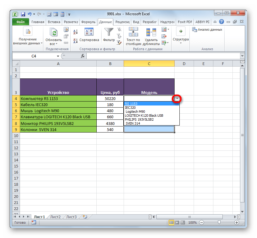
- Теперь при наведении курсора на любую ячейку диапазона, к которой мы применили проверку данных, справа от неё появляется треугольник. При нажатии на этот треугольник открывается список вводимых данных, который подтягивается из перечня на другом листе.
- Нам просто остается выбрать нужный вариант, чтобы значение из списка отобразилось в выбранной ячейке таблицы.

Именованный диапазон также удобно использовать в качестве аргументов различных функций. Давайте взглянем, как это применяется на практике на конкретном примере.
Итак, мы имеем таблицу, в которой помесячно расписана выручка пяти филиалов предприятия. Нам нужно узнать общую выручку по Филиалу 1, Филиалу 3 и Филиалу 5 за весь период, указанный в таблице.
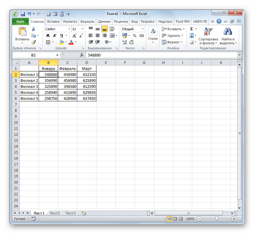
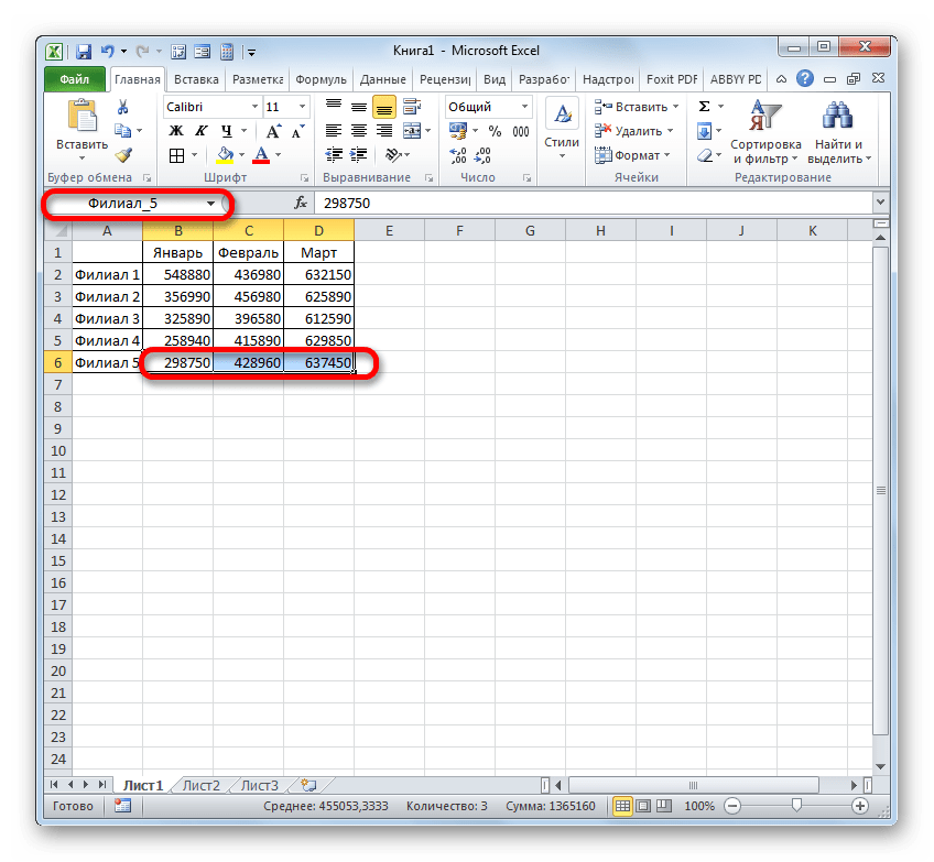
- Прежде всего, каждой строке соответствующего филиала в таблице присвоим название. Для Филиала 1 выделяем область с ячейками, в которых содержатся данные о выручке по нему за 3 месяца. После выделения в поле имен пишем наименование «Филиал_1» (не забываем, что название не может содержать пробел) и щелкаем по клавише Enter. Наименование соответствующей области будет присвоено. При желании можно использовать любой другой вариант присвоения наименования, о котором шел разговор выше.
- Таким же образом, выделяя соответствующие области, даем названия строкам и других филиалов: «Филиал_2», «Филиал_3», «Филиал_4», «Филиал_5».
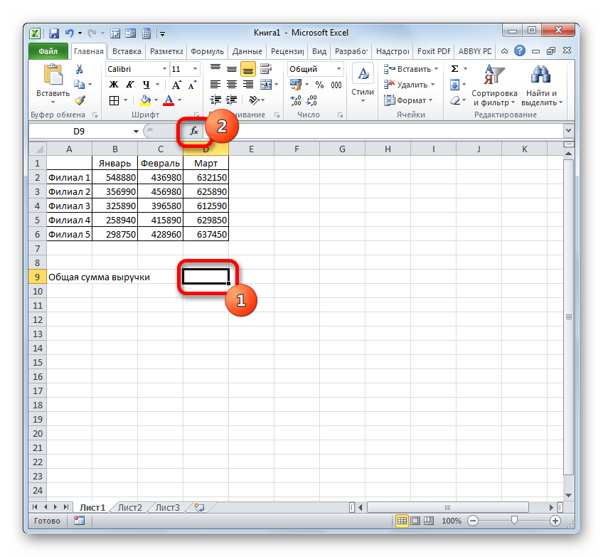
- Выделяем элемент листа, в который будет выводиться итог суммирования. Клацаем по иконке «Вставить функцию».
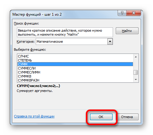
- Инициируется запуск Мастера функций. Производим перемещение в блок «Математические». Останавливаем выбор из перечня доступных операторов на наименовании «СУММ».
- Происходит активация окошка аргументов оператора СУММ. Данная функция, входящая в группу математических операторов, специально предназначена для суммирования числовых значений. Синтаксис представлен следующей формулой:
=СУММ(число1;число2;…)Как нетрудно понять, оператор суммирует все аргументы группы «Число». В виде аргументов могут применяться, как непосредственно сами числовые значения, так и ссылки на ячейки или диапазоны, где они расположены. В случае применения массивов в качестве аргументов используется сумма значений, которая содержится в их элементах, подсчитанная в фоновом режиме. Можно сказать, что мы «перескакиваем», через действие. Именно для решения нашей задачи и будет использоваться суммирование диапазонов.
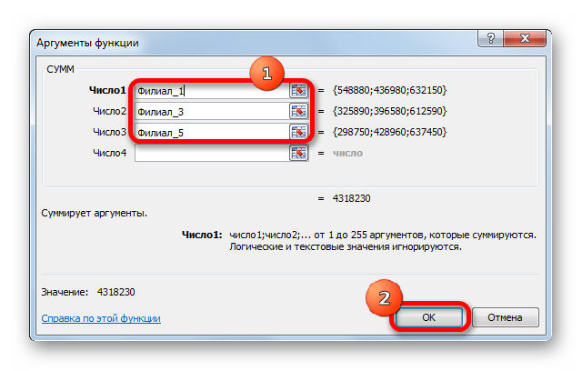
Всего оператор СУММ может насчитывать от одного до 255 аргументов. Но в нашем случае понадобится всего три аргумента, так как мы будет производить сложение трёх диапазонов: «Филиал_1», «Филиал_3» и «Филиал_5».
Итак, устанавливаем курсор в поле «Число1». Так как мы дали названия диапазонам, которые требуется сложить, то не нужно ни вписывать координаты в поле, ни выделять соответствующие области на листе. Достаточно просто указать название массива, который подлежит сложению: «Филиал_1». В поля «Число2» и «Число3» соответственно вносим запись «Филиал_3» и «Филиал_5». После того, как вышеуказанные манипуляции были сделаны, клацаем по «OK».
- Результат вычисления выведен в ячейку, которая была выделена перед переходом в Мастер функций.

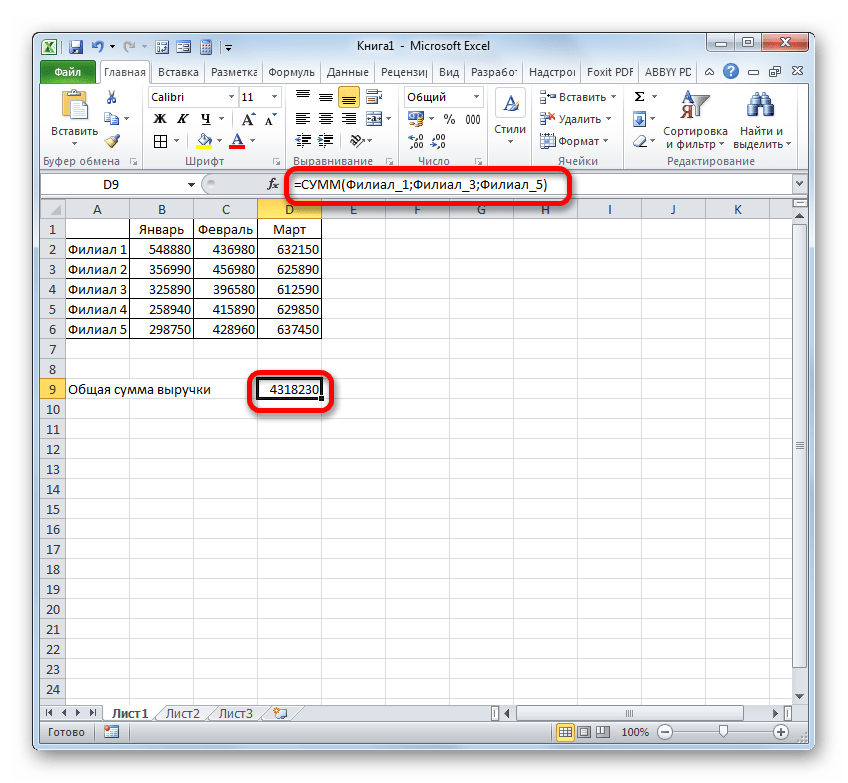
Как видим, присвоение названия группам ячеек в данном случае позволило облегчить задачу сложения числовых значений, расположенных в них, в сравнении с тем, если бы мы оперировали адресами, а не наименованиями.
Конечно, эти два примера, которые мы привели выше, показывают далеко не все преимущества и возможности применения именованных диапазонов при использовании их в составе функций, формул и других инструментов Excel. Вариантов использования массивов, которым было присвоено название, неисчислимое множество. Тем не менее, указанные примеры все-таки позволяют понять основные преимущества присвоения наименования областям листа в сравнении с использованием их адресов.
Урок: Как посчитать сумму в Майкрософт Эксель
Управление именованными диапазонами
Управлять созданными именованными диапазонами проще всего через Диспетчер имен. При помощи данного инструмента можно присваивать имена массивам и ячейкам, изменять существующие уже именованные области и ликвидировать их. О том, как присвоить имя с помощью Диспетчера мы уже говорили выше, а теперь узнаем, как производить в нем другие манипуляции.
- Чтобы перейти в Диспетчер, перемещаемся во вкладку «Формулы». Там следует кликнуть по иконке, которая так и называется «Диспетчер имен». Указанная иконка располагается в группе «Определенные имена».
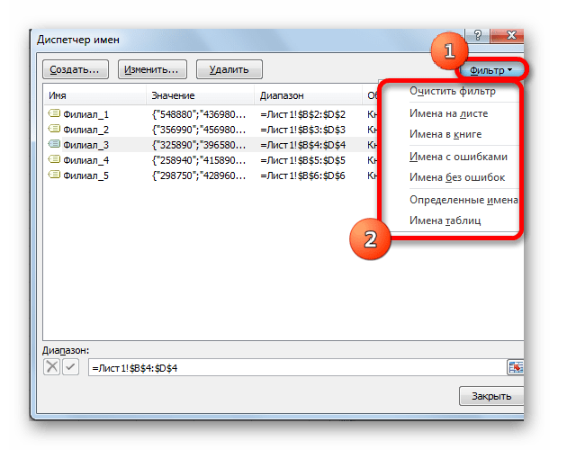
- После перехода в Диспетчер для того, чтобы произвести необходимую манипуляцию с диапазоном, требуется найти его название в списке. Если перечень элементов не очень обширный, то сделать это довольно просто. Но если в текущей книге располагается несколько десятков именованных массивов или больше, то для облегчения задачи есть смысл воспользоваться фильтром. Клацаем по кнопке «Фильтр», размещенной в правом верхнем углу окна. Фильтрацию можно выполнять по следующим направлениям, выбрав соответствующий пункт открывшегося меню:
- Имена на листе;
- в книге;
- с ошибками;
- без ошибок;
- Определенные имена;
- Имена таблиц.
Для того, чтобы вернутся к полному перечню наименований, достаточно выбрать вариант «Очистить фильтр».
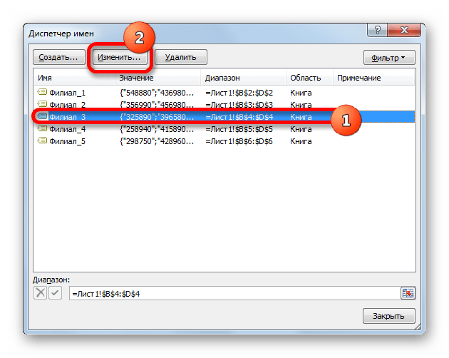
- Для изменения границ, названия или других свойств именованного диапазона следует выделить нужный элемент в Диспетчере и нажать на кнопку «Изменить…».
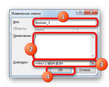
- Открывается окно изменение названия. Оно содержит в себе точно такие же поля, что и окно создания именованного диапазона, о котором мы говорили ранее. Только на этот раз поля будут заполнены данными.
В поле «Имя» можно сменить наименование области. В поле «Примечание» можно добавить или отредактировать существующее примечание. В поле «Диапазон» можно поменять адрес именованного массива. Существует возможность сделать, как применив ручное введение требуемых координат, так и установив курсор в поле и выделив соответствующий массив ячеек на листе. Его адрес тут же отобразится в поле. Единственное поле, значения в котором невозможно отредактировать – «Область».
После того, как редактирование данных окончено, жмем на кнопку «OK».
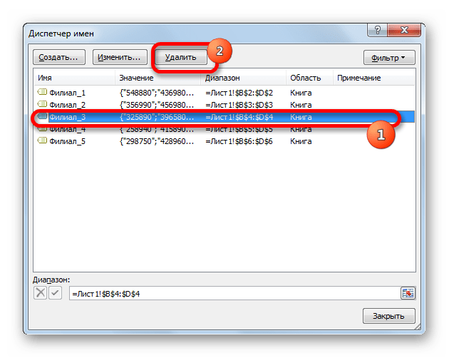
Также в Диспетчере при необходимости можно произвести процедуру удаления именованного диапазона. При этом, естественно, будет удаляться не сама область на листе, а присвоенное ей название. Таким образом, после завершения процедуры к указанному массиву можно будет обращаться только через его координаты.
Это очень важно, так как если вы уже применяли удаляемое наименование в какой-то формуле, то после удаления названия данная формула станет ошибочной.
- Чтобы провести процедуру удаления, выделяем нужный элемент из перечня и жмем на кнопку «Удалить».
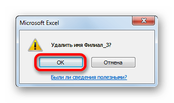
- После этого запускается диалоговое окно, которое просит подтвердить свою решимость удалить выбранный элемент. Это сделано во избежание того, чтобы пользователь по ошибке не выполнил данную процедуру. Итак, если вы уверены в необходимости удаления, то требуется щелкнуть по кнопке «OK» в окошке подтверждения. В обратном случае жмите по кнопке «Отмена».
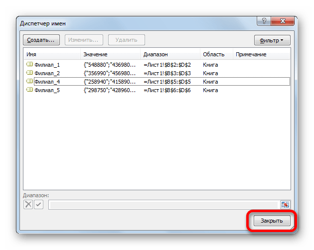
- Как видим, выбранный элемент был удален из перечня Диспетчера. Это означает, что массив, к которому он был прикреплен, утратил наименование. Теперь он будет идентифицироваться только по координатам. После того, как все манипуляции в Диспетчере завершены, клацаем по кнопке «Закрыть», чтобы завершить работу в окне.
Применение именованного диапазона способно облегчить работу с формулами, функциями и другими инструментами Excel. Самими именованными элементами можно управлять (изменять и удалять) при помощи специального встроенного Диспетчера.
What’s in the name?
If you are working with Excel spreadsheets, it could mean a lot of time saving and efficiency.
In this tutorial, you’ll learn how to create Named Ranges in Excel and how to use it to save time.
Named Ranges in Excel – An Introduction
If someone has to call me or refer to me, they will use my name (instead of saying a male is staying in so and so place with so and so height and weight).
Right?
Similarly, in Excel, you can give a name to a cell or a range of cells.
Now, instead of using the cell reference (such as A1 or A1:A10), you can simply use the name that you assigned to it.
For example, suppose you have a data set as shown below:
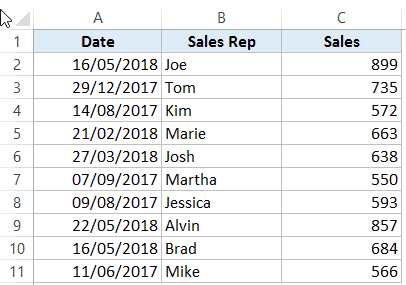
In this data set, if you have to refer to the range that has the Date, you will have to use A2:A11 in formulas. Similarly, for Sales Rep and Sales, you will have to use B2:B11 and C2:C11.
While it’s alright when you only have a couple of data points, but in case you huge complex data sets, using cell references to refer to data could be time-consuming.
Excel Named Ranges makes it easy to refer to data sets in Excel.
You can create a named range in Excel for each data category, and then use that name instead of the cell references. For example, dates can be named ‘Date’, Sales Rep data can be named ‘SalesRep’ and sales data can be named ‘Sales’.

You can also create a name for a single cell. For example, if you have the sales commission percentage in a cell, you can name that cell as ‘Commission’.
Benefits of Creating Named Ranges in Excel
Here are the benefits of using named ranges in Excel.
Use Names instead of Cell References
When you create Named Ranges in Excel, you can use these names instead of the cell references.
For example, you can use =SUM(SALES) instead of =SUM(C2:C11) for the above data set.
Have a look at ṭhe formulas listed below. Instead of using cell references, I have used the Named Ranges.
- Number of sales with value more than 500: =COUNTIF(Sales,”>500″)
- Sum of all the sales done by Tom: =SUMIF(SalesRep,”Tom”,Sales)
- Commission earned by Joe (sales by Joe multiplied by commission percentage):
=SUMIF(SalesRep,”Joe”,Sales)*Commission
You would agree that these formulas are easy to create and easy to understand (especially when you share it with someone else or revisit it yourself.
No Need to Go Back to the Dataset to Select Cells
Another significant benefit of using Named Ranges in Excel is that you don’t need to go back and select the cell ranges.
You can just type a couple of alphabets of that named range and Excel will show the matching named ranges (as shown below):

Named Ranges Make Formulas Dynamic
By using Named Ranges in Excel, you can make Excel formulas dynamic.
For example, in the case of sales commission, instead of using the value 2.5%, you can use the Named Range.
Now, if your company later decides to increase the commission to 3%, you can simply update the Named Range, and all the calculation would automatically update to reflect the new commission.
How to Create Named Ranges in Excel
Here are three ways to create Named Ranges in Excel:
Method #1 – Using Define Name
Here are the steps to create Named Ranges in Excel using Define Name:
This will create a Named Range SALESREP.
Method #2: Using the Name Box
- Select the range for which you want to create a name (do not select headers).
- Go to the Name Box on the left of Formula bar and Type the name of the with which you want to create the Named Range.

- Note that the Name created here will be available for the entire Workbook. If you wish to restrict it to a worksheet, use Method 1.
Method #3: Using Create From Selection Option
This is the recommended way when you have data in tabular form, and you want to create named range for each column/row.
For example, in the dataset below, if you want to quickly create three named ranges (Date, Sales_Rep, and Sales), then you can use the method shown below.
Here are the steps to quickly create named ranges from a dataset:
This will create three Named Ranges – Date, Sales_Rep, and Sales.
Note that it automatically picks up names from the headers. If there are any space between words, it inserts an underscore (as you can’t have spaces in named ranges).
Naming Convention for Named Ranges in Excel
There are certain naming rules you need to know while creating Named Ranges in Excel:
- The first character of a Named Range should be a letter and underscore character(_), or a backslash(). If it’s anything else, it will show an error. The remaining characters can be letters, numbers, special characters, period, or underscore.
- You can not use names that also represent cell references in Excel. For example, you can’t use AB1 as it is also a cell reference.
- You can’t use spaces while creating named ranges. For example, you can’t have Sales Rep as a named range. If you want to combine two words and create a Named Range, use an underscore, period or uppercase characters to create it. For example, you can have Sales_Rep, SalesRep, or SalesRep.
- While creating named ranges, Excel treats uppercase and lowercase the same way. For example, if you create a named range SALES, then you will not be able to create another named range such as ‘sales’ or ‘Sales’.
- A Named Range can be up to 255 characters long.
Too Many Named Ranges in Excel? Don’t Worry
Sometimes in large data sets and complex models, you may end up creating a lot of Named Ranges in Excel.
What if you don’t remember the name of the Named Range you created?
Don’t worry – here are some useful tips.
Getting the Names of All the Named Ranges
Here are the steps to get a list of all the named ranges you created:
This will give you a list of all the Named Ranges in that workbook. To use a named range (in formulas or a cell), double click on it.

Displaying the Matching Named Ranges
- If you have some idea about the Name, type a few initial characters, and Excel will show a drop down of the matching names.


How to Edit Named Ranges in Excel
If you have already created a Named Range, you can edit it using the following steps:
Useful Named Range Shortcuts (the Power of F3)
Here are some useful keyboard shortcuts that will come handy when you are working with Named Ranges in Excel:
- To get a list of all the Named Ranges and pasting it in Formula: F3
- To create new name using Name Manager Dialogue Box: Control + F3
- To create Named Ranges from Selection: Control + Shift + F3
Creating Dynamic Named Ranges in Excel
So far in this tutorial, we have created static Named Ranges.
This means that these Named Ranges would always refer to the same dataset.
For example, if A1:A10 has been named as ‘Sales’, it would always refer to A1:A10.
If you add more sales data, then you would have to manually go and update the reference in the named range.
In the world of ever-expanding data sets, this may end up taking up a lot of your time. Every time you get new data, you may have to update the Named Ranges in Excel.
To tackle this issue, we can create Dynamic Named Ranges in Excel that would automatically account for additional data and include it in the existing Named Range.
For example, For example, if I add two additional sales data points, a dynamic named range would automatically refer to A1:A12.
This kind of Dynamic Named Range can be created by using Excel INDEX function. Instead of specifying the cell references while creating the Named Range, we specify the formula. The formula automatically updated when the data is added or deleted.
Let’s see how to create Dynamic Named Ranges in Excel.
Suppose we have the sales data in cell A2:A11.

Here are the steps to create Dynamic Named Ranges in Excel:
-
- Go to the Formula tab and click on Define Name.

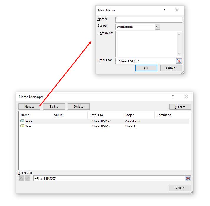
- In the New Name dialogue box type the following:
- Name: Sales
- Scope: Workbook
- Refers to: =$A$2:INDEX($A$2:$A$100,COUNTIF($A$2:$A$100,”<>”&””))

- Click OK.
- Go to the Formula tab and click on Define Name.


Done!
You now have a dynamic named range with the name ‘Sales’. This would automatically update whenever you add data to it or remove data from it.
How does Dynamic Named Ranges Work?
To explain how this work, you need to know a bit more about Excel INDEX function.
Most people use INDEX to return a value from a list based on the row and column number.
But the INDEX function also has another side to it.
It can be used to return a cell reference when it is used as a part of a cell reference.
For example, here is the formula that we have used to create a dynamic named range:
=$A$2:INDEX($A$2:$A$100,COUNTIF($A$2:$A$100,"<>"&""))
INDEX($A$2:$A$100,COUNTIF($A$2:$A$100,”<>”&””) –> This part of the formula is expected to return a value (which would be the 10th value from the list, considering there are ten items).
However, when used in front of a reference (=$A$2:INDEX($A$2:$A$100,COUNTIF($A$2:$A$100,”<>”&””))) it returns the reference to the cell instead of the value.
Hence, here it returns =$A$2:$A$11
If we add two additional values to the sales column, it would then return =$A$2:$A$13
When you add new data to the list, Excel COUNTIF function returns the number of non-blank cells in the data. This number is used by the INDEX function to fetch the cell reference of the last item in the list.
Note:
- This would only work if there are no blank cells in the data.
- In the example taken above, I have assigned a large number of cells (A2:A100) for the Named Range formula. You can adjust this based on your data set.
You can also use OFFSET function to create a Dynamic Named Ranges in Excel, however, since OFFSET function is volatile, it may lead a slow Excel workbook. INDEX, on the other hand, is semi-volatile, which makes it a better choice to create Dynamic Named Ranges in Excel.
You may also like the following Excel resources:
- Free Excel Templates.
- Free Online Excel Training (7-Part Online Video Course).
- Useful Excel Macro Code Examples.
- 10 Advanced Excel VLOOKUP Examples.
- Creating a Drop Down List in Excel.
- Creating a Named Range in Google Sheets.
- How to Reference Another Sheet or Workbook in Excel
- How to Delete Named Range in Excel?
We can use the name for the cell Ranges instead of the cell reference (such as A1 or A1:A10). We can create a named range for a range of cells and use then use that name directly in the Excel formulas. When we have huge data sets, Excel-named ranges make it easy to refer (by directly using a name to that data set).
Creating an Excel Named Range :
There can be 3 ways to create named ranges in Excel :
Method 1: Using Define Name
Use the following steps to create named range using Define Name :
- Select the range B1:B5.
- Click on the Formulas tab.
- Then click on Define Name.
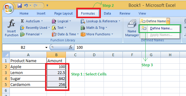
- Give a new Name(PriceTotal in our example) & click Ok. (You can see the range in the bottom refers to section, here absolute referencing is used, $ before the row number/ column letter locks the row/column).

- Now, the next thing is to see that how to use this named range in any of the Excel formulas. For example, if you want to get the sum of all numbers in the above name range then, can say simply write: =SUM(PriceTotal).

Here, B7 =SUM(PriceTotal) = 100 + 22.5 + 843 + 256 (all the numbers in the named range)= 1220.5
Note: The named Range created by this method is restricted to a worksheet.
Method 2: Use the Name Box
Use the following steps to create a named range using the name box :
- Choose the range for which you’d want to give it a name (not the headers).
- Type the name of the range with which you wish to construct the Named Range in the Name Box on the left of the Formula bar.

Note: The Name created this way is available in the entire excel current Workbook.
Method 3: From Selection Option
When you have tabular data and wish to construct named ranges for each column/row, this is the preferred method.
Example: We have 3 columns having headers: Product Name, Amount & Tax Percent.
Use the following steps to create a named range from the selection option :
- Select the complete data set (the 3 columns with the headers).
- Click on the Formulas tab.
- Click Create from Selection (or press Control + Shift + F3).

- After the click, Create Names from Selection’ dialogue box will be opened.

- Check the settings where you have the headers in the Create Names from Selection dialogue box. Because the heading is in the top row, we only select the top row. You can choose both if you have headers in the top row and left column. We only need to check the Left Column option, if the data is organized with the headers only in the left column.
Here we select only Top row because we have headers in the top row.
Result: The data set you selected in column A will be having a named Range: Product_Name (Spaces not allowed, so underscore automatically replaces space)
The data set you selected in column B will be having a named Range: Amount
The data set you selected in column C will be having a named Range: TAX_Percent (Spaces not allowed, so underscore automatically replaces space)
Benefits of Creating Named Ranges in Excel:
The following are benefits of creating & use Named Ranges in Excel :
Instead of using cell references every time, we can directly use Named Reference
Example 1: In the above example, to calculate the sum, we used B7 =SUM(PriceTotal) instead of B7 = SUM(B2:B5) for the above data range.
Example 2: If for the same-named Range, if we write, B9 = SUMIF(PriceTotal,”>50″), then the sum will be equal to the sum of all numbers > 50 in the named range.
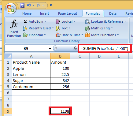
Here, sum is done for all the numbers > 50 in the named range “PriceTotal” = 100+842+256 = 1198.
- To Select Cells, you do not need to return to the data set to choose the cells. You can directly use the Named range, by typing the first few characters of the named range, excel shows a list of named ranges that matches the typed characters.
Example :

As you can see that after just typing Pr, a drop-down list for the available options(formula & named Range) is pooped up.
- The formulas become dynamic using named Ranges:
- Excel formulas become dynamic if we use Named Ranges. In the above example, if we add another cell of Tax Percent (2.5%)& you name it as “TAX” . Now to calculate Final Price (including tax), we can use the Named Range instead of using the value 2.5.
- Now, if later tax is increased to 3%, you just have to update the Named Range, and all the calculations would be done automatically & we will get the Final Price according to the latest tax percent.
- Finding a named cell is less time-consuming.
Using Create From Selection Option :
When generating Named Ranges in Excel, you should be aware of the following naming conventions:
- A letter and underscore character(_), or a backslash, shall be the initial character in a Named Range (). It will display an error if it is anything else is used. Letters, numbers, special characters, a period, or an underscore can make up the remaining characters.
- When establishing named ranges, you can’t use spaces. Tax Percent, for example, cannot be a named range. We can use an underscore, a period, or capital characters if we wish to make a Named Range out of two words, You may, for example, Tax_Percent, TaxPercent, etc.
- In Excel, you can’t use names that are also cell references. You can’t use C1 because it’s also a cell reference.
- You can only have a maximum of 255 characters in a named range.
- For Excel, uppercase and lowercase letters are the same when generating named ranges. For example, if you create a named range called ‘TAX’, you cannot create another named range called ‘Tax’ or ‘tax’.
Name Rows and Columns in Excel:
You may find yourself producing a lot of Named Ranges in Excel when working with large data sets and complex models. It is possible that you can’t recall the name of the Named Range you made. What to do then?
Solutions:
1. Getting the Names of All the Named Ranges
- Click on the formula tab.
- Choose – Use in Formula(In the Defined Named group).

- Choose Paste names & you will get a list of all the Named Ranges in the workbook.

2. Displaying the Matching Named Ranges
As discussed earlier, type a few initial characters, if you have some glimpse about the Name, and a drop-down list of matching ones will be shown.
Editing the Named Range in Excel :
To change/ edit the already created named range, follow these steps :
- Click the Formulas tab.
- Click the name manager(or Ctrl + F3).

- All of the Named Ranges in that workbook will be listed in the Name Manager dialogue box. Double-click the Named Range you’d like to change.

- Edit Name dialog box will pop up, make the modifications.
Example:
Here when we double-click Amount, the edit window for the same get open & we rename that named range from Amount to any other name.

- Click OK and close the name manager window.
Useful Named Range Shortcuts:
When dealing with Named Ranges in Excel, the following keyboard shortcuts can come in use frequently :
- F3: Will give a list of all the Named Ranges and pasting it in any Formula.
- Ctrl + + Shift + F3 : To pop up create Named Ranges from Selection window.
- Ctrl + F3 : To pop up the name manager window directly.
- F1: For Excel Help.
November 15, 2015/
Chris Newman
What Is A Named Range?
Creating a named range allows you to refer to a cell or group of cells with a custom name instead of the usual column/row reference. The HUGE benefit to using Named Ranges is it adds the ability to describe the data inside your cells. Let’s look at a quick example:
Can you tell if shipping costs are charged with the product price?
-
= (B7 + B5 * C4) * (1 + A3)
-
=(ShippingCharge + ProductPrice * Quantity) * (1 + TaxRate)
Hopefully, you can clearly see option number TWO gives you immediate insight to whether the cost of the products includes shipping costs. This allows the user to easily understand how the formula is calculating without having to waste time searching through cells to figure out what is what.
How Do I Use Named Ranges?
As a financial analyst, I play around with a bunch of rates. Examples could be anything from a tax rate to an estimated inflation rate. I use named ranges to organize my variables that either are changed infrequently (ie Month or Year) or something that will be static for a good amount of time (ie inflation rate). Here are a list of common names I use on a regular basis:
-
ReportDate
-
Year
-
Month
-
FcstID
-
TaxRate
-
RawData
Creating Unique Names On The Fly
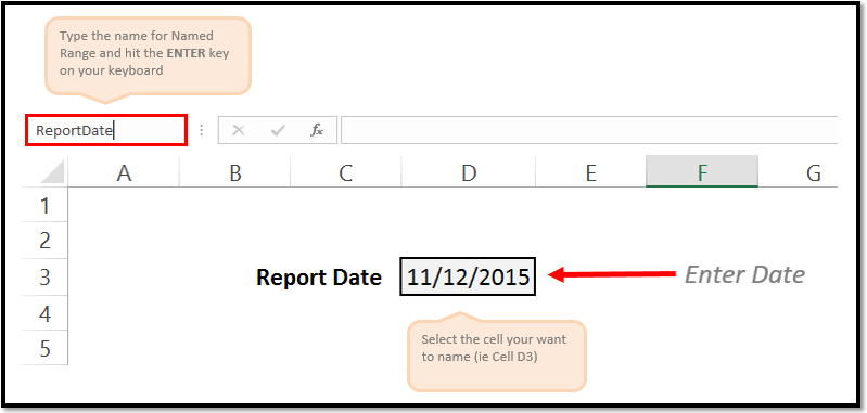
It is super easy to create a Named Range. All you have to do is highlight the cell(s) you want to reference and give it a name in the Name Box. You name cannot have any spaces in it, so if you need to separate words you can either capitalize the beginning of each new word or use an underscore (_). Make sure you hit the ENTER key after you have finished typing the name to confirm the creation of the Named Range.
As a side note, any Named Range created with the Name Box has a Workbook scope. This means the named range can be accessed by any worksheet in your Excel file.
Creating Names With The «Name Manager»
If you want to customize your named ranges even more, you can open up the Name Manager (Formulas tab > Defined Names group > Name Manager button) to edit and create new named ranges.
I won’t go into great detail in this article, but know that with the Name Manager you can
-
Change the name of an existing Named Range
-
Change the reference formula
-
Specify the scope (what worksheets the name can be accessed from)
On To The VBA
Now that you have had a brief overview on Named Ranges, lets dig into some VBA macros you can use to help automate the use of Named Ranges.
Add A Named Range
The below VBA code shows ways you can create various types of named ranges.
Sub NameRange_Add()
‘PURPOSE: Various ways to create a Named Range
‘SOURCE: www.TheSpreadsheetGuru.com
Dim cell As Range
Dim rng As Range
Dim RangeName As String
Dim CellName As String
‘Single Cell Reference (Workbook Scope)
RangeName = «Price»
CellName = «D7»
Set cell = Worksheets(«Sheet1»).Range(CellName)
ThisWorkbook.Names.Add Name:=RangeName, RefersTo:=cell
‘Single Cell Reference (Worksheet Scope)
RangeName = «Year»
CellName = «A2»
Set cell = Worksheets(«Sheet1»).Range(CellName)
Worksheets(«Sheet1»).Names.Add Name:=RangeName, RefersTo:=cell
‘Range of Cells Reference (Workbook Scope)
RangeName = «myData»
CellName = «F9:J18»
Set cell = Worksheets(«Sheet1»).Range(CellName)
ThisWorkbook.Names.Add Name:=RangeName, RefersTo:=cell
‘Secret Named Range (doesn’t show up in Name Manager)
RangeName = «Username»
CellName = «L45»
Set cell = Worksheets(«Sheet1»).Range(CellName)
ThisWorkbook.Names.Add Name:=RangeName, RefersTo:=cell, Visible:=False
End Sub
Loop Through Named Ranges
This VBA macro code shows how you can cycle through the named ranges within your spreadsheet.
Sub NamedRange_Loop()
‘PURPOSE: Delete all Named Ranges in the Active Workbook
‘SOURCE: www.TheSpreadsheetGuru.com
Dim nm As Name
‘Loop through each named range in workbook
For Each nm In ActiveWorkbook.Names
Debug.Print nm.Name, nm.RefersTo
Next nm
‘Loop through each named range scoped to a specific worksheet
For Each nm In Worksheets(«Sheet1»).Names
Debug.Print nm.Name, nm.RefersTo
Next nm
End Sub
Delete All Named Ranges
If you need to clean up a bunch of junk named ranges, this VBA code will let you do it.
Sub NamedRange_DeleteAll()
‘PURPOSE: Delete all Named Ranges in the ActiveWorkbook (Print Areas optional)
‘SOURCE: www.TheSpreadsheetGuru.com
Dim nm As Name
Dim DeleteCount As Long
‘Delete PrintAreas as well?
UserAnswer = MsgBox(«Do you want to skip over Print Areas?», vbYesNoCancel)
If UserAnswer = vbYes Then SkipPrintAreas = True
If UserAnswer = vbCancel Then Exit Sub
‘Error Handler in case Delete Function Errors out
On Error GoTo Skip
‘Loop through each name and delete
For Each nm In ActiveWorkbook.Names
If SkipPrintAreas = True And Right(nm.Name, 10) = «Print_Area» Then GoTo Skip
‘Error Handler in case Delete Function Errors out
On Error GoTo Skip
‘Delete Named Range
nm.Delete
DeleteCount = DeleteCount + 1
Skip:
‘Reset Error Handler
On Error GoTo 0
Next
‘Report Result
If DeleteCount = 1 Then
MsgBox «[1] name was removed from this workbook.»
Else
MsgBox «[» & DeleteCount & «] names were removed from this workbook.»
End If
End Sub
Delete Named Ranges with Error References
This VBA code will delete only Named Ranges with errors in them. These errors can be caused by worksheets being deleted or rows/columns being deleted.
Sub NamedRange_DeleteErrors()
‘PURPOSE: Delete all Named Ranges with #REF error in the ActiveWorkbook
‘SOURCE: www.TheSpreadsheetGuru.com
Dim nm As Name
Dim DeleteCount As Long
‘Loop through each name and delete
For Each nm In ActiveWorkbook.Names
If InStr(1, nm.RefersTo, «#REF!») > 0 Then
‘Error Handler in case Delete Function Errors out
On Error GoTo Skip
‘Delete Named Range
nm.Delete
DeleteCount = DeleteCount + 1
End If
Skip:
‘Reset Error Handler
On Error GoTo 0
Next
‘Report Result
If DeleteCount = 1 Then
MsgBox «[1] errorant name was removed from this workbook.»
Else
MsgBox «[» & DeleteCount & «] errorant names were removed from this workbook.»
End If
End Sub
Anything Missing From This Guide?
Let me know if you have any ideas for other useful VBA macros concerning Named Ranges. Or better yet, share with me your own macros and I can add them to the article for everyone else to see! I look forward to reading your comments below.
About The Author
Hey there! I’m Chris and I run TheSpreadsheetGuru website in my spare time. By day, I’m actually a finance professional who relies on Microsoft Excel quite heavily in the corporate world. I love taking the things I learn in the “real world” and sharing them with everyone here on this site so that you too can become a spreadsheet guru at your company.
Through my years in the corporate world, I’ve been able to pick up on opportunities to make working with Excel better and have built a variety of Excel add-ins, from inserting tickmark symbols to automating copy/pasting from Excel to PowerPoint. If you’d like to keep up to date with the latest Excel news and directly get emailed the most meaningful Excel tips I’ve learned over the years, you can sign up for my free newsletters. I hope I was able to provide you with some value today and I hope to see you back here soon!
— Chris
Founder, TheSpreadsheetGuru.com
Overview on Excel VBA Named Range
In excel we learned how to name a range and use it. Now we will learn how to use this name range in VBA and in addition to that we will also learn how to name a range from VBA. Range is a crucial part of a worksheet as it contains the data for us. Specifically giving names to ranges help us to identify which part of the range contains which data.
Let us begin with how can we name a range in excel and then use it in VBA. In order to name a group of ranges in excel, we simply select the ranges as follows,
Now there is a box where it is mentioned as A1 we click on it and give it a name.
The box is called a name box and we use it to give a name to our range. For the current example, I have given it as a named range. Now once we have given the range name how do we use it in VBA. Suppose we had to change the interior color of the above range previously in VBA what we did in VBA is we referred to the range as follows,
Worksheets(“Sheet1”).Range(“A1:B5”).Interior.Color = Some Color code
Now since we have given the range a name we can now do the following to change the color of the range as follows,
Worksheets(“Sheet1”).Range(“NEW”).Interior.Color = Some Color code
NEW is the range name we have given to cell selection A1:B5. This is how we use name ranges in VBA once we have named them.
Now we can also name the ranges using VBA too well it is a bit lengthy process than above but let us go through it.
To name a range in a worksheet by VBA we use the following code as follows,
Set myWorksheet = ThisWorkbook.Worksheets("Named Range")
Set myNamedRangeWorksheet = myWorksheet.Range("Range Value”)
How to Use Named Range in Excel VBA?
There are two methods to use the Named Range in Excel VBA:
- First is that we name a range in excel and then use it in VBA.
- The second method is we make a named range in VBA itself and use its properties.
Below are the different examples to use the Named Range in Excel:
You can download this VBA Named Range Excel Template here – VBA Named Range Excel Template
Example #1
For the first example let us use the name range we used above by making it in excel worksheet. Follow the below steps:
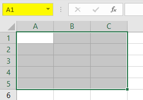
Step 1: Select the range which we want to name first as follows,
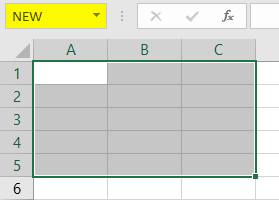
Step 2: There is a name box above the range we use that to give a name to the range, for this example, I have named the ranged as New.
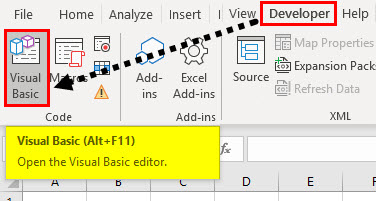
Step 3: Now let us go to VBA, click on Developer’s tab to click on Visual Basic to get into VBA.
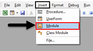
Step 4: Once we are in VBA we need to insert a module so that we can write code in it. Do as follows,
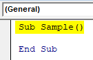
Step 5: Now let us start writing the code, to do that we need to name the macro first as follows,
Code:
Sub Sample()

End Sub
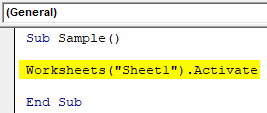
Step 6: Write the following code to activate the worksheet first in order to use the name range.
Code:
Sub Sample()

Worksheets("Sheet1").Activate

End Sub
Step 7: Now let us use our name range as follows,
Code:
Sub Sample()

Worksheets("Sheet1").Activate
Range("NEW").Value = 10

End Sub
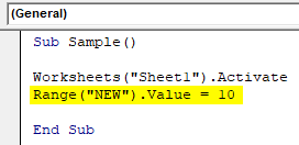
Step 8: Once we run the above code we can see that every cell in our name range has the same value as follows,
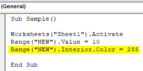
Step 9: Let us also check if we can change the properties of the cell, Let us change the color of the range by using the name range as follows,
Code:
Sub Sample()

Worksheets("Sheet1").Activate
Range("NEW").Value = 10
Range("NEW").Interior.Color = 255

End Sub
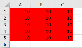
Step 10: Run the above code by pressing F5 or from the run button and see the following result,
Example #2
We will first create a named range by using VBA and the use the properties of the name range in VBA itself. Follow the below steps:
Step 1: Now let us start writing the code, to do that we need to name the macro first as follows,
Code:
Sub Sample1()

End Sub
Step 2: Declare a variable which will store the name of the name range as follows,
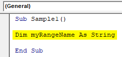
Code:
Sub Sample1()

Dim myRangeName As String

End Sub
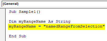
Step 3: Now let us set the name range as follows, in this example whatever we have selected as the range will be our named range,
Code:
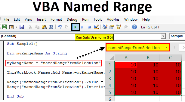
Sub Sample1()

Dim myRangeName As String
myRangeName = "namedRangeFromSelection"

End Sub
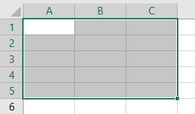
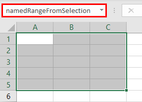
This is what I have in selection for named range cell range A1:C5 in worksheet 2,
Step 4: Now let us name the range by the following code,
Code:
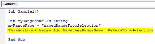
Sub Sample1()

Dim myRangeName As String
myRangeName = "namedRangeFromSelection"
ThisWorkbook.Names.Add Name:=myRangeName, RefersTo:=Selection

End Sub
Step 5: Run the above code we can see that we have created the name range in worksheet 2 by the name of namedrangefromselection,
Step 6: Now let us use this name ranged as we used in the earlier example as follows,
Code:
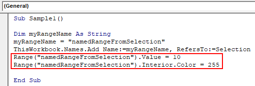
Sub Sample1()

Dim myRangeName As String
myRangeName = "namedRangeFromSelection"
ThisWorkbook.Names.Add Name:=myRangeName, RefersTo:=Selection
Range("namedRangeFromSelection").Value = 10
Range("namedRangeFromSelection").Interior.Color = 255

End Sub
Step 7: Run the above code from the F5 button and see the result as follows,
Things to Remember
- Named Ranges are the name given for a group or range of cells.
- Named range is used to refer to the specific range of cells which needs to be accessed later on.
- We can name a range in both excel or VBA.
- While making a named range in VBA we need to use Add name function in VBA.
Recommended Articles
This is a guide to VBA Named Range. Here we discuss how to use Named Range in Excel VBA along with practical examples and downloadable excel template. You can also go through our other suggested articles –
- Step by Step Guide to VBA Value
- How to Edit Drop Down List in Excel?
- VBA Subscript out of Range
- Import Data into Excel
Named ranges are one of these crusty old features in Excel that few users understand. New users may find them weird and scary, and even old hands may avoid them because they seem pointless and complex.
But named ranges are actually a pretty cool feature. They can make formulas *a lot* easier to create, read, and maintain. And as a bonus, they make formulas easier to reuse (more portable).
In fact, I use named ranges all the time when testing and prototyping formulas. They help me get formulas working faster. I also use named ranges because I’m lazy, and don’t like typing in complex references 
The basics of named ranges in Excel
What is a named range?
A named range is just a human-readable name for a range of cells in Excel. For example, if I name the range A1:A100 «data», I can use MAX to get the maximum value with a simple formula:
=MAX(data) // max value

The beauty of named ranges is that you can use meaningful names in your formulas without thinking about cell references. Once you have a named range, just use it just like a cell reference. All of these formulas are valid with the named range «data»:
=MAX(data) // max value
=MIN(data) // min value
=COUNT(data) // total values
=AVERAGE(data) // min value
Video: How to create a named range
Creating a named range is easy
Creating a named range is fast and easy. Just select a range of cells, and type a name into the name box. When you press return, the name is created:

To quickly test the new range, choose the new name in the dropdown next to the name box. Excel will select the range on the worksheet.
Excel can create names automatically (ctrl + shift + F3)
If you have well structured data with labels, you can have Excel create named ranges for you. Just select the data, along with the labels, and use the «Create from Selection» command on the Formulas tab of the ribbon:

You can also use the keyboard shortcut control + shift + F3.
Using this feature, we can create named ranges for the population of 12 states in one step:

When you click OK, the names are created. You’ll find all newly created names in the drop down menu next to the name box:

With names created, you can use them in formulas like this
=SUM(MN,WI,MI)
Update named ranges in the Name Manager (Control + F3)
Once you create a named range, use the Name Manager (Control + F3) to update as needed. Select the name you want to work with, then change the reference directly (i.e. edit «refers to»), or click the button at right and select a new range.

There’s no need to click the Edit button to update a reference. When you click Close, the range name will be updated.
Note: if you select an entire named range on a worksheet, you can drag to a new location and the reference will be updated automatically. However, I don’t know a way to adjust range references by clicking and dragging directly on the worksheet. If you know a way to do this, chime in below!
See all named ranges (control + F3)
To quickly see all named ranges in a workbook, use the dropdown menu next to the name box.
If you want to see more detail, open the Name Manager (Control + F3), which lists all names with references, and provides a filter as well:

Note: in older versions of Excel on the Mac, there is no Name Manager, and you’ll see the Define Name dialog instead.
Copy and paste all named ranges (F3)
If you want a more persistent record of named ranges in a workbook, you can paste the full list of names anywhere you like. Go to Formulas > Use in Formula (or use the shortcut F3), then choose Paste names > Paste List:

When you click the Paste List button, you’ll see the names and references pasted into the worksheet:

See names directly on the worksheet
If you set the zoom level to less than 40%, Excel will show range names directly on the worksheet:

Thanks for this tip, Felipe!
Names have rules
When creating named ranges, follow these rules:
- Names must begin with a letter, an underscore (_), or a backslash ()
- Names can’t contain spaces and most punctuation characters.
- Names can’t conflict with cell references – you can’t name a range «A1» or «Z100».
- Single letters are OK for names («a», «b», «x», etc.), but the letters «r» and «c» are reserved.
- Names are not case-sensitive – «home», «HOME», and «HoMe» are all the same to Excel.
Named ranges in formulas
Named ranges are easy to use in formulas
For example, lets say you name a cell in your workbook «updated». The idea is you can put the current date in the cell (Ctrl +  and refer to the date elsewhere in the workbook.

The formula in B8 looks like this:
="Updated: "& TEXT(updated, "ddd, mmmm d, yyyy")
You can paste this formula anywhere in the workbook and it will display correctly. Whenever you change the date in «updated», the message will update wherever the formula is used. See this page for more examples.
Named ranges appear when typing a formula
Once you’ve created a named range, it will appear automatically in formulas when you type the first letter of the name. Press the tab key to enter the name when you have a match and want Excel to enter the name.

Named ranges can work like constants
Because named ranges are created in a central location, you can use them like constants without a cell reference. For example, you can create names like «MPG» (miles per gallon) and «CPG» (cost per gallon) with and assign fixed values:

Then you can use these names anywhere you like in formulas, and update their value in one central location.

Named ranges are absolute by default
By default, named ranges behave like absolute references. For example, in this worksheet, the formula to calculate fuel would be:
=C5/$D$2

The reference to D2 is absolute (locked) so the formula can be copied down without D2 changing.
If we name D2 «MPG» the formula becomes:
=C5/MPG

Since MPG is absolute by default, the formula can be copied down column D as-is.
Named ranges can also be relative
Although named ranges are absolute by default, they can also be relative. A relative named range refers to a range that is relative to the position of the active cell at the time the range is created. As a result, relative named ranges are useful building generic formulas that work wherever they are moved.
For example, you can create a generic «CellAbove» named range like this:
- Select cell A2
- Control + F3 to open Name Manager
- Tab into ‘Refers to’ section, then type: =A1
CellAbove will now retrieve the value from the cell above wherever it is it used.
Important: make sure the active cell is at the correct location before creating the name.
Apply named ranges to existing formulas
If you have existing formulas that don’t use named ranges, you can ask Excel to apply the named ranges in the formulas for you. Start by selecting the cells that contain formulas you want to update. Then run Formulas > Define Names > Apply Names.

Excel will then replace references that have a corresponding named range with the name itself.
You can also apply names with find and replace:

Important: Save a backup of your worksheet, and select just the cells you want to change before using find and replace on formulas.
Key benefits of named ranges
Named ranges make formulas easier to read
The biggest single benefit to named ranges is they make formulas easier to read and maintain. This is because they replace cryptic references with meaningful names. For example, consider this worksheet with data on planets in our solar system. Without named ranges, a VLOOKUP formula to fetch «Position» from the table is quite cryptic:
=VLOOKUP($H$4,$B$3:$E$11,2,0)

However, with B3:E11 named «data», and H4 named «planet», we can write formulas like this:
=VLOOKUP(planet,data,2,0) // position
=VLOOKUP(planet,data,3,0) // diameter
=VLOOKUP(planet,data,4,0) // satellites

At a glance, you can see the only difference in these formulas in the column index.
Named ranges make formulas portable and reusable
Named ranges can make it much easier to reuse a formula in a different worksheet. If you define names ahead of time in a worksheet, you can paste in a formula that uses these names and it will «just work». This is a great way to quickly get a formula working.
For example, this formula counts unique values in a range of numeric data:
=SUM(--(FREQUENCY(data,data)>0))
To quickly «port» this formula to your own worksheet, name a range «data» and paste the formula into the worksheet. As long as «data» contains numeric values, the formula will work straightway.
Tip: I recommend that you create the needed range names *first* in the destination workbook, then copy in the formula as text only (i.e. don’t copy the cell that contains the formula in another worksheet, just copy the text of the formula). This stops Excel from creating names on-the-fly and lets you to fully control the name creation process. To copy only formula text, copy text from the formula bar, or copy via another application (i.e. browser, text editor, etc.).
Named ranges can be used for navigation
Named ranges are great for quick navigation. Just select the dropdown menu next to the name box, and choose a name. When you release the mouse, the range will be selected. When a named range exists on another sheet, you’ll be taken to that sheet automatically.

Named ranges work well with hyperlinks
Named ranges make hyperlinks easy. For example, if you name A1 in Sheet1 «home», you can create a hyperlink somewhere else that takes you back there.


To use a named range inside the HYPERLINK function, add a hash (#) in front of the named range:
=HYPERLINK("#home","take me home")
You can use this same syntax to create a hyperlink to a table:
=HYPERLINK("#Table1","Go to Table1")Note: in older versions of Excel you can’t link to a table like this. However, you can define a name equal to a table (i.e. =Table1) and hyperlink to that.
Named ranges for data validation
Names ranges work well for data validation, since they let you use a logically named reference to validate input with a drop down menu. Below, the range G4:G8 is named «statuslist», then apply data validation with a List linked like this:

The result is a dropdown menu in column E that only allows values in the named range:

Dynamic Named Ranges
Names ranges are extremely useful when they automatically adjust to new data in a worksheet. A range set up this way is referred to as a «dynamic named range». There are two ways to make a range dynamic: formulas and tables.
Dynamic named range with a Table
A Table is the easiest way to create a dynamic named range. Select any cell in the data, then use the shortcut Control + T:

When you create an Excel Table, a name is automatically created (e.g. Table1), but you can rename the table as you like. Once you have created a table, it will expand automatically when data is added.

Dynamic named range with a formula
You can also create a dynamic named range with formulas, using functions like OFFSET and INDEX. Although these formulas are moderately complex, they provide a lightweight solution when you don’t want to use a table. The links below provide examples with full explanations:
- Example of dynamic range formula with INDEX
- Example of dynamic range formula with OFFSET
Table names in data validation
Since Excel Tables provide an automatic dynamic range, they would seem to be a natural fit for data validation rules, where the goal is to validate against a list that may be always changing. However, one problem with tables is that you can’t use structured references directly to create data validation or conditional formatting rules. In other words, you can’t use a table name in conditional formatting or data validation input areas.
However, as a workaround, you can define named a named range that points to a table, and then use the named range for data validation or conditional formatting. The video below runs through this approach in detail.
Video: How to use named ranges with tables
Deleting named ranges
Note: If you have formulas that refer to named ranges, you may want to update the formulas first before removing names. Otherwise, you’ll see #NAME? errors in formulas that still refer to deleted names. Always save your worksheet before removing named ranges in case you have problems and need to revert to the original.
Named ranges adjust when deleting and inserting cells
When you delete *part* of a named range, or if insert cells/rows/columns inside a named range, the range reference will adjust accordingly and remain valid. However, if you delete all of the cells that enclose a named range, the named range will lose the reference and display a #REF error. For example, if I name A1 «test», then delete column A, the name manager will show «refers to» as:
=Sheet1!#REF!
Delete names with Name Manager
To remove named ranges from a workbook manually, open the name manager, select a range, and click the Delete button. If you want to remove more than one name at the same time, you can Shift + Click or Ctrl + Click to select multiple names, then delete in one step.
Delete names with errors
If you have a lot of names with reference errors, you can use the filter button in the name manager to filter on names with errors:

Then shift+click to select all names and delete.
Named ranges and Scope
Named ranges in Excel have something called «scope», which determines whether a named range is local to a given worksheet, or global across the entire workbook. Global names have a scope of «workbook», and local names have a scope equal to the sheet name they exist on. For example, the scope for a local name might be «Sheet2».
The purpose of scope
Named ranges with a global scope are useful when you want all sheets in a workbook to have access to certain data, variables, or constants. For example, you might use a global named range a tax rate assumption used in several worksheets.
Local scope
Local scope means a name is works only on the sheet it was created on. This means you can have multiple worksheets in the same workbook that all use the same name. For example, perhaps you have a workbook with monthly tracking sheets (one per month) that use named ranges with the same name, all scoped locally. This might allow you to reuse the same formulas in different sheets. The local scope allows the names in each sheet to work correctly without colliding with names in the other sheets.
To refer to a name with a local scope, you can prefix the sheet name to the range name:
Sheet1!total_revenue
Sheet2!total_revenue
Sheet3!total_revenue
Range names created with the name box automatically have global scope. To override this behavior, add the sheet name when defining the name:
Sheet3!my_new_name
Global scope
Global scope means a name will work anywhere in a workbook. For example, you could name a cell «last_update», enter a date in the cell. Then you can use the formula below to display the date last updated in any worksheet.
=last_update
Global names must be unique within a workbook.
Local scope
Locally scoped named ranges make sense for worksheets that use named ranges for local assumptions only. For example, perhaps you have a workbook with monthly tracking sheets (one per month) that use named ranges with the same name, all scoped locally. The local scope allows the names in each sheet to work correctly without colliding with names in the other sheets.
Managing named range scope
By default, new names created with the namebox are global, and you can’t edit the scope of a named range after it’s created. However, as a workaround, you can delete and recreate a name with the desired scope.
If you want to change several names at once from global to local, sometimes it makes sense to copy the sheet that contains the names. When you duplicate a worksheet that contains named ranges, Excel copies the named ranges to the second sheet, changing the scope to local at the same time. After you have the second sheet with locally scoped names, you can optionally delete the first sheet.
Jan Karel Pieterse and Charles Williams have developed a utility called the Name Manager that provides many useful operations for named ranges. You can download the Name Manager utility here.
Names are one convenient identity. Imagine how we’d be addressed if we didn’t have names? Excel tries to make our lives easier by providing us with a similar convenience.
Excel’s Names feature can be surprisingly powerful for organizing data in Excel. Named Ranges let you name a group of cells and then refer to them as a unit as if they were a single cell.
Using named ranges can make formulas easier to read and understand and provides simple navigation via the Name Box. Named ranges are easy to create and can be used for a variety of purposes.
This tutorial will teach you how to use Names feature in Excel.

What are Named Ranges
In Excel, a cell or a range of cells can be named to make their usage easier. It would be simpler to use a named range directly in a formula or select said range.
You can name:
- a Range of cells,
- a Formula,
- a Constant or
- a Table
Benefits of Creating Named Ranges in Excel
- The prime advantage of named ranges is the ease they provide. You don’t have to keep glancing at certain cells or tables to pick up values or cell references and can use a named range instead.
- Using a named range will save typos that may otherwise occur while typing values or formulas since entering named ranges is a clickable option.
- They are of great help to use in formulas as the named range appears upon typing the first letter of the name.
- Named ranges make formulas movable and they can be used from sheet to sheet and workbook to workbook.
- A dynamic named range can automatically account for expanding and contracting data (when values are added or deleted from a dataset) without having to change the formula or recalculate.
- A named range can be used for data validation (creating drop-down menus) without much hassle.
- Hyperlinks can quickly be created from existing named ranges.
- Named ranges make navigation and directing very easy. You can click on a named range in the Name Box and arrive at the named range.
- For all the above benefits that named ranges deliver, they are very simple and quick to create.
Rules for naming Named Ranges
There are several pointers not to trespass while creating named ranges:
- A name should have less than 255 characters.
- A name should not have space and punctuation characters (exceptions mentioned as follows).
- A name’s first character has to be a letter, an underscore ( _ ), or a backslash ( ).
- A name may contain a question mark but never as a first character.
- A name is not case-sensitive. (sale, Sale, and SALE are treated as one name).
- A name must not resemble a cell reference (e.g., A1, A$1).
- A name may be a single letter name but must not be r, R, c, or C as «R» and «C» signify row and column selection shortcuts.
How to Create Named Ranges in Excel
There are two methods to create named ranges in excel. We will see both these methods in this section.
Let’s say we have the data as shown below and we want to create two named ranges – one for the History marks and the second one for the Geography marks.

We will create these two named ranges using two different methods to help you get a hang of both methods.
Method 1 – Creating Named Ranges from the Name Box
The how-to here is pretty simple. Select the range, enter the desired name in the «name box» and press Enter. Done! Really! We can show you how easy this is with a visual.
Here’s how it’s done:
- For naming the History marks range, we will select the History marks i.e., range C3:C7.

- Click on the name box.
- Enter the desired name («History» in this case).

- Press the Enter key.
Method 2 – Creating Named Ranges from the ‘Define Name’ Option
Names can also be created from the «Define Name» button, in the formulas tab. To use this method follow the below steps:
- Select the range which you want to name, in our case it will be D3:D7.
- Navigate to the «Formulas Tab» and click the «Define Name» button.

- Now, in the «New Name» window enter the desired name for the named range.

- After entering the desired name click the «OK» button and it is done.
How to Edit Named Ranges in Excel
Suppose you accidentally missed a cell in the range or want to change the name of your named range. This means the named range needs to be edited.
Named ranges can be managed through the «Name Manager» which can be found under the «Formulas» tab > Name Manager or can be accessed through the keyboard shortcut Ctrl + F3.

This is what you will see when you open the Name Manager:

Here, you can see the named ranges in your sheet and their details. Double click the named range you wish to edit or select the named range and click the «Edit…» button.

Clicking on the «Edit…» button will open the «Edit Name» window where you can edit the name or the cell range of the named range. When done, click «OK» and then click the «Close» button on the Name Manager.
How to Delete Named Ranges
The Name Manager can also be used to delete named ranges. Click the named range you wish to remove, press the «Delete» button.

You will get a pop-up confirmation asking whether you want to delete the named range or not. Press «OK» and that will delete your chosen named range.

Note that the Name Manager also has a «Filter» button that can be used for filtering the names and only viewing the relevant names at a given time. It can be quite handy when you have a lot of names to deal with.
Recommended Reading: How to Lock and Protect Cells in Excel
How to Create Names from Cell Text
For batch information where the data is in the columnar or row format (i.e., in either columnar form with headings at the top and its relevant data below. Or in rows with headings on the left and its data on the right) there is a quicker way of naming ranges. We can use the «Create from Selection» feature in Excel to give the heading’s name to the range. Here is how:
So, we have the dataset containing marks scored by students in various subjects. The layout is in columnar form. We can use the «Create from Selection» feature in this case as –

- Select the range and the heading. We will select columns C, D, E, and F to name each range according to its heading.

- In the «Formulas» tab, click «Create from Selection» or use the keyboard shortcut Ctrl + Shift + F3. This is what you should see:

- According to the layout of your dataset, select the row or column where the headings need to be picked from. For our case, we will select the «Top row» option as headings. «Marks in History», «Marks in Geography», «Marks in Science», and «Marks in Math» are in the top row.
- After selecting the appropriate options click «OK».
Doing this has created multiple named ranges for our data. You can see from the drop-down in the Name Box that we have 4 named ranges created according to the headings of each column.

Note that the spaces in headings are replaced with underscores while creating the names.
Named Ranges with Hyperlinks
If you thought named ranges made you bounce around with ease through worksheets, wait for their synergy with hyperlinks. Named ranges make hyperlinking a smoother process as data required for hyperlinking would already be grouped and named. Let’s show you how this will work.
For the sake of this example let’s assume that we have another named range «Student» in Sheet2 as shown.

We will hyperlink the Student column from Sheet1 to direct us to the student range in Sheet2.
- Select the Student range in Sheet2 (i.e., B3:B7).

- Right-click the selected area and click on «Link». The «Insert Hyperlink» window is what you should see.

- We will select «Student» from «Defined Names» which we have already defined in Sheet2.
- Click «OK».

We have hyperlinked the Student Names to Sheet2 using the «Student» named range. Clicking on any of the marks should take us to the «Student» range on Sheet2. Let’s check.

Affirmative!
How to Create an Excel Name for a Constant
The Name Manager can also be used to create a name for a constant value. This constant value will not be a cell reference on the sheet but it can be used by its name in formulas.
For our example, we will use a named constant to calculate the percentage of the overall marks of each of 5 students. We start by accessing the Name Manager and applying for a new name.

The percentage will be calculated by dividing the sum of the attained marks by the total (each subject is marked out of 50. Which makes 50 x 4 = 200). We will set «200» as our named constant and give it the name «total».
Using «total», we can calculate the percentages without having to refer to «200».

Here, we have substituted «200» for «total» and calculated each student’s overall percentage.
How to Make a Named Formula
Taking the above example, what if we named the whole formula and get the same results? Sounds like a good bargain for smart input. Let’s see how to do that.
We first head to good old Name Manager and «New Name» again. We will name our formula «Percentage». The reference of this name is shown as
=SUM(Sheet2!$C3:$F3)/total

The range of the SUM in the formula is «C3:F3». The columns have been locked into absolute references by the $ sign. Notice that the rows have not been locked as absolute references so that the formula can be dragged to apply to all the rows.

Now just by using «Percentage», we can use the named formula to calculate the students’ percentages.
Named Ranges for Data Validation
Named ranges make the «Data Validation» feature in Excel a breeze. You can create a drop-down menu with values from a named range.
This comes with some advantages. You can simply refer to the named range in the Data Validation window instead of having to directly enter the cell ranges. It also gives a point of relevance to see the named range in sight. Let’s see how it’s done.
Let’s assume – we have a list of products and their prices and discounts. Our objective here is to calculate the discounted price for each product after entering its relevant discount. Instead of copy-pasting each discount, we want the option to select the discount from a drop-down menu for each cell in column D.

We will create a drop-down menu with the «Discount» named range (G3:G6).
- Select the cells for which you want to create the drop-downs (D3:D9 for our case).

- Under the «Data» tab, in the «Data Tools» section, select «Data Validation» dropdown and click the next «Data Validation» option.
- Inside the «Data Validation» window, under «Allow», choose «List» and enter the required named range under «Source». We will enter the reference of our «Discount» range here.

- Click «OK». This has very conveniently created drop-down menus for all cells D3:D9, taking values from the «Discount» named range.

- Now we can select the respective discounts and arrive at our «Price after discount».
See all Names Directly on the Worksheet
There is a small hack that allows you to see all the names directly on the worksheet. You can view all your named ranges (marked with the names) on the sheet if you zoom out to anything less than 40%. We’ll follow that religiously and zoom out at 39%.

The only thing amiss about this is that the named range text is like a watermark; it’s not opaque and will not work so well for small and narrow columns. This hack is suitable for data with a wide-set column or several more rows so the name of the range can be seen. Otherwise, it would be on the brink of being unnoticeable.
Scope of a Name
If you open the Name Manager and have a look at the named ranges, you will find that each named range has a scope (e.g., Sheet1, Sheet2, Workbook, etc.) against it.

Scope refers to the location, or level, within which the name is recognized. For instance, in the above image «range4» can only be used within Sheet1 whereas all the other names can be used across the entire workbook.
Based on this there can be 2 levels of scopes:
- Local worksheet scope
- Global workbook scope
Local Worksheet Scope
Locally scoped names can only be recognized and used on the sheet it is created upon. This implies that inside a single workbook we can have the same locally scoped names (each within a separate worksheet). For instance – you can have a yearly expense workbook with a worksheet for each month and then we can have a single locally scoped name within each worksheet.
Pro Tip: Named ranges made using the Name Box have global scope by default. However, you can tie the named range down to a sheet (in other words, make it locally scoped) simply by using the sheet’s name before the range’s name (with an exclamation mark).
Sheet1!Expenses
Global Workbook scope
Globally scoped names can be recognized and used across the whole workbook. Global names must always be unique within the workbook. For instance – we can create a global name to define the value of a constant like pi (as 3.14) and use it across the whole workbook.
Creating Dynamic Named Ranges in Excel
Up until now with all the examples above, we can say that if we were to expand on the data by adding more values, the formulas already applied wouldn’t account for the new values. This means that whenever values will be added to the dataset of the named range (e.g., B2:B15) which expands the dataset to B2:B20, the named range will still not account for the additional 5 values and remain a named range for B2:B15. This means the named range is static as opposed to a dynamic named range. The additional step that would need to be taken to fix this is to edit the named range and modify the range mentioned.
A dynamic named range on the contrary will itself adjust for changes in the range. To make our named range dynamic, we will add a function to the reference of the named range. If this sounds too complicated, let us show you how it’s done.
There are a couple of ways of creating a dynamic named range. One of them is using the OFFSET function. The drawback is however that OFFSET is a volatile function; with each and every change in a worksheet, OFFSET recalculates. This is not an issue for an uncomplicated worksheet with small datasets. But with complex and large worksheets, you will find that OFFSET slows things down. In such a case, the other way to create a dynamic named range is using the INDEX function.
So if you can use OFFSET for small datasets and INDEX for large ones, why not just master the INDEX function and use that? So this use of the INDEX function for dynamic named ranges is what we’ll be tapping into right now. Let’s see an example:

Taking simple sales data, we will add a dynamic named range that we will later use to calculate the total sales:
- Open the «Name Manager» > click the «New Name» option.
- Set the desired name (we are naming our named range «Sales»).

- In «Refers to», feed the following formula, and click «OK».
=$C$3:INDEX($C$3:$C$1048576,COUNTIF($C$3:$C$1048576,"<>"&" "))

We have used the SUM function to total the named range «Sales». It has given us a total of «3186» which is also confirmed from selecting the cells with the results displayed in the status bar below.
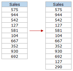
Now let’s add some values to this dataset to see if the formula applied complies with changes in the data.

We have added new sales data and the named range has updated itself because of the formula we have put in to build the range. So how does this formula work?
Let’s see the formula again:
=$C$3:INDEX($C$3:$C$1048576,COUNTIF($C$3:$C$1048576,"<>"&" "))
Since we’re using the INDEX function in the formula, let’s get familiar with it. The INDEX function returns a value or cell reference of a particular cell in a given range. The part we need to work with right now is the return of a cell reference.
The COUNTIF function counts the number of cells within a range that meets the given condition. The range given to COUNTIF is C3:C1048576. COUNTIF needs to look through the entire C column ahead of C3 (if you press Ctrl + down key, you will find the last row given in Excel which is row number 1048576. That is why we have used C1048576 in our formula. According to how big or small your data is, you can refer to any row ahead of your last value, suppose 100 rows ahead of your last value. In this way the formula will account for all changes made up to the last-mentioned row).
The condition given to COUNTIF is counting the number of cells from C3 to C1048576 that should not be equal to (defined by «<>») blank cells (defined by » «). Take note that this will work only if the data does not consist of blank cells as the blank cells are the ones to be ignored by the function.
According to this condition, the non-blank cells that COUNTIF was able to find from the given range were C3:C9. Passing this result to the INDEX function, INDEX then returns the value of the last item of the list (which would be C9’s value i.e., 404). The formula starts with the first cell that we need to include in our named range (i.e. C3, fed as an absolute reference by «$» signs). Using this reference before the INDEX function makes INDEX return the cell reference instead of the value which will then be C9.
The result of the whole formula has worked like this:

Note: Dynamic named ranges aren’t shown in the Name Box. Use the Name Manager to see all named ranges (static and dynamic).
Named Range Shortcuts
The more matters are sitting on your fingertips, the better. To wrap things up, here are some useful keyboard shortcuts with named ranges that should move you around the sheet even faster.
- F3 – Pops up a «Paste Name» dialogue box for pasting a named range from the full list of named ranges.
- Ctrl + F3 – Opens «Name Manager»
- Ctrl + alt + F3 – Pops up «New Name» dialog box for creating a new named range.
- Ctrl + shift + F3 – Pops up «Create Names from Selection» dialog box for creating named ranges from headings/titles.
- F5 – Pops up the «Go To» dialog box for navigating to the chosen named range from the full list of named ranges.
With that, we’ve discussed the ins and outs of the Named Ranges in Excel. They are simple, but extremely useful while working with larger datasets and multiple ranges. While you solidify your expertise with some practice, we’ll have another awesome tutorial ready for you ready!