
Excel for Microsoft 365 Excel for Microsoft 365 for Mac Excel 2021 Excel 2021 for Mac Excel 2019 Excel 2019 for Mac Excel 2016 Excel 2016 for Mac Excel 2013 Excel 2010 More…Less
Scatter charts and line charts look very similar, especially when a scatter chart is displayed with connecting lines. However, the way each of these chart types plots data along the horizontal axis (also known as the x-axis) and the vertical axis (also known as the y-axis) is very different.
Before you choose either of these chart types, you might want to learn more about the differences and find out when it’s better to use a scatter chart instead of a line chart, or the other way around.
The main difference between scatter and line charts is the way they plot data on the horizontal axis. For example, when you use the following worksheet data to create a scatter chart and a line chart, you can see that the data is distributed differently.
In a scatter chart, the daily rainfall values from column A are displayed as x values on the horizontal (x) axis, and the particulate values from column B are displayed as values on the vertical (y) axis. Often referred to as an xy chart, a scatter chart never displays categories on the horizontal axis.
A scatter chart always has two value axes to show one set of numerical data along a horizontal (value) axis and another set of numerical values along a vertical (value) axis. The chart displays points at the intersection of an x and y numerical value, combining these values into single data points. These data points may be distributed evenly or unevenly across the horizontal axis, depending on the data.
The first data point to appear in the scatter chart represents both a y value of 137 (particulate) and an x value of 1.9 (daily rainfall). These numbers represent the values in cell A9 and B9 on the worksheet.
In a line chart, however, the same daily rainfall and particulate values are displayed as two separate data points, which are evenly distributed along the horizontal axis. This is because a line chart only has one value axis (the vertical axis). The horizontal axis of a line chart only shows evenly spaced groupings (categories) of data. Because categories were not provided in the data, they were automatically generated, for example, 1, 2, 3, and so on.
This is a good example of when not to use a line chart.
A line chart distributes category data evenly along a horizontal (category) axis , and distributes all numerical value data along a vertical (value) axis.
The particulate y value of 137 (cell B9) and the daily rainfall x value of 1.9 (cell A9) are displayed as separate data points in the line chart. Neither of these data points is the first data point displayed in the chart — instead, the first data point for each data series refers to the values in the first data row on the worksheet (cell A2 and B2).
Axis type and scaling differences
Because the horizontal axis of a scatter chart is always a value axis, it can display numeric values or date values (such as days or hours) that are represented as numerical values. To display the numeric values along the horizontal axis with greater flexibility, you can change the scaling options on this axis the same way that you can change the scaling options of a vertical axis.
Because the horizontal axis of a line chart is a category axis, it can be only a text axis or a date axis. A text axis displays text only (non-numerical data or numerical categories that are not values) at evenly spaced intervals. A date axis displays dates in chronological order at specific intervals or base units, such as the number of days, months, or years, even if the dates on the worksheet are not in order or in the same base units.
The scaling options of a category axis are limited compared with the scaling options of a value axis. The available scaling options also depend on the type of axis that you use.
Scatter charts are commonly used for displaying and comparing numeric values, such as scientific, statistical, and engineering data. These charts are useful to show the relationships among the numeric values in several data series, and they can plot two groups of numbers as one series of xy coordinates.
Line charts can display continuous data over time, set against a common scale, and are therefore ideal for showing trends in data at equal intervals or over time. In a line chart, category data is distributed evenly along the horizontal axis, and all value data is distributed evenly along the vertical axis. As a general rule, use a line chart if your data has non-numeric x values — for numeric x values, it is usually better to use a scatter chart.
Consider using a scatter chart instead of a line chart if you want to:
-
Change the scale of the horizontal axis Because the horizontal axis of a scatter chart is a value axis, more scaling options are available.
-
Use a logarithmic scale on the horizontal axis You can turn the horizontal axis into a logarithmic scale.
-
Display worksheet data that includes pairs or grouped sets of values In a scatter chart, you can adjust the independent scales of the axes to reveal more information about the grouped values.
-
Show patterns in large sets of data Scatter charts are useful for illustrating the patterns in the data, for example by showing linear or non-linear trends, clusters, and outliers.
-
Compare large numbers of data points without regard to time The more data that you include in a scatter chart, the better the comparisons that you can make.
Consider using a line chart instead of a scatter chart if you want to:
-
Use text labels along the horizontal axis These text labels can represent evenly spaced values such as months, quarters, or fiscal years.
-
Use a small number of numerical labels along the horizontal axis If you use a few, evenly spaced numerical labels that represent a time interval, such as years, you can use a line chart.
-
Use a time scale along the horizontal axis If you want to display dates in chronological order at specific intervals or base units, such as the number of days, months, or years, even if the dates on the worksheet are not in order or in the same base units, use a line chart.
Note: The following procedure applies to Office 2013 and newer versions. Office 2010 steps?
Create a scatter chart
So, how did we create this scatter chart? The following procedure will help you create a scatter chart with similar results. For this chart, we used the example worksheet data. You can copy this data to your worksheet, or you can use your own data.
-
Copy the example worksheet data into a blank worksheet, or open the worksheet that contains the data you want to plot in a scatter chart.
1
2
3
4
5
6
7
8
9
10
11
A
B
Daily Rainfall
Particulate
4.1
122
4.3
117
5.7
112
5.4
114
5.9
110
5.0
114
3.6
128
1.9
137
7.3
104
-
Select the data you want to plot in the scatter chart.
-
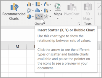
Click the Insert tab, and then click Insert Scatter (X, Y) or Bubble Chart.

-
Click Scatter.
Tip: You can rest the mouse on any chart type to see its name.
-
Click the chart area of the chart to display the Design and Format tabs.
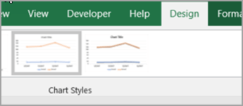
-
Click the Design tab, and then click the chart style you want to use.
-
Click the chart title and type the text you want.
-
To change the font size of the chart title, right-click the title, click Font, and then enter the size that you want in the Size box. Click OK.
-
Click the chart area of the chart.
-
On the Design tab, click Add Chart Element > Axis Titles, and then do the following:
-
To add a horizontal axis title, click Primary Horizontal.
-
To add a vertical axis title, click Primary Vertical.
-
Click each title, type the text that you want, and then press Enter.
-
For more title formatting options, on the Format tab, in the Chart Elements box, select the title from the list, and then click Format Selection. A Format Title pane will appear. Click Size & Properties
, and then you can choose Vertical alignment, Text direction, or Custom angle.
-
-
Click the plot area of the chart, or on the Format tab, in the Chart Elements box, select Plot Area from the list of chart elements.
-
On the Format tab, in the Shape Styles group, click the More button
, and then click the effect that you want to use. -
Click the chart area of the chart, or on the Format tab, in the Chart Elements box, select Chart Area from the list of chart elements.
-
On the Format tab, in the Shape Styles group, click the More button
, and then click the effect that you want to use. -
If you want to use theme colors that are different from the default theme that is applied to your workbook, do the following:
-
On the Page Layout tab, in the Themes group, click Themes.
-
Under Office, click the theme that you want to use.
-
 , and then you can choose Vertical alignment, Text direction, or Custom angle.
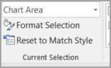
 , and then click the effect that you want to use.
Create a line chart

So, how did we create this line chart? The following procedure will help you create a line chart with similar results. For this chart, we used the example worksheet data. You can copy this data to your worksheet, or you can use your own data.
-
Copy the example worksheet data into a blank worksheet, or open the worksheet that contains the data that you want to plot into a line chart.
1
2
3
4
5
6
7
8
9
10
11
A
B
C
Date
Daily Rainfall
Particulate
1/1/07
4.1
122
1/2/07
4.3
117
1/3/07
5.7
112
1/4/07
5.4
114
1/5/07
5.9
110
1/6/07
5.0
114
1/7/07
3.6
128
1/8/07
1.9
137
1/9/07
7.3
104
-
Select the data that you want to plot in the line chart.
-
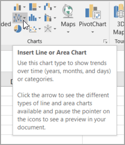
Click the Insert tab, and then click Insert Line or Area Chart.
-
Click Line with Markers.
-
Click the chart area of the chart to display the Design and Format tabs.
-
Click the Design tab, and then click the chart style you want to use.
-
Click the chart title and type the text you want.
-
To change the font size of the chart title, right-click the title, click Font, and then enter the size that you want in the Size box. Click OK.
-
Click the chart area of the chart.
-
On the chart, click the legend, or add it from a list of chart elements (on the Design tab, click Add Chart Element > Legend, and then select a location for the legend).
-
To plot one of the data series along a secondary vertical axis, click the data series, or select it from a list of chart elements (on the Format tab, in the Current Selection group, click Chart Elements).
-
On the Format tab, in the Current Selection group, click Format Selection. The Format Data Series task pane appears.
-
Under Series Options, select Secondary Axis, and then click Close.
-
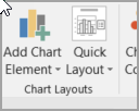
On the Design tab, in the Chart Layouts group, click Add Chart Element, and then do the following:
-
To add a primary vertical axis title, click Axis Title >Primary Vertical. and then on the Format Axis Title pane, click Size & Properties
to configure the type of vertical axis title that you want. -
To add a secondary vertical axis title, click Axis Title > Secondary Vertical, and then on the Format Axis Title pane, click Size & Properties
to configure the type of vertical axis title that you want. -
Click each title, type the text that you want, and then press Enter
-
-
Click the plot area of the chart, or select it from a list of chart elements (Format tab, Current Selection group, Chart Elements box).
-
On the Format tab, in the Shape Styles group, click the More button
, and then click the effect that you want to use.
-
Click the chart area of the chart.
-
On the Format tab, in the Shape Styles group, click the More button
, and then click the effect that you want to use. -
If you want to use theme colors that are different from the default theme that is applied to your workbook, do the following:
-
On the Page Layout tab, in the Themes group, click Themes.
-
Under Office, click the theme that you want to use.
-
Create a scatter or line chart in Office 2010
So, how did we create this scatter chart? The following procedure will help you create a scatter chart with similar results. For this chart, we used the example worksheet data. You can copy this data to your worksheet, or you can use your own data.
-
Copy the example worksheet data into a blank worksheet, or open the worksheet that contains the data that you want to plot into a scatter chart.
1
2
3
4
5
6
7
8
9
10
11
A
B
Daily Rainfall
Particulate
4.1
122
4.3
117
5.7
112
5.4
114
5.9
110
5.0
114
3.6
128
1.9
137
7.3
104
-
Select the data that you want to plot in the scatter chart.
-
On the Insert tab, in the Charts group, click Scatter.
-
Click Scatter with only Markers.
Tip: You can rest the mouse on any chart type to see its name.
-
Click the chart area of the chart.
This displays the Chart Tools, adding the Design, Layout, and Format tabs.
-
On the Design tab, in the Chart Styles group, click the chart style that you want to use.
For our scatter chart, we used Style 26.
-
On the Layout tab, click Chart Title and then select a location for the title from the drop-down list.
We chose Above Chart.
-
Click the chart title, and then type the text that you want.
For our scatter chart, we typed Particulate Levels in Rainfall.
-
To reduce the size of the chart title, right-click the title, and then enter the size that you want in the Font Size box on the shortcut menu.
For our scatter chart, we used 14.
-
Click the chart area of the chart.
-
On the Layout tab, in the Labels group, click Axis Titles, and then do the following:
-
To add a horizontal axis title, click Primary Horizontal Axis Title, and then click Title Below Axis.
-
To add a vertical axis title, click Primary Vertical Axis Title, and then click the type of vertical axis title that you want.
For our scatter chart, we used Rotated Title.
-
Click each title, type the text that you want, and then press Enter.
For our scatter chart, we typed Daily Rainfall in the horizontal axis title, and Particulate level in the vertical axis title.
-
-
Click the plot area of the chart, or select Plot Area from a list of chart elements (Layout tab, Current Selection group, Chart Elements box).
-
On the Format tab, in the Shape Styles group, click the More button
, and then click the effect that you want to use.For our scatter chart, we used the Subtle Effect — Accent 3.
-
Click the chart area of the chart.
-
On the Format tab, in the Shape Styles group, click the More button
, and then click the effect that you want to use.For our scatter chart, we used the Subtle Effect — Accent 1.
-
If you want to use theme colors that are different from the default theme that is applied to your workbook, do the following:
-
On the Page Layout tab, in the Themes group, click Themes.
-
Under Built-in, click the theme that you want to use.
For our line chart, we used the Office theme.
-
So, how did we create this line chart? The following procedure will help you create a line chart with similar results. For this chart, we used the example worksheet data. You can copy this data to your worksheet, or you can use your own data.
-
Copy the example worksheet data into a blank worksheet, or open the worksheet that contains the data that you want to plot into a line chart.
1
2
3
4
5
6
7
8
9
10
11
A
B
C
Date
Daily Rainfall
Particulate
1/1/07
4.1
122
1/2/07
4.3
117
1/3/07
5.7
112
1/4/07
5.4
114
1/5/07
5.9
110
1/6/07
5.0
114
1/7/07
3.6
128
1/8/07
1.9
137
1/9/07
7.3
104
-
Select the data that you want to plot in the line chart.
-
On the Insert tab, in the Charts group, click Line.
-
Click Line with Markers.
-
Click the chart area of the chart.
This displays the Chart Tools, adding the Design, Layout, and Format tabs.
-
On the Design tab, in the Chart Styles group, click the chart style that you want to use.
For our line chart, we used Style 2.
-
On the Layout tab, in the Labels group, click Chart Title, and then click Above Chart.
-
Click the chart title, and then type the text that you want.
For our line chart, we typed Particulate Levels in Rainfall.
-
To reduce the size of the chart title, right-click the title, and then enter the size that you want in the Size box on the shortcut menu.
For our line chart, we used 14.
-
On the chart, click the legend, or select it from a list of chart elements (Layout tab, Current Selection group, Chart Elements box).
-
On the Layout tab, in the Labels group, click Legend, and then click the position that you want.
For our line chart, we used Show Legend at Top.
-
To plot one of the data series along a secondary vertical axis, click the data series for Rainfall, or select it from a list of chart elements (Layout tab, Current Selection group, Chart Elements box).
-
On the Layout tab, in the Current Selection group, click Format Selection.
-
Under Series Options, select Secondary Axis, and then click Close.
-
On the Layout tab, in the Labels group, click Axis Titles, and then do the following:
-
To add a primary vertical axis title, click Primary Vertical Axis Title, and then click the type of vertical axis title that you want.
For our line chart, we used Rotated Title.
-
To add a secondary vertical axis title, click Secondary Vertical Axis Title, and then click the type of vertical axis title that you want.
For our line chart, we used Rotated Title.
-
Click each title, type the text that you want, and then press ENTER.
For our line chart, we typed Particulate level in the primary vertical axis title, and Daily Rainfall in the secondary vertical axis title.
-
-
Click the plot area of the chart, or select it from a list of chart elements (Layout tab, Current Selection group, Chart Elements box).
-
On the Format tab, in the Shape Styles group, click the More button
, and then click the effect that you want to use.For our line chart, we used the Subtle Effect — Dark 1.
-
Click the chart area of the chart.
-
On the Format tab, in the Shape Styles group, click the More button
, and then click the effect that you want to use.For our line chart, we used the Subtle Effect — Accent 3.
-
If you want to use theme colors that are different from the default theme that is applied to your workbook, do the following:
-
On the Page Layout tab, in the Themes group, click Themes.
-
Under Built-in, click the theme that you want to use.
For our line chart, we used the Office theme.
-
Create a scatter chart
-
Select the data you want to plot in the chart.
-
Click the Insert tab, and then click X Y Scatter, and under Scatter, pick a chart.
-
With the chart selected, click the Chart Design tab to do any of the following:
-
Click Add Chart Element to modify details like the title, labels, and the legend.
-
Click Quick Layout to choose from predefined sets of chart elements.
-
Click one of the previews in the style gallery to change the layout or style.
-
Click Switch Row/Column or Select Data to change the data view.
-
-
With the chart selected, click the Design tab to optionally change the shape fill, outline, or effects of chart elements.
Create a line chart
-
Select the data you want to plot in the chart.
-
Click the Insert tab, and then click Line, and pick an option from the available line chart styles .
-
With the chart selected, click the Chart Design tab to do any of the following:
-
Click Add Chart Element to modify details like the title, labels, and the legend.
-
Click Quick Layout to choose from predefined sets of chart elements.
-
Click one of the previews in the style gallery to change the layout or style.
-
Click Switch Row/Column or Select Data to change the data view.
-
-
With the chart selected, click the Design tab to optionally change the shape fill, outline, or effects of chart elements.
See Also
Save a custom chart as a template
Need more help?
Want more options?
Explore subscription benefits, browse training courses, learn how to secure your device, and more.
Communities help you ask and answer questions, give feedback, and hear from experts with rich knowledge.

Plots in Excel (Table of Contents)
- Introduction to Plots in Excel
- Examples of Plots in Excel
Introduction to Plots in Excel
Plots are charts andn graphs which are used to visualize and interpret data so that values for two different variables can be represented along the two axes (horizontal axis, i.e. the x axis and vertical axis, i.e. the y axis). Plots are basically scatter charts generally used to show a graphical relationship between two variables
Scatter plots use the Cartesian axes or coordinates so as to display the two data sets’ values.
In MS Excel, some layouts that are available for scatter plot are:
- Simple Scatter plot.
- Scatter with smooth lines and markers.
- Scatter with smooth lines.
- Scatter with straight lines and markers.
- Scatter with straight lines.
- Bubble chart.
- 3-D Bubble chart.
We can interpret the scatter plots in the following manner:
- If the data points on the plot look like they are randomly scattered, then it implies that there is no correlation between the two variables.
- If the data points on a plot are spread widely on the plane, then it implies that the correlation between two variables is weak.
- The correlation between two variables is said to be strong if the data points are concentrated around a line on the plot.
- The correlation between two datasets is positive If the data points’ pattern on the plot goes from lower left to upper right
- The correlation between two datasets is negative if the data points’ pattern on the plot goes from upper left to lower right,
Examples of Plots in Excel
Lets us discuss the examples of Plots in Excel.
You can download this Plots Excel Template here – Plots Excel Template
Example #1 – Simple Scatter Plot
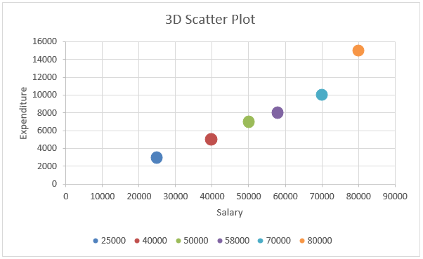
Let us suppose there is an interrelated dataset where we have some people’s monthly salaries and their expenditures. Now the relation between salary and expenditure can be plotted in Excel with the help of a scatter plot.
We have the following data of monthly salaries and expenditures in an Excel file:

Now in order to create a scatter plot for this data in Excel, the following steps can be used:
- Select the dataset and click on the ‘Insert’ tab. Now select ‘Scatter Chart’:

- With this, we will have the data plotted as follows:


Now the chart title can be changed by double-clicking on it and then renaming it:

- Now right click on the scatter lot -> Click on ‘Select Data’:

- On doing this, we will get a popup window:

- In the resulting window, select ‘Salary’ in the section: ‘Legend Entries’, and then select‘Remove’.

- Now in the section ‘Legend Entries’, select ‘Expenditure’ in this window, and choose ‘Edit’ :

- With this, we will have a popup window for the edit series:

- Now in this ‘Edit Series’ window, select ‘Salary’ range under ‘Series X values’:

- This will finally generate the below scatter plot:

- Now right-click on any data point or dot) -> Select ‘Format data Series’:

- With this, we will have a ‘Format Series’ dialog box. In this, click on ‘Effects’ and choose ‘3-D Format’:


- Now under ‘3-D Format’, select ‘circle’ type top level:

- Now in the ‘Format Series’, choose ‘Fill & Line’ and select ‘Marker’:

- Expand the ‘Fill’ option in the ‘Marker’ section -> Select ‘Vary colors by point’:
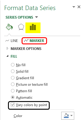
With this, each dot or data point will be represented with a different colour
- Now expand ‘Marker Options’ in the ‘Marker’ section. Choose ‘Built-in’ and then increase the value of size:
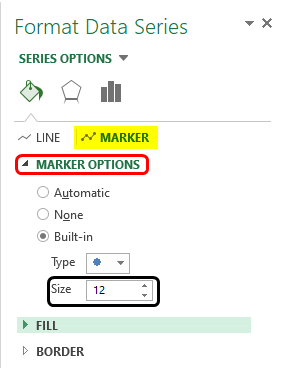
With this, the data points’ size will be increased.
- Now on the right of the plot, click on the ‘Plus’ icon in order to open the ‘Chart Elements’ dialog box:
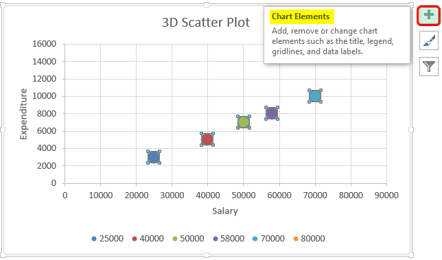
- Now check mark ‘Axis Titles’in the ‘Chart Elements’ dialog box. On doing this,we will have an ‘Axis Title’ textbox on both the axes. (horizontal and vertical
<img class=”alignnone size-full wp-image-343071″ src=”https://www.educba.com/academy/wp-content/uploads/2020/04/Axis-Title.png” alt=%2
Содержание
- How to Graph an Equation / Function – Excel & Google Sheets
- How to Graph an Equation / Function in Excel
- Set up your Table
- Fill in Y Column
- Creating Scatterplot
- Add Equation Formula to Graph
- Final Scatterplot with Equation
- How to Graph an Equation / Function in Google Sheets
- Creating a Scatterplot
- Adding Equation
- Final Scatterplot with Equation
- Варианты построения графика функции в Microsoft Excel
- Вариант 1: График функции X^2
- Вариант 2: График функции y=sin(x)
- Plots in Excel
- Introduction to Plots in Excel
- Examples of Plots in Excel
- Example #1 – Simple Scatter Plot
How to Graph an Equation / Function – Excel & Google Sheets
This tutorial will demonstrate how to graph a Function in Excel & Google Sheets.
How to Graph an Equation / Function in Excel
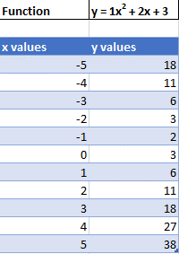
Set up your Table
- Create the Function that you want to graph
- Under the X Column, create a range. In this example, we’re range from -5 to 5
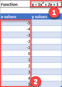
Fill in Y Column
Create a formula using the Function, substituting x with what is in Column B.
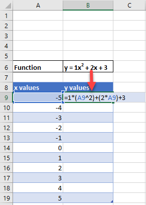
After using this formula for all the rows, you should have a table that looks like below.
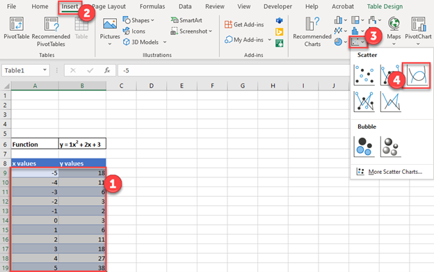
Creating Scatterplot
- Highlight Dataset
- Select Insert
- Select Scatterplot
- Select Scatter with Smooth Lines
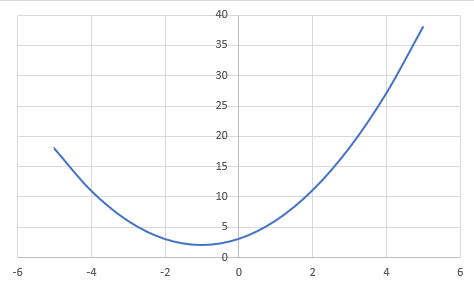
This will create a graph that should look similar to below.
Add Equation Formula to Graph
- Click Graph
- Select Chart Design
- Click Add Chart Element
- Click Trendline
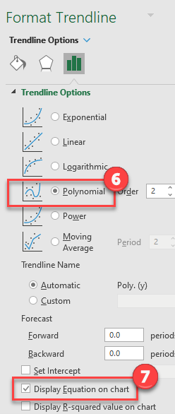
- Select More Trendline Options
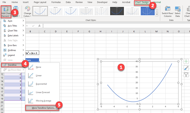
6. Select Polynomial
7. Check Display Equation on Chart
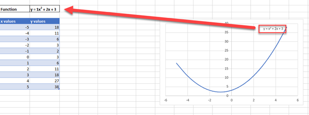
Final Scatterplot with Equation
Your final equation on the graph should match the function that you began with.
How to Graph an Equation / Function in Google Sheets
Creating a Scatterplot
- Using the same table that we made as explained above, highlight the table
- Click Insert
- Select Chart
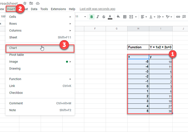
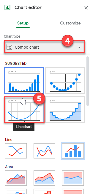
4. Click on the dropdown under Chart Type
5. Select Line Chart
Adding Equation
- Click on Customize
- Select Series
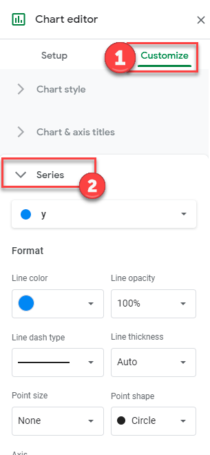
3. Check Trendline
4. Under Type, Select Polynomial
5. Under Label, Select Use Equation
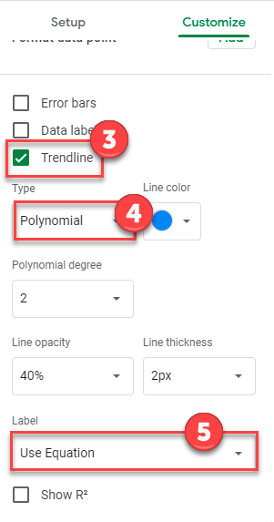
Final Scatterplot with Equation
As you can see, similar to the exercise in Excel, the equation matches the function that we began with.
Источник
Варианты построения графика функции в Microsoft Excel

Вариант 1: График функции X^2
В качестве первого примера для Excel рассмотрим самую популярную функцию F(x)=X^2. График от этой функции в большинстве случаев должен содержать точки, что мы и реализуем при его составлении в будущем, а пока разберем основные составляющие.
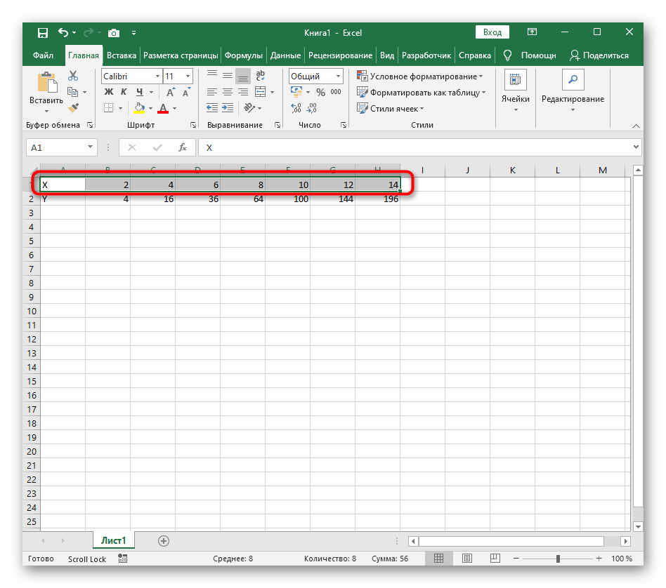
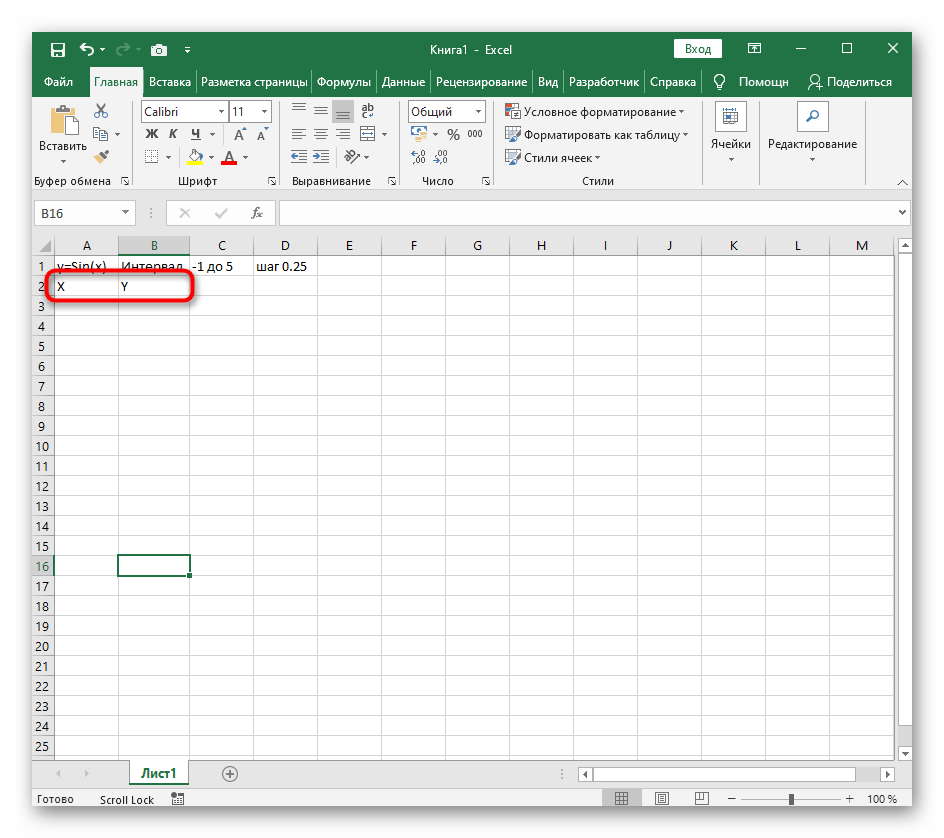
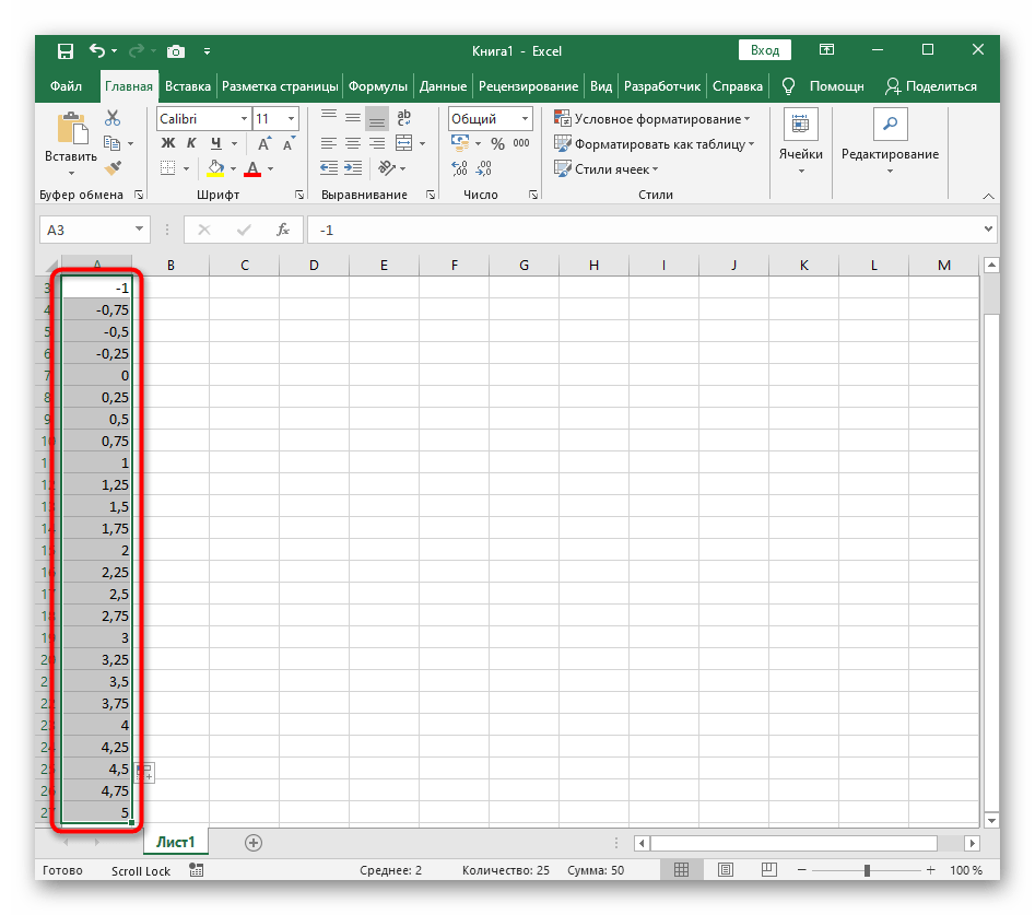
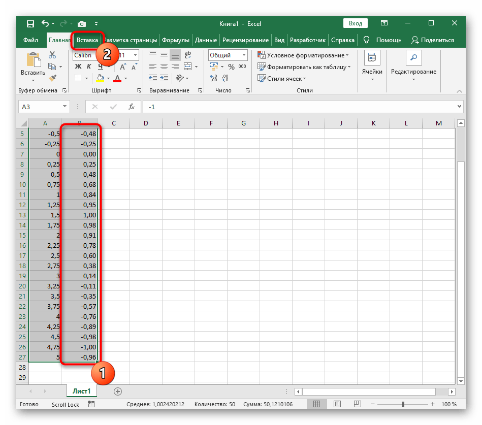
- Создайте строку X, где укажите необходимый диапазон чисел для графика функции.
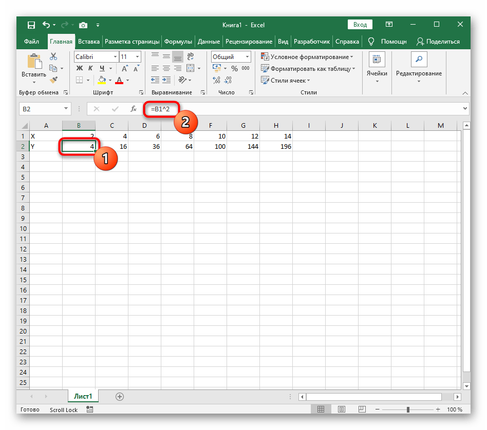
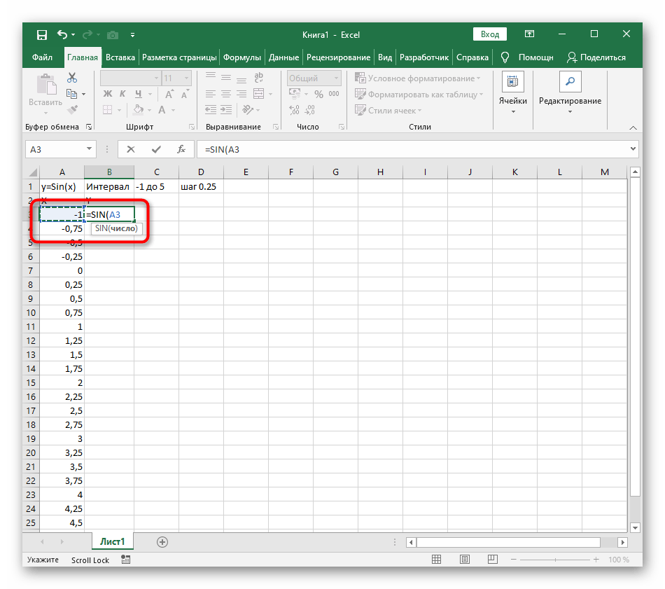
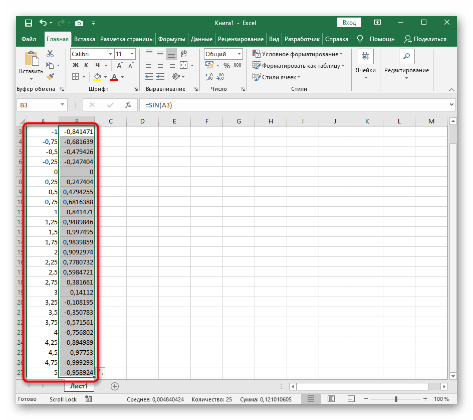
- Ниже сделайте то же самое с Y, но можно обойтись и без ручного вычисления всех значений, к тому же это будет удобно, если они изначально не заданы и их нужно рассчитать.
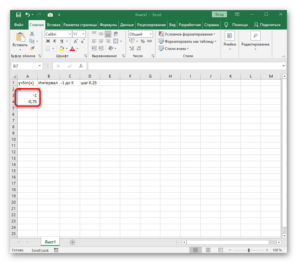
- Нажмите по первой ячейке и впишите =B1^2 , что значит автоматическое возведение указанной ячейки в квадрат.

Если график должен быть точечным, но функция не соответствует указанной, составляйте его точно в таком же порядке, формируя требуемые вычисления в таблице, чтобы оптимизировать их и упростить весь процесс работы с данными.
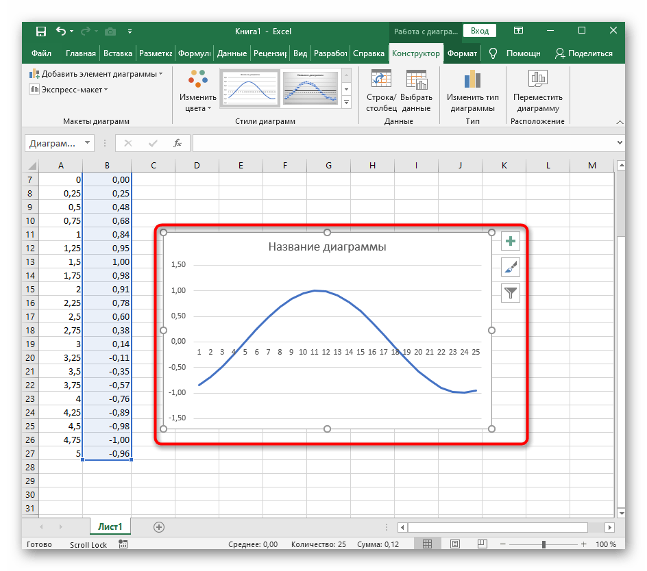
Вариант 2: График функции y=sin(x)
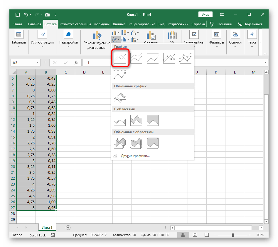
Функций очень много и разобрать их в рамках этой статьи просто невозможно, поэтому в качестве альтернативы предыдущему варианту предлагаем остановиться на еще одном популярном, но сложном — y=sin(x). То есть изначально есть диапазон значений X, затем нужно посчитать синус, чему и будет равняться Y. В этом тоже поможет созданная таблица, из которой потом и построим график функции.

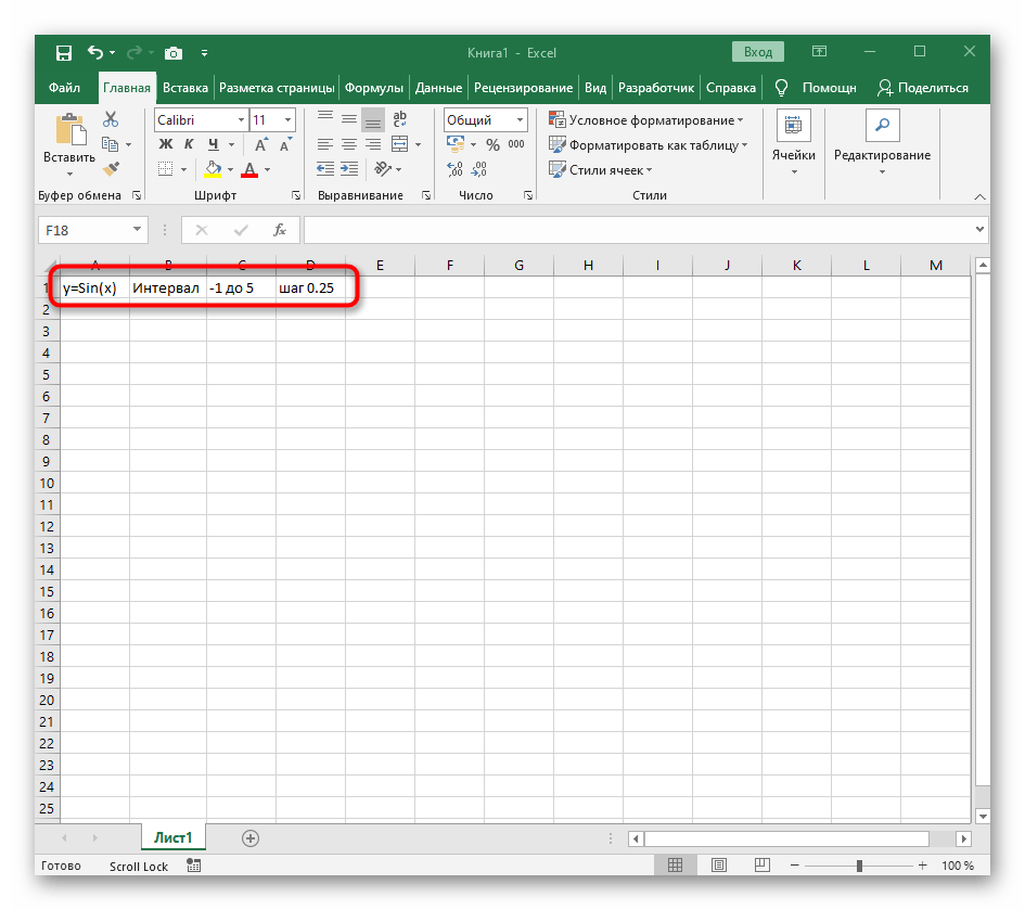
- Для удобства укажем всю необходимую информацию на листе в Excel. Это будет сама функция sin(x), интервал значений от -1 до 5 и их шаг весом в 0.25.
Источник
Plots in Excel
Plots in Excel (Table of Contents)
Introduction to Plots in Excel
Plots are charts andn graphs which are used to visualize and interpret data so that values for two different variables can be represented along the two axes (horizontal axis, i.e. the x axis and vertical axis, i.e. the y axis). Plots are basically scatter charts generally used to show a graphical relationship between two variables
Excel functions, formula, charts, formatting creating excel dashboard & others
Scatter plots use the Cartesian axes or coordinates so as to display the two data sets’ values.
In MS Excel, some layouts that are available for scatter plot are:
- Simple Scatter plot.
- Scatter with smooth lines and markers.
- Scatter with smooth lines.
- Scatter with straight lines and markers.
- Scatter with straight lines.
- Bubble chart.
- 3-D Bubble chart.
We can interpret the scatter plots in the following manner:
- If the data points on the plot look like they are randomly scattered, then it implies that there is no correlation between the two variables.
- If the data points on a plot are spread widely on the plane, then it implies that the correlation between two variables is weak.
- The correlation between two variables is said to be strong if the data points are concentrated around a line on the plot.
- The correlation between two datasets is positive If the data points’ pattern on the plot goes from lower left to upper right
- The correlation between two datasets is negative if the data points’ pattern on the plot goes from upper left to lower right,
Examples of Plots in Excel
Lets us discuss the examples of Plots in Excel.
Example #1 – Simple Scatter Plot
Let us suppose there is an interrelated dataset where we have some people’s monthly salaries and their expenditures. Now the relation between salary and expenditure can be plotted in Excel with the help of a scatter plot.
We have the following data of monthly salaries and expenditures in an Excel file:
Now in order to create a scatter plot for this data in Excel, the following steps can be used:
- Select the dataset and click on the ‘Insert’ tab. Now select ‘Scatter Chart’:
- With this, we will have the data plotted as follows:
Now the chart title can be changed by double-clicking on it and then renaming it:
- Now right click on the scatter lot -> Click on ‘Select Data’:
- On doing this, we will get a popup window:
- In the resulting window, select ‘Salary’ in the section: ‘Legend Entries’, and then select‘Remove’.
- Now in the section ‘Legend Entries’, select ‘Expenditure’ in this window, and choose ‘Edit’ :
- With this, we will have a popup window for the edit series:
- Now in this ‘Edit Series’ window, select ‘Salary’ range under ‘Series X values’:
- This will finally generate the below scatter plot:
- Now right-click on any data point or dot) -> Select ‘Format data Series’:
- With this, we will have a ‘Format Series’ dialog box. In this, click on ‘Effects’ and choose ‘3-D Format’:
- Now under ‘3-D Format’, select ‘circle’ type top level:
- Now in the ‘Format Series’, choose ‘Fill & Line’ and select ‘Marker’:
- Expand the ‘Fill’ option in the ‘Marker’ section -> Select ‘Vary colors by point’:
With this, each dot or data point will be represented with a different colour
- Now expand ‘Marker Options’ in the ‘Marker’ section. Choose ‘Built-in’ and then increase the value of size:
With this, the data points’ size will be increased.
- Now on the right of the plot, click on the ‘Plus’ icon in order to open the ‘Chart Elements’ dialog box:
- Now check mark ‘Axis Titles’in the ‘Chart Elements’ dialog box. On doing this,we will have an ‘Axis Title’ textbox on both the axes. (horizontal and vertical
Источник
Excel 2016, как известно, обогатился новыми типами диаграмм. Одна такая, которая диаграмма Парето, уже была показана. В этот раз рассмотрим другую, чисто статистическую. Называется «ящик с усами» или «коробчатая диаграмма» (box-and-whiskers plot или boxplot).
Раньше я такие видел только в специализированных ПО, типа STATISTICA, и для того, чтобы нарисовать подобную диаграмму в Excel, нужно было изрядно потрудиться. Теперь она есть в стандартном наборе Excel.

Зачем нужна такая диаграмма? Допустим, есть выборка для анализа. А еще лучше несколько выборок, которые нужно сравнить. Для этого рассчитывают различные показатели. Однако к любому расчету всегда хочется добавить наглядности, чтобы мозг перешел в режим образного представления, а не довольствовался сухими цифрами и формулами. Поэтому основные характеристики ловко изображают на рисунке. Отличным вариантом будет как раз диаграмма «ящик с усами».

На рисунке показан формат по умолчанию. Как видно, сравниваются две выборки путем изображения двух «ящиков с усами».
Что здесь что обозначает?
Крестик посередине – это среднее арифметическое по выборке.
Линия чуть выше или ниже крестика – медиана.
Нижняя и верхняя грань прямоугольника (типа ящика) соответствует первому и третьему квартилю (значениям, отделяющим ¼ и ¾ выборки). Расстояние между 1-м и 3-м квартилем – это межквартильный размах (или расстояние).
Горизонтальные черточки на конце «усов» – максимальное и минимальное значение (без учета выбросов, см. ниже).
Отдельные точки – это выбросы, которые показываются по умолчанию. Если значение выходит за пределы 1,5 межквартильных размаха от ближайшего квартиля, то оно считается аномальным. Их можно скрыть (см. ниже настройки).
Во всей красе «ящик с усами» проявляется при сравнении выборок, в которых данные делятся на категории. Допустим, провели некоторый эксперимент среди мужчин и женщин. Есть данные до и после эксперимента по обоим полам. Для анализа потребуется вычислить различные показатели. А если к этому добавить диаграмму «ящик с усами», то результат будет весьма наглядным.

Отлично видно, что после проведения эксперимента данные по мужчинам в целом уменьшились, а данные среди женщин наоборот, увеличились. Это не значит, что выборки больше не нужно анализировать (сравнивать, проверять гипотезы и т.д.). Но наглядность сильно улучшает понимание. Перейдем к настройкам.
Настройки диаграммы «ящик с усами»
Общий вид диаграммы настраивается стандартно. Можно менять цвет, добавлять подписи и т.д. Для этого есть две контекстные вкладки на ленте (Конструктор и Формат). Но есть настройки, предназначенные специально для этой диаграммы.
Выбираем какой-либо ряд и жмем Ctrl+1. Либо два раза кликаем по какому-нибудь «ящику». Можно через правую кнопку Формат ряда данных…. Справа вылазит панель настроек.

Рассмотрим по порядку.
Боковой зазор – регулирует ширину ящиков и расстояние между ними.
Показывать внутренние точки. Если поставить галочку, то на оси, где расположены «усы», точками будут показаны все значения. Так хорошо видно распределение внутри групп.

Показывать точки выбросов – отражать экстремальные значения.

Выбросы – это точки, выходящие за пределы 1,5 межквартильных размаха.
Показать средние метки – среднее арифметическое (крестики). Стоят по умолчанию, но можно скрыть.
Показать среднюю линию – только для различных категорий. Показывает изменения по категориям.

Если добавить линии, то изменения после эксперимента станут видны еще лучше. В справке написано, что соединяются медианы, но на графике почему-то соединяются средние. Чудеса.
Инклюзивная медиана или эксклюзивная медиана. Инклюзивная медиана включает в «ящик» квартильные значения , а эксклюзивная медиана не включает. При выборе «эксклюзивной медианы» верх и низ «ящика» соответствует средней между квартильным и следующим (от центра) значением. По умолчанию стоит «эксклюзивная». Пусть стоит дальше. Причем тут медиана, вообще не понял, – речь ведь про квартиль. Думал, криво перевели, но в английской версии те же названия. В общем, здесь лучше ничего не менять.
Своевременное использование диаграммы «ящик-усы» может дать весьма ценную и наглядную информацию. Аналитику, который использует специализированные программы или трудоемкие настройки Excel, будет очень приятно иметь такую диаграмму под рукой.
Как показано в ролике ниже, все делается очень быстро и просто.
Поделиться в социальных сетях:
Excel has some useful chart types that can be used to plot data and show analysis.
A common scenario is where you want to plot X and Y values in a chart in Excel and show how the two values are related.
This can be done by using a Scatter chart in Excel.
For example, if you have the Height (X value) and Weight (Y Value) data for 20 students, you can plot this in a scatter chart and it will show you how the data is related.
Below is an example of a Scatter Plot in Excel (also called the XY Chart):

In this tutorial, I will show you how to make a scatter plot in Excel, the different types of scatter plots, and how to customize these charts.
What is a Scatter Chart and When To Use It?
Scatter charts are used to understand the correlation (relatedness) between two data variables.
A scatter plot has dots where each dot represents two values (X-axis value and Y-axis value) and based on these values these dots are positioned in the chart.
A real-life example of this could be the marketing expense and the revenue of a group of companies in a specific industry.
When we plot this data (Marketing Expense vs. Revenue) in a scatter chart, we can analyze how strongly or loosely these two variables are connected.
Creating a Scatter Plot in Excel
Suppose you have a dataset as shown below and you want to create a scatter plot using this data.

The aim of this chart is to see whether there is any correlation between the marketing budget and the revenue or not.
For making a scatter plot, it’s important to have both the values (of the two variables that you want to plot in the scatter chart) in two separate columns.
The column on the left (Marketing Expense column in our example) would be plotted on the X-Axis and the Revenue would be plotted on the Y-Axis.
Below are the steps to insert a scatter plot in Excel:
- Select the columns that have the data (excluding column A)

- Click the Insert option

- In the Chart group, click on the Insert Scatter Chart icon
- Click on the ‘Scatter chart’ option in the charts thats show up

The above steps would insert a scatter plot as shown below in the worksheet.
The column on the left (Marketing Expense column in our example) would be plotted on the X-Axis and the Revenue would be plotted on the Y-Axis. It’s best to have the independent metric in the left column and the one for which you need to find the correlation in the column on the right.
Adding a Trend Line to the Scatter Chart
While I will cover more ways to customize the scatter plot in Excel later in this tutorial, one thing that you can do immediately after building the scatter plot is to add a trend line.
It helps you quickly get a sense of whether the data is positively or negatively correlated, and how tightly/loosely correlated it is.
Below are the steps to add a trendline to a scatter chart in Excel:
- Select the Scatter plot (where you want to add the trendline)
- Click the Chart Design tab. This is a contextual tab which only appears when you select the chart

- In the Chart Layouts group, click on the ‘Add Chart Element’ option

- Go to the ‘Trendline’ option and then click on ‘Linear’

The above steps would add a linear trendline to your scatter chart.

Just by looking at the trendline and the data points plotted in the scatter chart, you can get a sense of whether the data is positively correlated, negatively correlated, or not correlated.
In our example, we see a positive slope in the trendline indicating that the data is positively correlated. This means that when the marketing expenses go up then the revenue goes up and if the marketing expenses go down then the revenue goes down.
In case the data is negatively correlated, then there would be an inverse relation. In that case, if the marketing expenses go up then the revenue would go down and vice versa.
And then there is a case where there is no correlation. In this case, when the marketing expenses increase, their revenue may or may not increase.
Note that the slope only tells us whether the data is positively or negatively correlated. it doesn’t tell us how closely it’s related.
For example, in our example, by looking at the trendline we cannot say how much the revenue will go up when the marketing expense increases by 100%. This is something that can be calculated using the correlation coefficient.
You can find that using the below formula:
=CORREL(B2:B11,C2:C11)
The correlation coefficient varies between -1 and 1, where 1 would indicate a perfectly positive correlation and -1 would indicate a perfectly negative correlation
In our example, it returns 0.945, indicating that these two variables have a high positive correlation.
Identifying Clusters using Scatter Chart (Practical Examples)
One of the ways I used to use scatter charts in my work as a financial analyst was to identify clusters of data points that exhibit a similar kind of behavior.
This usually works well when you have a diverse data set with less overall correlation.
Suppose you have a data set as shown below, where I have 20 companies with their revenue and profit margin numbers.

When I create a scatterplot for this data, I get something as shown below:

In this chart, you can see that the data points are all over the place and there is a very low correlation.
While this chart doesn’t tell us much, one way you can use it to identify clusters in the four quadrants in the chart.
For example, the data point in the bottom left quadrant are those companies where the revenue is low and the net profit margin is low, and the companies in the bottom right quadrant are those where the revenue is high but the net profit margin is low.
This used to be one of the highly discussed charts in the management meeting when we used to identify prospective customers based on their financial data.
Different Types of Scatter Plots in Excel
Apart from the regular scatter chart that I have covered above, you can also create the following scatter plot types in Excel:
- Scatter with Smooth Lines
- Scatter with Smooth Lines and Markers
- Scatter with Straight Lines
- Scatter with Straight Lines and Markers
All these four above scatter plots are suitable when you have fewer data points and when you’re plotting two series in the chart.
For example, suppose you have the Marketing Expense vs Revenue data as shown below and you want to plot a scatter with smooth lines chart.
Below are the steps to do this:
- Select the dataset (excluding the company name column)
- Click the Insert tab
- In the Charts group, click on the Insert Scatter Chart option
- Click on Scatter with Smooth Lines and Markers options

You will see something as shown below.

This chart can quickly become unreadable if you have more data points. This is why it is recommended to use this with fewer data points only.
I have never used this chart in my work as I don’t think it gives any meaningful insight (since we can’t plot more data points to it).
Customizing Scatter Chart in Excel
Just like any other chart in Excel, you can easily customize the scatter plot.
In this section, I will cover some of the customizations you can do with a scatter chart in Excel:
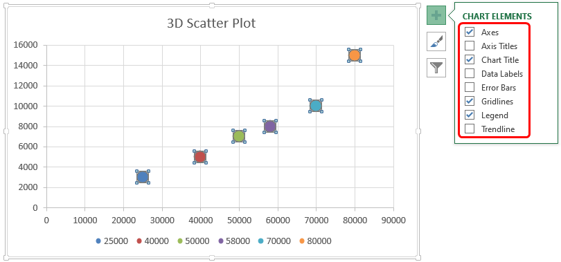
Adding / Removing Chart Elements
When you click on the scatter chart, you will see plus icon at the top right part of the chart.
When you click on this plus icon, it will show you options that you can easily add or remove from your scatter chart.
Here are the options that you get:
- Axes
- Axis Title
- Chart Title
- Data Labels
- Error Bars
- Gridlines
- Legend
- Trendlines
Some of these options are already present in your chart, and you can remove these elements by clicking on the checkbox next to the option (or add these by clicking the checkbox if not checked already).
For example, if I want to remove the Chart Title, I can simply uncheck the option and it would be gone,
In case you need more control, you can click on the little black arrow that appears when you hover the cursor hover over any of the options.

Clicking on it will give you more options for that specific chart element (these open as a pane on the right side).
Note: All the screenshots I have shown you are from a recent version of Excel (Microsoft 365). In case you’re using an older version, you can get the same options when you right-click on any of the chart elements and click on the Format option.
Let’s quickly go through these elements and some of the awesome customizations you can do to scatter charts using it.
Axes
Axes are the vertical and horizontal values that you see right next to the chart.
One of the most useful customizations you can do with axes is to adjust the maximum and minimum value it can show.
To change this, right-click on the axes in the chart and then click on Format axes. This will open the Format Axis pane.

In the Axis option, you can set the minimum and maximum bounds as well as the major and minor units.

In most cases, you can set this to automatic, and Excel will take care of it based on the dataset. But in case you want specific values, you can change them from here.
One example could be when you don’t want the minimum value in the Y-axis to be 0, but something else (say 1000). Changing the lower bound to 1000 will adjust the chart so that the minimum value in the vertical axis would then be 1000.
Axis Title
The Axis title is something you can use to specify what the X and Y-axis represent in the scatter chart in Excel.
In our example, it would be the Net Income for the X-axis and Marketing Expense for the Y-axis.
You can choose to not show any axis title, and you can remove these by selecting the chart, clicking on the plus icon, and then unchecking the box for Axis title.

To change the text in the axis title, simply double-click on it and then type whatever you want as the axis title.
You can also link the Axis title value to a cell.
For example, if you want the value in cell B1 to show up in the vertical axis title, click on the axis title box and then enter =B1 in the formula bar. This will show the value in cell B1 in the axis title.
You can do the same for the horizontal axis title and link it to a specific cell. This makes these titles dynamic and if the cell value changes, the axis titles will also change.
If you need more control on formatting the axis titles, click on any axis, right-click and then click on Format Axis Title.

With these options, you can change the fill and border of the title, change the text color, alignment, and rotation.

Chart Title
Just like Axis titles, you can also format the Chart title in a scatter plot in Excel.
A chart title is usually used to describe what the chart is about. For example, I can use ‘Marketing Expense Vs Revenue’ as the chart title.

If you don’t want the chart title, you can click and delete it. And in case you don’t have it, select the chart, click on the plus icon and then check the Chart Title option.

To edit the text in the Chart title, double-click on the box and manually type the text you want there. And in case you want to make the chart title Dynamic, you can click the title box and then type the cell reference or the formula in the formula bar.
To format the chart title, right-click on the Chart Title and then click on the ‘Format Chart Title’ option. This will show the Format Chart Title pane on the right.

With these options, you can change the fill and border of the title, change the text color, alignment, and rotation.

Data Labels
By default, data labels are not visible when you create a scatter plot in Excel.
But you can easily add and format these.
Do add the data labels to the scatter chart, select the chart, click on the plus icon on the right, and then check the data labels option.

This will add the data labels that will show the Y-axis value for each data point in the scatter graph.
To format the data labels, right-click on any of the data labels and then click on the ‘Format Data Labels’ option.

This will open the former data labels pane on the right, and you can customize these using various options listed in the pane.
Apart from the regular formatting such as fill, border, text color, and alignment, you also get some additional label options that you can use.
In the ‘Label Contains’ options, you can choose to show both the X-axis and the Y-axis value, instead of just the Y-axis.

You can also choose the option ‘Value from Cells’. which will allow you to have data labels that are there in a column in the worksheet (it opens a dialog box when you select this option and you can choose a range of cells whose values would be displayed in the data labels. In our example, I can use this to show company names in the data labels

You can also customize the position of the label and the format in which it’s shown.
Error Bars
While I have not seen error bars being used in scatter charts, Excel does have an option that allows you to add these error bars for each data point in the scatterplot in Excel.
To add the error bars, select the chart, click on the plus icon, and then check the Error Bars option.

And if you want to customize these error bars further, right-click on any of these error bars and then click on the ‘Format Error Bars’ option.

This will open the ‘Format Error Bars’ pane on the right, where you can customize things such as color, direction, and style of the error bars.

Gridlines
Gridlines are useful when you have a lot of data points on your chart as it allows the reader to quickly understand the position of the data point.
When you create a scatterplot in Excel, gridlines are enabled by default.
You can format these gridlines by right-clicking on any of the gridlines and clicking on the Format Gridlines option.

This will open the Format Gridlines pane on the right way you can change the formatting such as the color, thickness, of the gridline.
Apart from the major gridlines that are already visible when you create the scatter diagram, you can also add minor gridlines.
Between two major gridlines, you can have a few minor gridlines that further improve the readability of the chart in case you have a lot of data points.
To add minor horizontal or vertical gridlines, select the chart, click the plus icon, and hover the cursor over the Gridlines option.
Click the thick black arrow there appears and then check the ‘Primary Minor Horizontal’ or ‘Primary Minor Vertical’ option to add the minor gridlines

Legend
If you have multiple series plotted in the scatter chart in Excel, you can use a legend that would denote what data point refers to what series.
By default, there is no legend when you create a scatter chart in Excel.
To add a legend to the scatter chart, select the chart, click the plus icon, and then check the legend option.

To format the legend, right-click on the legend that appears and then click on the ‘Format Legend’ option.

In the Format Legend pane that opens up, you can customize the fill color, border, and position of the legend in the chart.

Trendline
You can also add a trendline in the scatter chart that would show whether there is a positive or negative correlation in the data set.
I’ve already covered how to add a trendline to a scatter chart in Excel in one of the sections above.
3D Scatter Plot in Excel (are best avoided)
Unlike a Line chart, Column chart, or Area chart, there is no inbuilt 3D scatter chart in Excel.
While you can use third-party add-ins and tools to do this, I cannot think of any additional benefit that you will get with a 3D scatter chart as compared to a regular 2D scatter chart.
In fact, I recommend staying away from any kind of 3D chart as it has the potential of misrepresenting the data and portions in the chart.
So this is how you can create a scatter plot in Excel and customize it to make it fit your brand and requirements.
I hope you found this tutorial useful.
Other Excel tutorials you may also like:
- How to Spot Data Point in Excel Scatter Chart
- KPI Dashboard in Excel – Extract List of Companies from the Scatter Chart
- How to Make a PIE Chart in Excel
- How to Create an Area Chart in Excel
- How to Create Combination Charts in Excel
- Creating Actual vs Target Chart in Excel
- Calculate Area Under Curve in an Excel