
- Стиль запятой в Excel
Стиль запятой в Excel (Содержание)
- Стиль запятой в Excel
- Как применить стиль запятой в Excel?
Стиль запятой в Excel
Внешний вид числового значения или чисел, введенных в ячейку Excel, можно изменить различными способами. По умолчанию, в ваших данных о продажах или любых числовых значениях в Excel не отображаются запятые или первые два десятичных знака для ваших записей в конце, так что становится очень трудно читать и анализировать числа или числовые значения. В Excel имеются различные встроенные числовые форматы для процентных, числовых или числовых значений, валюты, даты и времени.
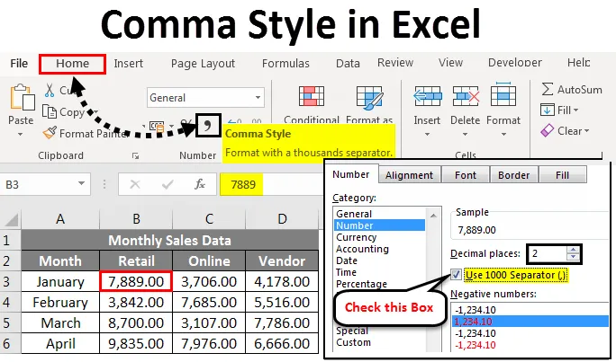
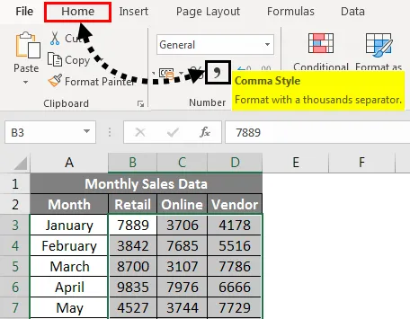
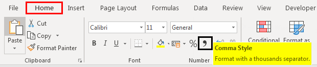
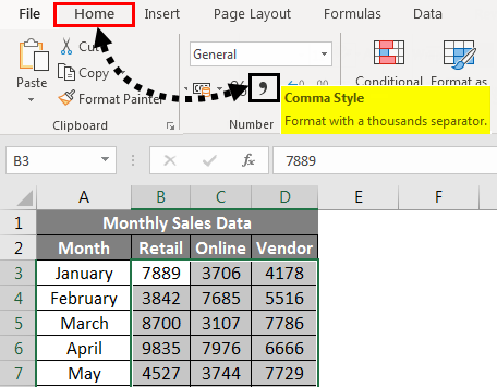
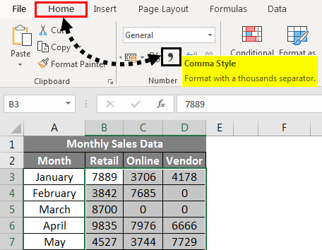
Формат стиля запятой классифицируется в разделе « Числовой формат» на вкладке « Главная ».
Формат в стиле запятой также называется разделителем тысяч.
Этот формат будет очень полезен, когда вы работаете с большой таблицей данных о финансовых продажах (ежеквартальные или полугодовые или годовые данные о продажах), здесь применяется формат в стиле запятой, а числа выглядят лучше. Он используется для определения поведения цифр по отношению к тысячам или недостаткам, миллионам или миллиардам цифр. Формат Comma Style предлагает хорошую альтернативу формату Currency. Формат в стиле запятой вставляет запятые в большем количестве, чтобы разделить тысячи, сотни тысяч, миллионы, миллиарды и так далее.
Стиль запятой — это тип числового формата, в котором он добавляет запятые к большим числам, добавляет два десятичных знака (т. Е. 1000 становится 1000, 00), отображает отрицательные значения в закрытых скобках и представляет нули с тире (-).
Сочетание клавиш для стиля запятой ALT + HK

Прежде чем приступить к работе с форматом чисел в стиле запятых, нам нужно проверить, включены ли десятичные разделители и разделители тысяч или нет в Excel. Если он не включен, нам нужно включить его и обновить, выполнив следующие действия.
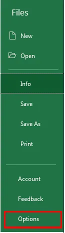
- Чтобы проверить десятичные разделители и разделители тысяч в Excel, перейдите на вкладку « Файл ».

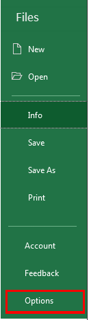
- Нажмите « Параметры» в списке элементов слева, появится диалоговое окно «Параметры Excel».
- В диалоговом окне «Параметры Excel». Нажмите кнопку « Дополнительно» в списке элементов слева.
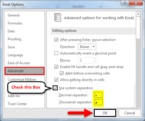
- Под опциями редактирования, нажмите или отметьте флажок Использовать системные разделители, если в поле нет флажка. Окна редактирования десятичного разделителя и разделителя тысяч отображаются после того, как вы установите флажок «Использовать разделители системы». Здесь я выбрал запятую в качестве разделителя тысяч и точку в качестве десятичного разделителя. После этого нажмите ОК .

Эти разделители автоматически вставляются во все числа в вашей рабочей книге при использовании числового формата в стиле запятой.
Ниже приведены различные типы числовых значений или типов чисел, которые встречаются в данных о продажах.
- положительный
- отрицательный
- Нуль
- Текст
Как применить стиль запятой в Excel?
Давайте посмотрим, как работает числовой формат в виде запятой для различных типов числовых значений или числовых типов в Excel.
Вы можете скачать этот шаблон Excel в стиле запятой здесь — Шаблон в стиле запятой Excel
Стиль запятой в Excel — Пример № 1
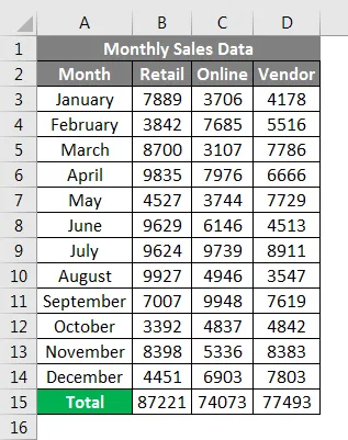
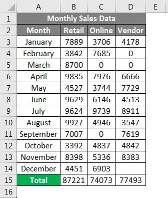
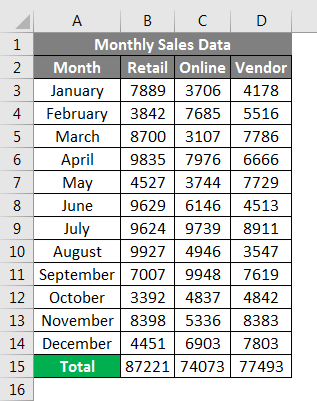
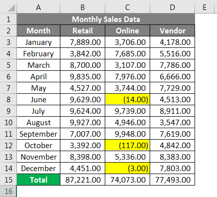
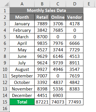
В приведенном ниже примере у меня есть данные о месячных продажах компании, которые ежемесячно содержат данные о розничных продажах, онлайн-продажах и продажах поставщиков. В этих необработанных данных о продажах внешний вид данных не применяется ни к какому числовому формату.
Итак, мне нужно применить формат чисел в стиле запятой для этих положительных продаж.
Чтобы отобразить номера продаж в формате запятой в Excel:
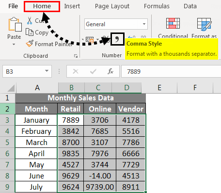
- Выберите ячейки, содержащие числовые значения продаж, для которых я хочу отображать числа в формате чисел в стиле запятой.
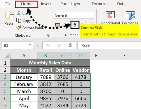
- На вкладке « Главная » в группе « Число » вы можете выбрать символ запятой и щелкнуть по команде «Стиль запятой».
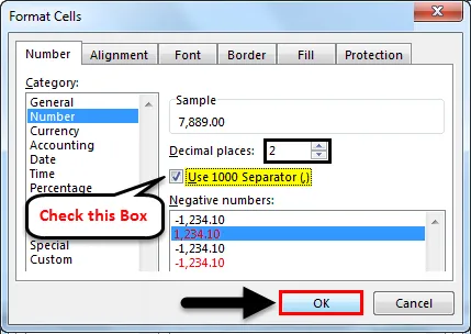
Или это можно сделать другим способом, т. Е. Как только вы выберете числовые значения продаж, затем щелкните правой кнопкой мыши, выберите « Формат ячеек». После того, как появится это окно, в разделе « Числа» необходимо выбрать « Число» в категории и установить флажок « Использовать разделитель 1000» и в десятичных разрядах введите значение 2 и нажмите ОК .
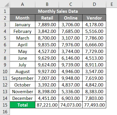
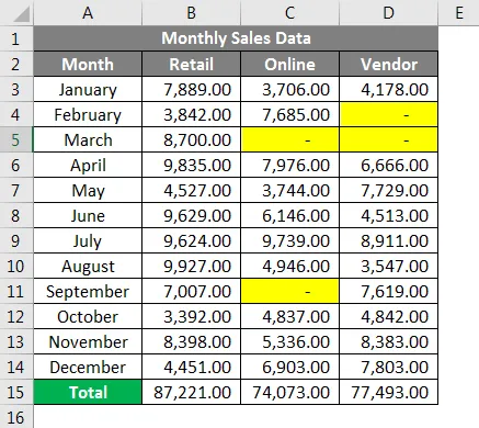
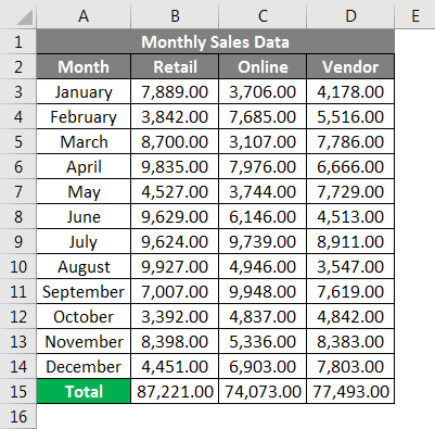
После того, как вы нажали кнопку «Стиль запятой», вы можете увидеть изменения в продажной стоимости, где Excel разделяет тысячи запятой и добавляет два десятичных знака в конце.
В первой ячейке вы можете наблюдать, где 7889 становится 7 889, 00. Результат показан ниже.
Стиль запятой в Excel — Пример № 2
В приведенном ниже примере у меня есть данные о ежемесячных продажах компании, которые ежемесячно содержат данные о розничных продажах, онлайн-продажах и продажах поставщиков, в этих исходных данных о продажах они содержат как положительные, так и отрицательные значения . В настоящее время внешний вид данных о продажах не имеет никакого числового формата.
Итак, мне нужно применить формат чисел в стиле запятой для этих положительных и отрицательных значений.

Чтобы отобразить числа в формате запятой в Excel:
- Выберите ячейки, содержащие числовые значения продаж, для которых я хочу отображать числа в формате чисел в стиле запятой. На вкладке «Главная» в группе «Число» вы можете выбрать символ запятой и щелкнуть команду «Стиль запятой».
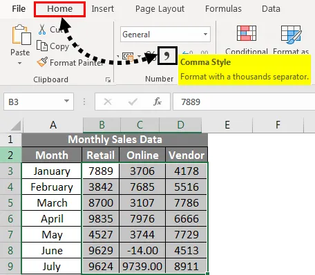
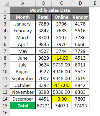
- После того, как вы нажали кнопку « Стиль запятой », вы можете увидеть изменения в продажной стоимости.

Где Excel отделяет тысячи запятыми и добавляет два десятичных знака в конце, и это заключает отрицательные значения продаж в закрытой паре скобок
Стиль запятой в Excel — Пример № 3
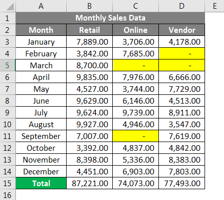
В приведенном ниже примере у меня есть данные о ежемесячных продажах компании, которые ежемесячно содержат данные о розничных продажах, онлайн-продажах и продажах поставщиков, в этих исходных данных о продажах они содержат как положительные, так и нулевые значения . В настоящее время внешний вид данных о продажах не имеет никакого числового формата.
Итак, мне нужно применить формат чисел в стиле запятой для этих положительных и нулевых значений.
Чтобы отобразить числа в формате запятой в Excel:
- Выберите ячейки, содержащие числовые значения продаж, для которых я хочу отображать числа в формате чисел в стиле запятой. На вкладке « Главная » в группе «Число» вы можете выбрать символ запятой и щелкнуть команду «Стиль запятой».
После того, как вы нажмете кнопку « Стиль запятой », вы сможете увидеть изменения в продажной стоимости.
Где Excel отделяет тысячи запятой и добавляет два десятичных знака в конце, а нулевые значения представляются символом тире.
То, что нужно запомнить
- Номер в стиле запятой Форматирование в Excel облегчает доступ к вашим данным и их удобочитаемость, а также помогает настроить данные о продажах в соответствии с отраслевым стандартом.
- Помимо различных опций формата чисел в Excel, вы можете создать свой собственный формат чисел в Excel на основе вашего выбора.
Рекомендуемые статьи
Это было руководство по стилю запятой в Excel. Здесь мы обсудили, как применить Comma Style в Excel вместе с практическими примерами и загружаемым шаблоном Excel. Вы также можете просмотреть наши другие предлагаемые статьи —
- Как изменить формат даты в Excel?
- Форматирование данных в Excel
- Как объединить ячейки в Excel?
- Как обернуть текст в Excel?
Содержание
- How to add comma in Excel column between names
- Стиль запятой в Excel — Как применить стиль запятой в Excel?
- Стиль запятой в Excel
- Как применить стиль запятой в Excel?
- Стиль запятой в Excel — Пример № 1
- Стиль запятой в Excel — Пример № 2
- Стиль запятой в Excel — Пример № 3
- То, что нужно запомнить
- Рекомендуемые статьи
- Comma Style in Excel
- Comma Style Formatting in Excel
- How to Apply Comma Style in Excel (accounting format)?
- Excel Shortcuts to Use Comma Style Format
- Advantages
- Disadvantages
- Things to Remember
- Recommended Articles
How to add comma in Excel column between names
A free Office suite fully compatible with Microsoft Office
A free Office suite fully compatible with Microsoft Office
Excel uses the comma style to separate different lengths of numbers, such as hundreds, thousands, millions, etc. Users are able to read and spell the numbers incorrectly because to this. Select Format Cells from the right-click menu, then check the option next to Use 1000 separator in the Number section to enable the comma in any cell (,). In the number part of the Home menu ribbons, we may also utilise the comma style. To apply comma style, we can also utilise shortcut keys by hitting ALT + H + K at the same time. The Home tab’s Number format area is where you’ll find the comma style format.
The thousands separator is another name for the comma style format.
When working on a large table of financial sales data (quarterly, half-yearly, or annual sales data), this format will be quite useful since it applies a comma-style structure, which makes the figures seem nicer. It is used to describe how individual digits behave in respect to groups of thousands, millions, or billions of other digits. A decent substitute for the currency format is the comma style format. To separate thousands, hundred thousand, millions, billions, and other huge figures, the comma style format adds commas. A sort of number format known as comma style adds commas to huge numbers, rounds decimal digits up to two places (so that 1000 becomes 1,000.00), shows negative values in closed parenthesis, and denotes zeros with a dash (-).
ALT + HK is the shortcut key for comma style.
Checking if decimal & thousand separators are enabled or not in Excel is necessary before working on comma style number format. If it is not enabled, we must activate it and update it using the procedures listed below.
1.Click the File tab in Excel to verify decimal and thousands of separators.
2. The Excel Options dialogue box opens when you select Options from the list of items on the left.
3. Excel Options dialogue box. In the list of options on the left, select Advanced.
4. If the Use system separators checkbox is not already checked, choose it by clicking or ticking it under the editing options. Once you choose the Use system separators checkbox, the Decimal separator and Thousands separator edit boxes appear. The thousands separator in this case was a comma, and the decimal separator was a full point. Click OK after that.
5. When you utilise the comma style number format, these separators are automatically added to all the numbers in your worksheet.
How to apply comma in excel
In the example shown below, I have monthly sales data from a firm that includes retail, online, and vendor sales statistics on a monthly basis. In this raw sales data, there is no numerical format added to the data’s presentation.
Therefore, for these positive sales amounts, I must use the comma style number format.
1.To show numbers in a comma style number format, select the cells that contain numeric sales data.
2. You may choose the comma symbol and click the Comma Style command in the Number group on the Home tab.
3. When you select the Comma Style option, Excel separates the thousands with a comma and adds two decimal places at the end. This alters the sales amount.
4. You can see that 603889 becomes 6,03,889 in the first cell. The outcome is displayed below.
Note: This was an attempt to show you how to add comma in excel online, 2016 and 2019, in both windows and mac.
To get the newest version of WPS Office, you must first access this operating interface.
You just need to have a little understanding of how and which way things work and you are good to go. With having this basic knowledge or information of how to use it, you can also access and use different other options on excel or spreadsheet. Also, it is very similar to Word or Document. So, in a way, if you learn one thing, like Excel, you can automatically learn how to use Word as well because both of them are very similar in so many ways. If you want to know more about WPS Office, you can download WPS Office to access, Word, Excel, PowerPoint for free.
Источник
Стиль запятой в Excel — Как применить стиль запятой в Excel?

Стиль запятой в Excel (Содержание)
- Стиль запятой в Excel
- Как применить стиль запятой в Excel?
Стиль запятой в Excel
Внешний вид числового значения или чисел, введенных в ячейку Excel, можно изменить различными способами. По умолчанию, в ваших данных о продажах или любых числовых значениях в Excel не отображаются запятые или первые два десятичных знака для ваших записей в конце, так что становится очень трудно читать и анализировать числа или числовые значения. В Excel имеются различные встроенные числовые форматы для процентных, числовых или числовых значений, валюты, даты и времени.
Формат стиля запятой классифицируется в разделе « Числовой формат» на вкладке « Главная ».

Формат в стиле запятой также называется разделителем тысяч.
Этот формат будет очень полезен, когда вы работаете с большой таблицей данных о финансовых продажах (ежеквартальные или полугодовые или годовые данные о продажах), здесь применяется формат в стиле запятой, а числа выглядят лучше. Он используется для определения поведения цифр по отношению к тысячам или недостаткам, миллионам или миллиардам цифр. Формат Comma Style предлагает хорошую альтернативу формату Currency. Формат в стиле запятой вставляет запятые в большем количестве, чтобы разделить тысячи, сотни тысяч, миллионы, миллиарды и так далее.
Стиль запятой — это тип числового формата, в котором он добавляет запятые к большим числам, добавляет два десятичных знака (т. Е. 1000 становится 1000, 00), отображает отрицательные значения в закрытых скобках и представляет нули с тире (-).
Сочетание клавиш для стиля запятой ALT + HK

Прежде чем приступить к работе с форматом чисел в стиле запятых, нам нужно проверить, включены ли десятичные разделители и разделители тысяч или нет в Excel. Если он не включен, нам нужно включить его и обновить, выполнив следующие действия.
- Чтобы проверить десятичные разделители и разделители тысяч в Excel, перейдите на вкладку « Файл ».

- Нажмите « Параметры» в списке элементов слева, появится диалоговое окно «Параметры Excel».

- В диалоговом окне «Параметры Excel». Нажмите кнопку « Дополнительно» в списке элементов слева.
- Под опциями редактирования, нажмите или отметьте флажок Использовать системные разделители, если в поле нет флажка. Окна редактирования десятичного разделителя и разделителя тысяч отображаются после того, как вы установите флажок «Использовать разделители системы». Здесь я выбрал запятую в качестве разделителя тысяч и точку в качестве десятичного разделителя. После этого нажмите ОК .

Эти разделители автоматически вставляются во все числа в вашей рабочей книге при использовании числового формата в стиле запятой.
Ниже приведены различные типы числовых значений или типов чисел, которые встречаются в данных о продажах.
Как применить стиль запятой в Excel?
Давайте посмотрим, как работает числовой формат в виде запятой для различных типов числовых значений или числовых типов в Excel.
Вы можете скачать этот шаблон Excel в стиле запятой здесь — Шаблон в стиле запятой Excel
Стиль запятой в Excel — Пример № 1
В приведенном ниже примере у меня есть данные о месячных продажах компании, которые ежемесячно содержат данные о розничных продажах, онлайн-продажах и продажах поставщиков. В этих необработанных данных о продажах внешний вид данных не применяется ни к какому числовому формату.
Итак, мне нужно применить формат чисел в стиле запятой для этих положительных продаж.

Чтобы отобразить номера продаж в формате запятой в Excel:
- Выберите ячейки, содержащие числовые значения продаж, для которых я хочу отображать числа в формате чисел в стиле запятой.
- На вкладке « Главная » в группе « Число » вы можете выбрать символ запятой и щелкнуть по команде «Стиль запятой».

Или это можно сделать другим способом, т. Е. Как только вы выберете числовые значения продаж, затем щелкните правой кнопкой мыши, выберите « Формат ячеек». После того, как появится это окно, в разделе « Числа» необходимо выбрать « Число» в категории и установить флажок « Использовать разделитель 1000» и в десятичных разрядах введите значение 2 и нажмите ОК .

После того, как вы нажали кнопку «Стиль запятой», вы можете увидеть изменения в продажной стоимости, где Excel разделяет тысячи запятой и добавляет два десятичных знака в конце.
В первой ячейке вы можете наблюдать, где 7889 становится 7 889, 00. Результат показан ниже.

Стиль запятой в Excel — Пример № 2
В приведенном ниже примере у меня есть данные о ежемесячных продажах компании, которые ежемесячно содержат данные о розничных продажах, онлайн-продажах и продажах поставщиков, в этих исходных данных о продажах они содержат как положительные, так и отрицательные значения . В настоящее время внешний вид данных о продажах не имеет никакого числового формата.
Итак, мне нужно применить формат чисел в стиле запятой для этих положительных и отрицательных значений.

Чтобы отобразить числа в формате запятой в Excel:
- Выберите ячейки, содержащие числовые значения продаж, для которых я хочу отображать числа в формате чисел в стиле запятой. На вкладке «Главная» в группе «Число» вы можете выбрать символ запятой и щелкнуть команду «Стиль запятой».

- После того, как вы нажали кнопку « Стиль запятой », вы можете увидеть изменения в продажной стоимости.

Где Excel отделяет тысячи запятыми и добавляет два десятичных знака в конце, и это заключает отрицательные значения продаж в закрытой паре скобок
Стиль запятой в Excel — Пример № 3
В приведенном ниже примере у меня есть данные о ежемесячных продажах компании, которые ежемесячно содержат данные о розничных продажах, онлайн-продажах и продажах поставщиков, в этих исходных данных о продажах они содержат как положительные, так и нулевые значения . В настоящее время внешний вид данных о продажах не имеет никакого числового формата.
Итак, мне нужно применить формат чисел в стиле запятой для этих положительных и нулевых значений.

Чтобы отобразить числа в формате запятой в Excel:
- Выберите ячейки, содержащие числовые значения продаж, для которых я хочу отображать числа в формате чисел в стиле запятой. На вкладке « Главная » в группе «Число» вы можете выбрать символ запятой и щелкнуть команду «Стиль запятой».

После того, как вы нажмете кнопку « Стиль запятой », вы сможете увидеть изменения в продажной стоимости.
Где Excel отделяет тысячи запятой и добавляет два десятичных знака в конце, а нулевые значения представляются символом тире.

То, что нужно запомнить
- Номер в стиле запятой Форматирование в Excel облегчает доступ к вашим данным и их удобочитаемость, а также помогает настроить данные о продажах в соответствии с отраслевым стандартом.
- Помимо различных опций формата чисел в Excel, вы можете создать свой собственный формат чисел в Excel на основе вашего выбора.
Рекомендуемые статьи
Это было руководство по стилю запятой в Excel. Здесь мы обсудили, как применить Comma Style в Excel вместе с практическими примерами и загружаемым шаблоном Excel. Вы также можете просмотреть наши другие предлагаемые статьи —
- Как изменить формат даты в Excel?
- Форматирование данных в Excel
- Как объединить ячейки в Excel?
- Как обернуть текст в Excel?
Источник
Comma Style in Excel


Comma Style Formatting in Excel
The comma style is a formatting style used in visualizing numbers with commas when the values are over 1,000. Such as, if we use this style on data with a value of 100,000, then the result displayed will be as (100,000). This formatting style can be accessed from the “Home” tab in the number section and click on the 1,000 (,) separator, known as the comma style in Excel.
For example, we have a company’s monthly sales and production dataset without a number format. In such cases, if we need to apply the comma style number format for the positive values, comma style formatting in Excel separates the thousands with a comma. It adds two decimal places at the end and a dash symbol at the zero values. It can also help create the custom number format of our choice. Moreover, it also makes it easier to access and increases readability by setting up data at an industry standard.
The comma style format (also known as the thousands separator) regularly goes with the “Accounting” format. Like the “Accounting” position, the comma arrangement embeds commas in bigger numbers to isolate thousands, hundred thousand, millions, and all values considered.
The standard comma style format contains up to two decimal points and a thousand separators and locks the dollar sign to the extreme left half of the cell. Negative numbers are shown in enclosures. To apply this format in a spreadsheet, we must feature every cell and click “Comma Style Format” under formatting choices in Excel Formatting Choices In Excel Formatting is a useful feature in Excel that allows you to change the appearance of the data in a worksheet. Formatting can be done in a variety of ways. For example, we can use the styles and format tab on the home tab to change the font of a cell or a table. read more .
You are free to use this image on your website, templates, etc., Please provide us with an attribution link How to Provide Attribution? Article Link to be Hyperlinked
For eg:
Source: Comma Style in Excel (wallstreetmojo.com)
How to Apply Comma Style in Excel (accounting format)?
Lets us start the below steps.
- We must first enter the values in Excel to use the comma number format in Excel.

We can use accounting Excel format in the Number format ribbon, select the amount cell, click on ribbon home, and select the Comma Style from the Number format column.
Once we click on the Comma Style, it will provide the comma-separated format value.

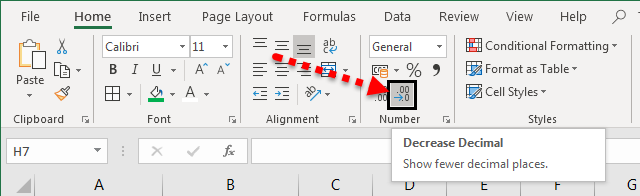
If we want to remove the decimal, we must click on the icon under Number on Decrease Decimal.
Once we remove the decimal, we can see below the value without decimals.

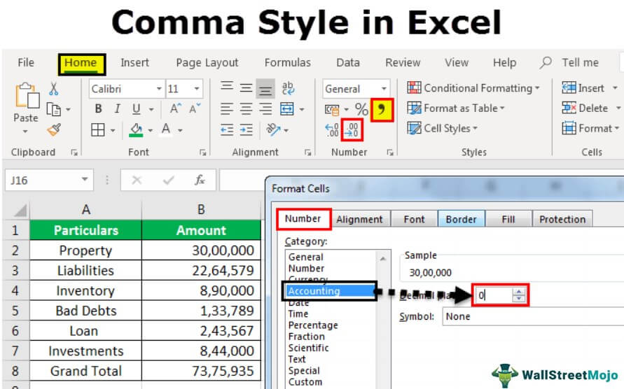
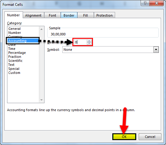
Then, we must select cells under the Amount column. Then, right-click on it, and choose Format Cells. After that, select the Accounting option under the Format Cells. If we do not want the decimal places, we can insert 0 under decimal places. And click on OK.
Below is the formatted data after removing decimal points.
Excel Shortcuts to Use Comma Style Format
- We must select the cells which need to format.

- Press the Alt key that enables the commands on the ExcelCommands On The ExcelVLOOKUP function, IF condition, CONCATENATE function, find MAXIMUM and MINIMUM values are the most commonly used excel commands.read more ribbon.

- Press H to select the Home tab in the Excel ribbonExcel RibbonThe ribbon is an element of the UI (User Interface) which is seen as a strip that consists of buttons or tabs; it is available at the top of the excel sheet. This option was first introduced in the Microsoft Excel 2007.read more , it enables the Home tab of Excel.
- Press 9 to decrease the decimal, and press 0 to increase the decimal point from values.
- If you want to open the format cells dialogue, press Ctrl+1.
- If you want to show a monetary valueMonetary ValueMonetary value refers to the value of a product or service measured in terms of money.read more without a currency symbol, you can click None under option format cells.
- Like the “Currency” format, the “Accounting” group is utilized for financial qualities. In any case, this arrangement adjusts the decimal purposes of numbers in a section. Likewise, the “Accounting” design shows zeros as dashes and negative numbers in brackets. Like the “Currency” format organizes, we can determine what number of decimal spots we need and whether to utilize a thousand separators. We cannot change the default show of negative numbers except if we make a custom number organization.

Advantages
- It helps to format the number when we are dealing with currency.
- It provides help in showing the correct value with commas.
- It is just a one step process.
- It is very easy and convenient to use.
Disadvantages
- It always enables the number format with a thousand separators.
- It provides the decimal points of two places while using this function.
Things to Remember
- Rather than choosing a range of cells, we can likewise tap on the letter over a column to select the whole column or the number next to a column to select an entire row. We can likewise tap the little box to one side of “A” or above “1” to choose the whole spreadsheet at once.
- We must always check and remove it if we do not need a comma.
- Decimal is also the user’s choice if they want to put a decimal in values or not.
- A custom Excel number format changes just the visual representation. For example, how value is shown in a cell. The basic value put away in a cell is not changed.
- The comma Excel format is a default option to show numbers with a comma in the thousands place and includes two decimal places (Eg: “13000” becomes “13,000.00). It may also enable us to change the visible cell styles in an area of the ribbon to easily select different options for comma and display format as required in our sheet.
Recommended Articles
This article is a guide to Comma Style in Excel. We discuss Comma Style in Excel format with shortcut keys, Excel examples, and a downloadable Excel template. You may learn more about Excel from the following articles: –
Источник

Excel Comma Style (Table of Contents)
- Comma Style in Excel
- How to Apply Comma Style in Excel?
Comma Style in Excel
Comma style is Excel mainly used for numbers to distinguish the different lengths like hundreds, thousands, millions, etc. This allows users to read and spell the numbers incorrect form. To enable the comma in any cell, select Format Cells from the right-click menu and, from the Number section, check the box of Use 1000 separator (,). We can also use the Home menu ribbons’ Commas Style under the number section. We can also even use short cut keys by pressing ALT + H + K simultaneously to apply comma style.
Comma style format is categorized under the Number format section in the Home tab.
Comma style format is also referred to as thousands separator.
This format will be very helpful when you are working on a large table of financial sales data (Quarterly or half or Annual sales data), Comma style format is applied here, and numbers appear better. It is used to define the behavior of digits in relation to the thousands or lacks or millions or billions of digits. Comma Style format offers a good alternative to the Currency format. Comma style format inserts commas in larger numbers to separate thousands, hundred thousand, millions, billions, and so on.
Comma style is a type of number format where it adds commas to large numbers, adds two decimal places (i.e. 1000 becomes 1,000.00), displays negative values in closed parentheses & represents zeros with a dash (–).
The shortcut key for comma style is ALT + HK.

Prior to working on comma style number format, we need to check whether decimal & thousand separators are enabled or not in excel. If it is not enabled, we need to enable it & update it by the below-mentioned steps.
- To check decimal and thousands of separators in Excel, click the File tab.
- Click Options in the list of items on the left-hand side, Excel Options dialog box appears.
- In the Excel Options dialog box. Click Advanced in the list of items on the left-hand side.
- Under the editing options, Click or Tick on the Use system separators checkbox if there is no checkmark in the box. The Decimal separator and Thousands separator edit boxes displayed once you click on the “Use system separators” checkbox. Here I selected a comma as the thousands separator and a full point as the decimal separator. After that, click on OK.
These separators are automatically inserted into all the numbers in your workbook when you use the comma style number format.
Different types of Numeric value or Number types that you come across in sales data are as follows.
- Positive
- Negative
- Zero
- Text
How to Apply Comma Style in Excel?
Let’s check out how comma style number format works on different types of Numeric value or Number types in Excel.
You can download this Comma Style Excel Template here – Comma Style Excel Template
Comma Style in Excel – Example # 1
In the below-mentioned example, I have monthly sales data of a company, which contains retail, online & vendor sales numbers on a monthly basis; in this raw sales data, the appearance of the data is without any number format applied to it.
So, I need to apply the comma style number format for these positive sales values.
To display sales numbers with comma style format in Excel:
- Select the cells containing numeric sales values for which I want to display numbers with comma style number format.
- On the Home tab, you can select the Comma symbol & click on the Comma Style .command in the Number group.
; after
Once you have clicked on the Comma Style button, you can see the changes in the sales value, where excel separates the thousands with a comma and adds two decimal places at the end.
In the first cell, you can observe where 7889 becomes 7,889.00. The result is shown below.
Comma Style in Excel – Example # 2
In the below-mentioned example, I have monthly sales data of a company, which contains retail, online & vendor sales numbers on a monthly basis, in this raw sales data, it contains both positive & negative values. Currently, the appearance of the sales data is without any number format applied to it.
So, I need to apply comma style number format for these positive & negative values.
To display numbers with comma style format in Excel:
- Select the cells containing numeric sales values for which I want to display numbers with comma style number format. On the Home tab, you can select the comma symbol & click on the Comma Style command in the Number group.
- Once you have clicked on the Comma Style button, you can see the changes in the sales value.
Where excel separates the thousands with a comma and adds two decimal places at the end, and it encloses negative sales values in a closed pair of parentheses.
Comma Style in Excel – Example # 3
In the below-mentioned example, I have monthly sales data of a company, which contains retail, online & vendor sales numbers on a monthly basis, in this raw sales data, it contains both positive & Zero values. Currently, the appearance of the sales data is without any number format applied to it.
So, I need to apply a comma style number format for these positive & Zero values.
To display numbers with comma style format in Excel:
- Select the cells containing numeric sales values for which I want to display numbers with comma style number format. On the Home tab, you can select the comma symbol & click on the Comma Style command in the Number group.
Once you have clicked on the Comma Style button, you can see the changes in the sales value.
Where excel separates the thousands with a comma and adds two decimal places at the end, and a dash symbol represents zero values.
Things to Remember
- The comma style number Format option in excel makes your data easier to access & readable; it also helps you to set up your sales data at an industry standard.
- Apart from various number format options in excel, you can create your own custom number format in Excel based on your choice.
Recommended Articles
This has been a guide to Comma Style in Excel. Here we discussed How to apply Comma Style in Excel along with practical examples and a downloadable excel template. You can also go through our other suggested articles –
- Excel Date Format
- Excel Data Formatting
- Merge Cells in Excel
- Wrap Text in Excel
Comma Style Formatting in Excel
The comma style is a formatting style used in visualizing numbers with commas when the values are over 1,000. Such as, if we use this style on data with a value of 100,000, then the result displayed will be as (100,000). This formatting style can be accessed from the “Home” tab in the number section and click on the 1,000 (,) separator, known as the comma style in Excel.
For example, we have a company’s monthly sales and production dataset without a number format. In such cases, if we need to apply the comma style number format for the positive values, comma style formatting in Excel separates the thousands with a comma. It adds two decimal places at the end and a dash symbol at the zero values. It can also help create the custom number format of our choice. Moreover, it also makes it easier to access and increases readability by setting up data at an industry standard.
The comma style format (also known as the thousands separator) regularly goes with the “Accounting” format. Like the “Accounting” position, the comma arrangement embeds commas in bigger numbers to isolate thousands, hundred thousand, millions, and all values considered.
The standard comma style format contains up to two decimal points and a thousand separators and locks the dollar sign to the extreme left half of the cell. Negative numbers are shown in enclosures. To apply this format in a spreadsheet, we must feature every cell and click “Comma Style Format” under formatting choices in ExcelFormatting is a useful feature in Excel that allows you to change the appearance of the data in a worksheet. Formatting can be done in a variety of ways. For example, we can use the styles and format tab on the home tab to change the font of a cell or a table.read more.
- Comma Style Formatting in Excel
- How to Apply Comma Style in Excel (accounting format)?
- Excel Shortcuts to Use Comma Style Format
- Advantages
- Disadvantages
- Things to Remember
- Recommended Articles
You are free to use this image on your website, templates, etc, Please provide us with an attribution linkArticle Link to be Hyperlinked
For eg:
Source: Comma Style in Excel (wallstreetmojo.com)
How to Apply Comma Style in Excel (accounting format)?
You can download this Comma Style Excel Template here – Comma Style Excel Template
Lets us start the below steps.
- We must first enter the values in Excel to use the comma number format in Excel.

- We can use accounting Excel format in the Number format ribbon, select the amount cell, click on ribbon home, and select the Comma Style from the Number format column.

- Once we click on the Comma Style, it will provide the comma-separated format value.

- If we want to remove the decimal, we must click on the icon under Number on Decrease Decimal.

- Once we remove the decimal, we can see below the value without decimals.

- Then, we must select cells under the Amount column. Then, right-click on it, and choose Format Cells. After that, select the Accounting option under the Format Cells. If we do not want the decimal places, we can insert 0 under decimal places. And click on OK.

- Below is the formatted data after removing decimal points.
Excel Shortcuts to Use Comma Style Format
- We must select the cells which need to format.
- Press the Alt key that enables the commands on the ExcelVLOOKUP function, IF condition, CONCATENATE function, find MAXIMUM and MINIMUM values are the most commonly used excel commands.read more ribbon.
- Press H to select the Home tab in the Excel ribbonThe ribbon is an element of the UI (User Interface) which is seen as a strip that consists of buttons or tabs; it is available at the top of the excel sheet. This option was first introduced in the Microsoft Excel 2007.read more, it enables the Home tab of Excel.
- Press 9 to decrease the decimal, and press 0 to increase the decimal point from values.
- If you want to open the format cells dialogue, press Ctrl+1.
- If you want to show a monetary valueMonetary value refers to the value of a product or service measured in terms of money. read more without a currency symbol, you can click None under option format cells.
- Like the “Currency” format, the “Accounting” group is utilized for financial qualities. In any case, this arrangement adjusts the decimal purposes of numbers in a section. Likewise, the “Accounting” design shows zeros as dashes and negative numbers in brackets. Like the “Currency” format organizes, we can determine what number of decimal spots we need and whether to utilize a thousand separators. We cannot change the default show of negative numbers except if we make a custom number organization.
Advantages
- It helps to format the number when we are dealing with currency.
- It provides help in showing the correct value with commas.
- It is just a one step process.
- It is very easy and convenient to use.
Disadvantages
- It always enables the number format with a thousand separators.
- It provides the decimal points of two places while using this function.
Things to Remember
- Rather than choosing a range of cells, we can likewise tap on the letter over a column to select the whole column or the number next to a column to select an entire row. We can likewise tap the little box to one side of “A” or above “1” to choose the whole spreadsheet at once.
- We must always check and remove it if we do not need a comma.
- Decimal is also the user’s choice if they want to put a decimal in values or not.
- A custom Excel number format changes just the visual representation. For example, how value is shown in a cell. The basic value put away in a cell is not changed.
- The comma Excel format is a default option to show numbers with a comma in the thousands place and includes two decimal places (Eg: “13000” becomes “13,000.00). It may also enable us to change the visible cell styles in an area of the ribbon to easily select different options for comma and display format as required in our sheet.
Recommended Articles
This article is a guide to Comma Style in Excel. We discuss Comma Style in Excel format with shortcut keys, Excel examples, and a downloadable Excel template. You may learn more about Excel from the following articles: –
- How to Use Find and Select in Excel?
- Subscript Excel
- Superscript Excel
- Format Phone Numbers in ExcelYou can format the phone numbers in excel for the selected cells with the help of the «format cells» option that appears on right-clicking. It doesn’t change the phone number credentials but standardizes its presentation on the sheet.read more
Reader Interactions
CSV – популярное расширение файлов, которые используются, в основном, для обмена данными между различными компьютерными программами. Чаще всего необходимости в открытии и редактировании таких документов нет. Однако в некоторых случаях перед пользователями может встать такая задача. Программа Excel позволяет это сделать, но в отличие от стандартных файлов в формате XLS и XLSX, простое открытие документа двойным щелчком мыши не всегда дает качественный результат, что может выражаться в некорректном отображении информации. Давайте посмотрим, каким образом можно открыть файлы с расширением CSV в Экселе.
-
Открываем CSV-файлы
- Метод 1: двойным щелчком или через контекстное меню
-
Метод 2: применяем Мастер текстов
- Метод 3: через меню “Файл”
- Заключение
Для начала давайте разберемся, что из себя представляют документы в данном формате.
CSV – аббревиатура, которая расшифровывается как “Comma-Separated Values” (на русском языке означает “значения, разделенные запятыми”).
Как следует из названия, в таких документах используются разделители:
- запятая – в англоязычных версиях;
- точка с запятой – в русскоязычных версиях программы.
Во время открытия документа в Excel основная задача (проблема) заключается в выборе способа кодировки, примененного при сохранении файла. Если будет выбрана не та кодировка, скорее всего, пользователь увидит множество нечитаемых символов, и полезность информации будет сведена к минимуму. Помимо этого, ключевое значение имеет используемый разделитель. Например, если документ был сохранен в англоязычной версии, а затем его пытаются открыть в русскоязычной, скорее всего, качество отображаемой информации пострадает. Причина, как мы ранее отметили, заключается в том, что в разных версиях используются разные разделители. Давайте посмотрим, как избежать этих проблем и как правильно открывать файлы CSV.
Прежде, чем приступить к более сложным методам, давайте рассмотрим самый простой. Он применим только в тех случаях, когда файл был создан/сохранен и открывается в одной и той же версии программы, а значит, проблем с кодировкой и разделителями быть не должно. Здесь возможно два варианта, опишем их ниже.
Excel установлена как программа по умолчанию для открытия CSV-файлов
Если это так, открыть документ можно как и любой другой файл – достаточно просто дважды щелкнуть по нему.

Для открытия CSV-фалов назначена другая программа или не назначена вовсе
Алгоритм действия в таких ситуациях следующий (на примере Windows 10):
- Щелкаем правой кнопкой мыши по файлу и в открывшемся контекстном меню останавливаемся на команде “Открыть с помощью”.
- Во вспомогательном меню система может сразу предложить программу Excel. В этом случае кликаем по ней, в результате чего файл откроется (как и при двойном щелчке по нему). Если нужной нам программы нет в списке, кликаем по пункту “Выбрать другое приложение”.

- Появится окно, в котором мы можем выбрать программу (чтобы раскрыть весь список доступных вариантов, требуется нажать кнопку “Еще приложения”), с помощью которой требуется открыть документ. Ищем то, что нам нужно и жмем OK. Чтобы назначить Excel приложением по умолчанию для данного типа файлов, предварительно ставим соответствующую галочку.

- В некоторых случаях, когда и в этом окошке не удается найти Эксель, щелкаем по кнопке “Найти другое приложение на этом компьютере” в конце списка.
- На экране отобразится окно, в котором мы переходим к расположению программы на ПК, отмечаем исполняемый файл с расширением EXE и жмем кнопку “Открыть”.


Независимо от того, какой из описанных выше способов был выбран, результатом будет открытие CSV-файла. Как мы упомянули выше, корректно отображаться содержимое будет только при соответствии кодировки и разделителей.

В остальных случаях может показываться нечто подобное:

Поэтому описанный метод подходит не всегда, и мы переходим к следующим.
Метод 2: применяем Мастер текстов
Воспользуемся интегрированным в программу инструментом – Мастером текстов:
- Открыв программу и создав новый лист, чтобы получить доступ ко всем функциям и инструментам рабочей среды, переключаемся во вкладку “Данные”, где щелкаем по кнопке “Получение внешних данных”. Среди раскрывшихся вариантов выбираем “Из текста”.

- Откроется окно, в котором нам нужно перейти к расположению файла, который требуется импортировать. Отметив его жмем кнопку “Импорт”.

- Появится Мастер текстов. Проверяем, чтобы была выбрана опция “с разделителями” для параметра “Формат данных”. Выбор формата зависит от кодировки, которая была использована при его сохранении. Среди самых популярных форматов можно отметить “Кириллицу (DOS)” и “Юникод (UTF-8)”. Понять, что сделан правильный выбор можно, ориентируясь на предварительный просмотр содержимого в нижней части окна. В нашем случае подходит “Юникод (UTF-8)”. Остальные параметры чаще всего не требует настройки, поэтому жмем копку “Далее”.

- Следующим шагом определяемся с символом, который служит в качестве разделителя. Так как наш документ был создан/сохранен в русскоязычной версии программы, выбираем “точку с запятой”. Здесь у нас, как и в случае с выбором кодировки, есть возможность попробовать различные варианты, оценивая результат в области предпросмотра (можно, в том числе, указать свой собственный символ, выбрав опцию “другой”). Задав требуемые настройки снова нажимаем кнопку “Далее”.
- В последнем окне, чаще всего, вносить какие-либо изменения в стандартные настройки не нужно. Но если требуется изменить формат какого-то столбца, сначала кликаем по нему в нижней части окна (поле “Образец”), после чего выбираем подходящий вариант. По готовности жмем “Готово”.
- Появится окошко, в котором выбираем способ импорта данных (на имеющемся или на новом листе) и жмем OK.
- Все готово, нам удалось импортировать данные CSV-файла. В отличие от первого метода, мы можем заметить, что была соблюдена ширина столбцов с учетом содержимого ячеек.


И последний метод, которым можно воспользоваться заключается в следующем:
- Запустив программу выбираем пункт “Отрыть”.Если программа уже ранее была открыта и ведется работа на определенном листе, переходим в меню “Файл”.Щелкаем по команде “Открыть” в списк команд.
- Жмем кнопку “Обзор”, чтобы перейти к окну Проводника.
- Выбираем формат “Все файлы”, переходим к месту хранения нашего документа, отмечаем его и щелкаем кнопку “Открыть”.
- На экране появится уже знакомый нам Мастер импорта текстов. Далее руководствуемся шагами, описанными в Методе 2.
 Если программа уже ранее была открыта и ведется работа на определенном листе, переходим в меню “Файл”.
 Щелкаем по команде “Открыть” в списк команд.


Заключение
Таким образом, несмотря на кажущуюся сложность, программа Эксель вполне позволяет открывать и работать с файлами в формате CSV. Главное – определиться с методом реализации. Если при обычном открытии документа (двойным щелчком мыши или через контекстное меню) его содержимое содержит непонятные символы, можно воспользоваться Мастером текста, который позволяет выбрать подходящую кодировку и знак разделителя, что напрямую влияет на корректность отображаемой информации.
Text to Columns
- Highlight the column that contains your list.
- Go to Data > Text to Columns.
- Choose Delimited. Click Next.
- Choose Comma. Click Next.
- Choose General or Text, whichever you prefer.
- Leave Destination as is, or choose another column. Click Finish.
Contents
- 1 How do I separate a row in Excel with a comma?
- 2 How do I split one column into multiple columns in Excel?
- 3 How do I add comma separated values to a csv file?
- 4 Can I split a column in Excel?
- 5 How do I separate columns in Excel?
- 6 How do you convert a column to a comma separated list?
- 7 Is comma delimited the same as comma Separated?
- 8 How do you format a comma in Excel?
- 9 How do you split a column?
- 10 How do you split a column by space in Excel?
- 11 How do I split a column in sheets?
- 12 How do you separate data in Excel formula?
- 13 How do I separate text in Excel formula?
- 14 How do you use concatenate?
- 15 How do you paste comma Separated Values in sheets?
- 16 How do you split names in Excel?
- 17 How do you split Data in a spreadsheet?
- 18 How do I change data in Excel to comma separated text?
- 19 What is a comma separated list?
- 20 How do you convert a list to a comma separated string?
How do I separate a row in Excel with a comma?
In the Split Cells dialog box, select Split to Rows or Split to Columns in the Type section as you need. And in the Specify a separator section, select the Other option, enter the comma symbol into the textbox, and then click the OK button.
How do I split one column into multiple columns in Excel?
How to Split one Column into Multiple Columns
- Select the column that you want to split.
- From the Data ribbon, select “Text to Columns” (in the Data Tools group).
- Here you’ll see an option that allows you to set how you want the data in the selected cells to be delimited.
- Click Next.
How do I add comma separated values to a csv file?
Since CSV files use the comma character “,” to separate columns, values that contain commas must be handled as a special case. These fields are wrapped within double quotation marks. The first double quote signifies the beginning of the column data, and the last double quote marks the end.
Can I split a column in Excel?
Split the content from one cell into two or more cells
Note: Excel for the web doesn’t have the Text to Columns Wizard. Instead, you can Split text into different columns with functions.On the Data tab, in the Data Tools group, click Text to Columns. The Convert Text to Columns Wizard opens.
How do I separate columns in Excel?
In the table, click the cell that you want to split. Click the Layout tab. In the Merge group, click Split Cells. In the Split Cells dialog, select the number of columns and rows that you want and then click OK.
How do you convert a column to a comma separated list?
How to convert an Excel column into a comma separated list?
- Open your excel sheet and select the cells of the column that you want to process.
- Now open word document, right click on it and from the context menu, select ‘Paste Options’ as ‘Keep texts only’.
- Now press ‘CTRL + H’ to open the ‘Find and Replace’ dialog.
Is comma delimited the same as comma Separated?
A comma delimited file is one where each value in the file is separated by a comma. Also known as a Comma Separated Value file, a comma delimited file is a standard file type that a number of different data-manipulation programs can read and understand, including Microsoft Excel.
How do you format a comma in Excel?
To enable the comma in any cell, select Format Cells from the right-click menu and, from the Number section, check the box of Use 1000 separator (,). We can also use the Home menu ribbons’ Commas Style under the number section.
How do you split a column?
Try it!
- Select the cell or column that contains the text you want to split.
- Select Data > Text to Columns.
- In the Convert Text to Columns Wizard, select Delimited > Next.
- Select the Delimiters for your data.
- Select Next.
- Select the Destination in your worksheet which is where you want the split data to appear.
How do you split a column by space in Excel?
Click the “Data” tab in the ribbon, then look in the “Data Tools” group and click “Text to Columns.” The “Convert Text to Columns Wizard” will appear. In step 1 of the wizard, choose “Delimited” > Click [Next]. A delimiter is the symbol or space which separates the data you wish to split.
How do I split a column in sheets?
Split data into columns
- On your computer, open a spreadsheet in Google Sheets.
- At the top, click Data.
- To change which character Sheets uses to split the data, next to “Separator” click the dropdown menu.
- To fix how your columns spread out after you split your text, click the menu next to “Separator”
How do you separate data in Excel formula?
If you ever need to split data from one column in your Microsoft Excel worksheet into two or more columns, you can use the LEFT, MID and RIGHT Text functions.
To extract the Account Number using the MID function.
- Select cell C2 .
- Enter the formula: =MID(A2,5,3)
- Copy the formula down.
How do I separate text in Excel formula?
1st method
You can do so, click on the header ( A , B , C , etc.). Then click the little triangle and select “Insert 1 right”. Repeat to create a second free column. In the first free column, write =SPLIT(B1,”-“) , with B1 being the cell you want to split and – the character you want the cell to split on.
How do you use concatenate?
There are two ways to do this:
- Add double quotation marks with a space between them ” “. For example: =CONCATENATE(“Hello”, ” “, “World!”).
- Add a space after the Text argument. For example: =CONCATENATE(“Hello “, “World!”). The string “Hello ” has an extra space added.
How do you paste comma Separated Values in sheets?
3 Answers
- Open a spreadsheet in Google Sheets.
- Paste the data you want to split into columns.
- In the bottom right corner of your data, click the Paste icon.
- Click Split text to columns. Your data will split into different columns.
- To change the delimiter, in the separator box, click.
How do you split names in Excel?
How to Separate Names in Excel?
- Step 1: Select the “full name” column.
- Step 2: In the Data tab, click on the option “text to columns.
- Step 3: The box “convert text to columns wizard” opens.
- Step 4: Select the file type “delimited” and click on “next.”
How do you split Data in a spreadsheet?
Select the text or column, then click the Data menu and select Split text to columns…. Google Sheets will open a small menu beside your text where you can select to split by comma, space, semicolon, period, or custom character. Select the delimiter your text uses, and Google Sheets will automatically split your text.
How do I change data in Excel to comma separated text?
You can convert an Excel worksheet to a text file by using the Save As command.
- Go to File > Save As.
- Click Browse.
- In the Save As dialog box, under Save as type box, choose the text file format for the worksheet; for example, click Text (Tab delimited) or CSV (Comma delimited).
What is a comma separated list?
A comma-separated list is produced for a structure array when you access one field from multiple structure elements at a time. For instance if S is a 5-by-1 structure array then S.name is a five-element comma-separated list of the contents of the name field.
How do you convert a list to a comma separated string?
Approach: This can be achieved with the help of join() method of String as follows.
- Get the List of String.
- Form a comma separated String from the List of String using join() method by passing comma ‘, ‘ and the list as parameters.
- Print the String.
Home / Excel Basics / How to Apply Comma Style in Excel
The comma style in Excel is also known as the thousand separator format that converts the large number values with the commas inserted as separators to distinguish the number value length into thousands, hundred thousand, millions, and so on.
When the user applies the comma format, it also adds decimal values to the numbers. So, in short, it works similarly to an accounting system format but it does not add any currency symbol to the number which accounting system formatting does.
The comma style separator could show the number values separated into lakhs or in million formats depending upon the region and default currency format selected within your system, but you can change it from lakhs to million and vice versa.
Like India follows a number value accounting system in lakhs and USA follows in millions. We have quick and easy steps mentioned below for you to apply comma style in Excel.
Apply Comma Style Using the Home tab
- First, select the cells or range of cells or the entire column where to apply the comma style.

- After that, go to the “Home” tab and click on the comma (,) icon under the “Number” group on the ribbon.

- Once you click on the comma (,) icon, your selected range will get applied with comma separators in the number values.


To increase or remove the decimal values from the numbers, simply select the range and then click on the “Increase or Decrease decimal value” icon under the same “Number” group on the ribbon.

Apply Comma Style Using Format Cells Option
- First, select the cells or range of cells or the entire column where to apply the comma style.
- After that, right click on the mouse and select the “Format Cells” option from the drop-down list.

- Once you click on “Format Cells” you will get the “Format Cells” dialog box opened.
- Now, under the “Number” tab, select the “Number” option and then checkmark the “Use 1000 Separator” box.
- In the end, Click OK, and your selected range will get applied with comma separators in the number values.
- To remove the decimal values, enter zero (0) in the “Decimal places” field.


Change the Comma Style Separators from Lakhs to Million format
Sometimes, comma separators show numbers values separated in lakhs due to the default region and currency format of your system, but can change the currency format to millions format by following the below steps:
- First, go to your system “Control Panel” and click on the “Change date, time, or number formats” link under the “Clock and Region” or “Region and Language” option. (Option names could be different depending on the Windows version)

- After that, click on “Additional Settings” within the “Region” dialog box.

- Once you click on “Additional Settings”, you will get the “Customize Format” dialog box opened.
- Now, select the “Currency” header and then select the format to million style format of separator commas option in digit grouping.
- In the end, click Apply and then Ok within the “Customize Format” dialog box and then in the “Region” dialog box.

- Once you are done, close and open the Excel file again and apply comma style and you will get your selected range will get applied with comma separators in thousand, hundred thousand, and million to the number values.


Apply Comma Style Using Keyboard Shortcut
Select the entire column or the range where to apply comma style and then press the Alt+ H + K keys and you will get your selected range applied with comma separators.

Why does Excel expect commas or semicolons to separate the parameters in a formula? The answer can be found in this article.
Comma or semicolon ?
If you read this article, it’s because one day you noticed that the separator between the parameters in any function is the comma sign or the semicolon.
Sometimes the separator is a comma

Sometimes the separator is a semicolon

How and where to change this option?
Don’t waste your time to find this option in Excel! This option is not in Excel but in the local settings of Windows 😮😮😮
Windows settings
To switch between comma or semicolon as separator, follow the next steps
1. Open your Windows settings
![]()
2. Select the Time & Language menu

3. Then select Region & language > Additional date, time & regional settings

4. Click on Region > Change location

Shortcuts
You can open the same dialog box with the command line intl.cpl in the search bar of Windows 😉👍

Change your setting
When you select a country in the dropdown list, the default date and number settings are loaded.
US settings
As you can see in the picture, the list separator is a comma. Also the date format is M/d/yyyy (month, day, year)

Now, when you write a formula, the separator between each arguments is a comma. And for the date as well, automatically your dates will be written with the US date format.
And You don’t have to Restart Excel to apply the settings. The change is immediate 😎😃👍
France, Spanish settings
If you don’t mind, you can change the values of the country to load semi-colon as default list separator. It’s the case for France or Spain. But in that case, your dates will be displayed in French or Spanish

Comma Style in Excel: A Comprehensive Guide to Excel’s Number Formatting
Excel is an amazing tool that can help you manage data efficiently. With the help of Excel, you can easily analyze data, create graphs, and generate reports. However, to make the most out of this tool, you need to have a good understanding of its features and functionalities. One such feature is the Comma Style in Excel. In this article, we will take an in-depth look at what Comma Style in Excel is and how to use it.
What is Comma Style in Excel?
Comma Style is a number formatting option in Excel that adds a thousands separator (comma) to a number, making it easier to read and understand. This formatting option can be applied to any number, including decimals and negative numbers. The Comma Style is particularly useful when dealing with large numbers or financial data, where it can help to highlight significant digits and make the data easier to read and interpret.
How to Apply Comma Style in Excel
Applying Comma Style to a number in Excel is a simple process that can be done in a few steps. To apply the Comma Style to a single cell or range of cells, follow these steps:
- Select the cell or range of cells you want to format.
- Click on the “Home” tab in the Excel ribbon.
- In the “Number” group, click on the drop-down arrow next to the “Number Format” box.
- Select “Comma Style” from the list of options.
Alternatively, you can use the keyboard shortcut “Ctrl + Shift + 1” to apply Comma Style to the selected cell or range of cells.
Customizing Comma Style in Excel
Excel’s Comma Style formatting option is customizable, meaning you can change the appearance of the thousands separator to suit your needs. To customize the Comma Style, follow these steps:
- Select the cell or range of cells you want to format.
- Click on the “Home” tab in the Excel ribbon.
- In the “Number” group, click on the drop-down arrow next to the “Number Format” box.
- Select “More Number Formats” at the bottom of the list.
- In the “Format Cells” dialog box, select “Number” from the list of categories.
- Under “Symbol,” select the symbol you want to use as the thousands separator. You can choose from comma, period, space, or any other symbol.
- Click “OK” to apply the custom Comma Style to the selected cell or range of cells.
Advantages of Using Comma Style in Excel
Comma Style in Excel offers several advantages when working with data. Here are some of the most significant benefits:
1. Improved Readability
The Comma Style makes it easier to read and interpret large numbers by adding separators that group digits into sets of three. Also, this helps to distinguish between the various digits and makes it easier to count them accurately.
2. Consistent Formatting
By using Comma Style consistently throughout a spreadsheet, you can ensure that all numbers are presented in the same format. This can help to maintain consistency and avoid confusion when working with data.
3. Highlighting Significant Digits
When working with financial data, it is often useful to highlight significant digits. Comma Style can help to achieve this by emphasizing the digits to the left of the decimal point, making it easier to identify the most significant values.
4. Improved Data Analysis
Comma Style can also be helpful when conducting data analysis. By making the data easier to read and interpret, you can quickly spot trends and patterns that may be missed if the data is presented in a less readable format.
Tips and Tricks for Using Comma Style in Excel
Now that you know how to use Comma Style in Excel, here are some tips and tricks to help you make the most out of this feature:
-
Use Comma Style to Make Large Numbers Easier to Read
As mentioned earlier, the Comma Style in Excel is a great way to make large numbers easier to read. By using this formatting feature, you can quickly identify the number of thousands or millions a number represents, making it easier to understand and analyze data.
-
Customize the Comma Style to Suit Your Needs
Excel allows you to customize the Comma Style to suit your needs. For instance, if you want to use a period as a thousands separator instead of a comma, you can easily do so by selecting the “Symbol” option and choosing the period symbol.
-
Use Comma Style with Other Formatting Features
Comma Style in Excel can be used with other formatting features to create more complex and visually appealing spreadsheets. For instance, you can use Comma Style in combination with Conditional Formatting to highlight specific values in your data.
-
Use Comma Style with PivotTables
Excel can also be used with PivotTables to make data analysis easier. By using Comma Style in your PivotTable, you can quickly identify trends and patterns in your data.

I am studying at Middle East Technical University. I am interested in computer science, architecture, physics and philosophy.
Love,
Cansu
Tags: #ExcelCharts #ExcelDashboard #ExcelFormulas #ExcelFunctions #ExcelTemplates #ExcelTipsAndTricks #ExcelTutorials