
Excel for Microsoft 365 Excel 2021 Excel 2019 Excel 2016 Excel 2013 Excel 2010 Excel 2007 More…Less
Important:
-
When you break a link to the source workbook of an external reference, all formulas that use the value in the source workbook are converted to their current values. For example, if you break the link to the external reference =SUM([Budget.xls]Annual!C10:C25), the SUM formula is replaced by the calculated value—whatever that may be. Also, because this action cannot be undone, you may want to save a version of the destination workbook as a backup.
-
If you use an external data range, a parameter in the query may be using data from another workbook. You may want to check for and remove any of these type of links.
Break a link
-
On the Data tab, in the Connections group, click Edit Links.

Note: The Edit Links command is unavailable if your file does not contain linked information.
-
In the Source list, click the link that you want to break.
-
To select multiple linked objects, hold down the CTRL key, and click each linked object.
-
To select all links, press Ctrl+A.
-
-
Click Break Link.
Delete the name of a defined link
If the link used a defined name, the name is not automatically removed. You may want to delete the name as well, by following these steps:
-
On the Formulas tab, in the Defined Names group, click Name Manager.
-
In the Name Manager dialog box, click the name that you want to change.
-
Click the name to select it.
-
Click Delete.
-
Click OK.
Need more help?
You can always ask an expert in the Excel Tech Community or get support in the Answers community.
Need more help?
![]()
Download Article
![]()
Download Article
If you’ve linked data from other worksheets in the same project or other spreadsheets in different file, but have since changed that information, this wikiHow will teach you how to break those links in Excel using a desktop computer. Which is useful if you’ve added links that you no longer want to keep active.
Steps
-
1
Open your document in Excel. You can either open your project within Excel by going to File > Open or you can right-click the Excel file in your file browser.
- This method works for Excel for Microsoft 365 and Excel 2019-2007 (Mac and Windows).
-
2
Click the Data tab. You’ll see this above the document editing space with Home, Formulas, and View.
Advertisement
-
3
Click Edit Links. You’ll find this in the «Queries & Connections» grouping.
- If you don’t see this button, the Excel sheet you’re working on does not have any active links.
-
4
Click the link you want to break. You’ll see a list of links that are active in your spreadsheet, single-clicking one will highlight it.
- If you want to select more than one link from the list, hold the CTRL (Windows) or CMD (Mac) key.
- If you want to select all the links, press CTRL + A (Windows) or CMD + A (Mac).
-
5
Click Break Link. You’ll need to confirm that you want to break the link to continue.[1]


Advertisement
Ask a Question
200 characters left
Include your email address to get a message when this question is answered.
Submit
Advertisement
Thanks for submitting a tip for review!
References
About This Article
Article SummaryX
1. Open your document in Excel.
2. Click the Data tab.
3. Click Edit Links.
4. Click the link you want to break.
5. Click Break Link.
Did this summary help you?
Thanks to all authors for creating a page that has been read 17,553 times.
Is this article up to date?
Хитрости »
30 Декабрь 2018 78855 просмотров
Невозможно разорвать связи с другой книгой
Прежде чем разобрать причины ошибки разрыва связей, не лишним будет разобраться что такое вообще связи в Excel и откуда они берутся. Если все это Вам известно — можете пропустить этот раздел 
- Что такое связи в Excel и как их создать
- Как разорвать/удалить связи
- Что делать, если связи не разрываются
Иногда при работе с различными отчетами приходится создавать связи с другими книгами(отчетами). Чаще всего это используется в функциях вроде ВПР(VLOOKUP) для получения данных по критерию из таблицы, расположенной в другой книге. Так же это может быть и простая ссылка на ячейки другой книги. В итоге ссылки в таких ячейках выглядят следующим образом:
=ВПР(A2;'[Продажи 2018.xlsx]Отчет’!$A:$F;4;0)
или
='[Продажи 2018.xlsx]Отчет’!$A1
- [Продажи 2018.xlsx] — обозначает книгу, в которой итоговое значение. Такие книги так же называют источниками
- Отчет — имя листа в этой книге
- $A:$F и $A1 — непосредственно ячейка или диапазон со значениями
Если закрыть книгу, на которую была создана такая ссылка, то ссылка сразу изменяется и принимает более «длинный» вид:
=ВПР(A2;’C:UsersДмитрийDesktop[Продажи 2018.xlsx]Отчет’!$A:$F;4;0)
=’C:UsersДмитрийDesktop[Продажи 2018.xlsx]Отчет’!$A1
Предположу, что большинство такими ссылками не удивишь. Такие ссылки так же принято называть связыванием книг. Поэтому как только создается такая ссылка на вкладке Данные(Data) в группе Запросы и подключения(Queries & Coonections) активируется кнопка Изменить связи(Edit Links). Там же, как несложно догадаться, их можно изменить. В большинстве случаев ни использование связей, ни их изменение не доставляет особых проблем. Даже если в книге источники были изменены значения ячеек, то при открытии книги со связью эти изменения будут так же автоматом обновлены. Но если книгу-источник переместили или переименовали — при следующем открытии книги со ссылками на неё Excel покажет сообщение о недоступных связях в книге и запрос на обновление этих ссылок:

Если нажать Продолжить, то ссылки обновлены не будут и в ячейках будут оставлены значения на момент последнего сохранения. Происходит это потому, что ссылки хранятся внутри самой книги и так же там хранятся значения этих ссылок. Если же нажать Изменить связи(Change Source), то появится окно изменения связей, где можно будет выбрать каждую связь и указать правильное расположение нужного файла:

Так же изменение связей доступно непосредственно из вкладки Данные(Data)
Как разорвать связи
Как правило связи редко нужны на продолжительное время, т.к. они неизбежно увеличивают размер файла, особенно, если связей много. Поэтому чаще всего связь создается только для единовременно получения данных из другой книги. Исключениями являются случаи, когда связи делаются на общий файл, который ежедневного изменяется и дополняется различными сотрудниками и подразделениями, а в итоговом файле необходимо использовать именно актуальные данные этого файла.
Если решили разорвать связь, необходимо перейти на вкладку
Данные(Data)
-группа
Запросы и подключения(Queries & Coonections)
—
Изменить связи(Edit Links)
:
Выделить нужные связи и нажать
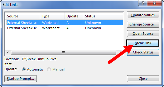
Разорвать связь(Break Link)
. При этом все ячейки с формулами, содержащими связи, будут преобразованы в значения вычисленные этой формулой при последнем обновлении. Данное действие нельзя будет отменить — только закрытием книги без сохранения.
Так же связи внутри формул разрываются, если формулы просто заменить значениями -выделяем нужные ячейки -копируем их -не снимая выделения жмем
Правую кнопку мыши
—
Специальная вставка(Paste Special)
—
Значения(Values)
. Формулы в ячейках будут заменены результатами их вычислений, а все связи будут удалены.
Более подробно про замену формул значениями можно узнать из статьи: Как удалить в ячейке формулу, оставив значения?
Что делать, если связи не разрываются
Но иногда возникают ситуации, когда вроде все формулы во всех ячейках уже заменены на значения, но запрос на обновление каких-то связей все равно появляется. В этом случае есть парочка рекомендаций для поиска и удаления этих мифических связей:
- проверьте нет ли каких-либо связей в именованных диапазонах:
нажмите сочетание клавиш Ctrl+F3 или перейдите на вкладку Формулы(Formulas) —Диспетчер имен(Name Manager)
Читать подробнее про именованные диапазоны
Если в каком-либо имени есть ссылка с полным путем к какой-то книге(вроде такого ‘[Продажи 2018.xlsx]Отчет’!$A1), то такое имя надо либо изменить, либо удалить. Кстати, некоторые имена в итоге могут выдавать ошибку #ССЫЛКА!(#REF!) — к ним тоже стоит присмотреться. Имена с ошибками ничего хорошего как правило не делают.
Настоятельно рекомендую перед удалением имен создать резервную копию файла, т.к. неверное удаление таких имен может повлечь неправильную работу файла даже в случае, если сами ссылки возвращали в итоге ошибочное значение. - если удаление лишних имен не дает эффекта — проверьте условное форматирование:
вкладка Главная(Home) —Условное форматирование(Conditional formatting) —Управление правилами(Manage Rules). В выпадающем списке проверить каждый лист и условия в нем:

Может случиться так, что условие было создано с использованием ссылки на другие книги. Как правило Excel запрещает это делать, но если ссылка будет внутри какого-то именованного диапазона — то диапазон такой можно будет применить в УФ, но после его удаления в самом УФ это имя все равно остается и генерирует ссылку на файл-источник. Такие условия можно удалять без сомнений — они все равно уже не выполняются как положено и лишь создают «пустую» связь. - Так же не помешает проверить наличие лишних ссылок и среди проверки данных(Что такое проверка данных). Как правило связи могут быть в проверке данных с типом Список. Но как их отыскать, если проверка данных распространена на множество ячеек?
Находим все ячейки с проверкой данных: выделяем одну любую ячейку на листе -вкладка Главная(Home) -группа Редактирование(Editing) —Найти и выделить(Find & Select) —Выделить группу ячеек(Go to Special). Отмечаем Проверка данных(Data validation) —Всех(All). Жмем Ок. После этого можно выделить все эти ячейки каким-либо цветом, чтобы удобнее было потом просматривать. Но такой метод выделит ВСЕ ячейки с проверками данных, а не только ошибочные.
Конечно, если вариантов кроме как найти руками нет и ячеек немного – просто заходим в проверку данных каждой ячейки(выделяем эту ячейку -вкладка Данные(Data) —Проверка данных(Data validation)) и смотрим, есть ли там проблемная формула со ссылками на другие книги.
Можно поступить более кардинально – после того как выделили все ячейки с проверкой данных идем на вкладку Данные(Data) —Проверка данных(Data validation) и для всех ячеек в поле Тип данных(Allow) выбираем Любое значение(Any value). Это удалит все формулы из проверки данных всех ячеек.
Но если ни удаление всех проверок данных, ни проверка каждой ячейки не подходит — я предлагаю коротенький код, который отыщет все такие ссылки быстрее и сэкономит время:Option Explicit '--------------------------------------------------------------------------------------- ' Author : The_Prist(Щербаков Дмитрий) ' Профессиональная разработка приложений для MS Office любой сложности ' Проведение тренингов по MS Excel ' https://www.excel-vba.ru ' info@excel-vba.ru ' WebMoney - R298726502453; Яндекс.Деньги - 41001332272872 ' Purpose: '--------------------------------------------------------------------------------------- Sub FindErrLink() 'надо посмотреть в Данные -Изменить связи ссылку на файл-иточник 'и записать сюда ключевые слова в нижнем регистре(часть имени файла) 'звездочка просто заменяет любое кол-во символов, чтобы не париться с точным названием Const sToFndLink$ = "*продажи 2018*" Dim rr As Range, rc As Range, rres As Range, s$ 'определяем все ячейки с проверкой данных On Error Resume Next Set rr = ActiveSheet.UsedRange.SpecialCells(xlCellTypeAllValidation) If rr Is Nothing Then MsgBox "На активном листе нет ячеек с проверкой данных", vbInformation, "www.excel-vba.ru" Exit Sub End If On Error GoTo 0 'проверяем каждую ячейку на предмет наличия связей For Each rc In rr 'на всякий случай пропускаем ошибки - такое тоже может быть 'но наши связи должны быть без них и они точно отыщутся s = "" On Error Resume Next s = rc.Validation.Formula1 On Error GoTo 0 'нашли - собираем все в отдельный диапазон If LCase(s) Like sToFndLink Then If rres Is Nothing Then Set rres = rc Else Set rres = Union(rc, rres) End If End If Next 'если связь есть - выделяем все ячейки с такими проверками данных If Not rres Is Nothing Then rres.Select ' rres.Interior.Color = vbRed 'если надо выделить еще и цветом End If End Sub
Чтобы правильно использовать приведенный код, необходимо скопировать текст кода выше, перейти в редактор VBA(Alt+F11) -создать стандартный модуль(Insert —Module) и в него вставить скопированный текст. После чего вызвать макросы(Alt+F8 или вкладка Разработчик —Макросы), выбрать FindErrLink и нажать выполнить.
Есть пара нюансов:- Прежде чем искать ненужную связь необходимо определить её ссылку: Данные(Data) -группа Запросы и подключения(Queries & Coonections) —Изменить связи(Edit Links). Запомнить имя файла и записать в этой строке внутри кавычек:
Const sToFndLink$ = «*продажи 2018*»
Имя файла можно записать не полностью, все пробелы и другие символы можно заменить звездочкой дабы не ошибиться. Текст внутри кавычек должен быть в нижнем регистре. Например, на картинках выше есть связь с файлом «Продажи 2018.xlsx», но я внутри кода записал «*продажи 2018*» — будет найдена любая связь, в имени которой есть «продажи 2018». - Код ищет проверки данных только на активном листе
- Код только выделяет все найденные ячейки(обычное выделение), он ничего сам не удаляет
- Если надо подсветить ячейки цветом — достаточно убрать апостроф(‘) перед строкой
rres.Interior.Color = vbRed ‘если надо выделить еще и цветом
- Прежде чем искать ненужную связь необходимо определить её ссылку: Данные(Data) -группа Запросы и подключения(Queries & Coonections) —Изменить связи(Edit Links). Запомнить имя файла и записать в этой строке внутри кавычек:

Как правило после описанных выше действий лишних связей остаться не должно. Но если вдруг связи остались и найти Вы их никак не можете или по каким-то причинам разорвать связи не получается(например, лист со связью защищен)- можно пойти совершенно иным путем. Действует этот рецепт только для файлов новых форматов Excel 2007 и выше (если проблема с файлом более старого формата — можно пересохранить в новый формат):
- Обязательно делаем резервную копию файла, связи в котором никак не хотят разрываться
- Открываем файл при помощи любого архиватора(WinRAR отлично справляется, но это может быть и другой, работающий с форматом ZIP)
- В архиве перейти в папку xl -> externalLinks
- Сколько связей содержится в файле, столько файлов вида externalLink1.xml и будет внутри. Файлы просто пронумерованы и никаких сведений о том, к какому конкретному файлу относится эта связь на поверхности нет. Чтобы узнать какой файл .xml к какой связи относится надо зайти в папку «_rels» и открыть там каждый из имеющихся файлов вида externalLink1.xml.rels. Там и будет содержаться имя файла-источника.
- Если надо удалить только связь на конкретный файл — удаляем только те externalLink1.xml.rels и externalLink1.xml, которые относятся к нему. Если удалить надо все связи — удаляем все содержимое папки externalLinks
- Закрываем архив
- Открываем файл в Excel. Появится сообщение об ошибке вроде «Ошибка в части содержимого в Книге …». Соглашаемся. Появится еще одно окно с перечислением ошибочного содержимого. Нажимаем закрыть.
После этого связи должны быть удалены.
Если и это не помогло — скорее всего «битая» связь связана с ошибкой самого файла и лучшим решением будет перенести все данные в новый файл.
Так же см.:
Найти скрытые связи
Оптимизировать книгу
Статья помогла? Поделись ссылкой с друзьями!
![]() Видеоуроки
Видеоуроки
Поиск по меткам
Access
apple watch
Multex
Power Query и Power BI
VBA управление кодами
Бесплатные надстройки
Дата и время
Записки
ИП
Надстройки
Печать
Политика Конфиденциальности
Почта
Программы
Работа с приложениями
Разработка приложений
Росстат
Тренинги и вебинары
Финансовые
Форматирование
Функции Excel
акции MulTEx
ссылки
статистика
Содержание
- Метод Workbook.BreakLink (Excel)
- Синтаксис
- Параметры
- Пример
- Поддержка и обратная связь
- Break a link to an external reference in Excel
- Break a link
- Delete the name of a defined link
- Need more help?
- Break a link to an external reference in Excel
- Break a link
- Delete the name of a defined link
- Need more help?
- Break Links in Excel
- How to Break External Links in Excel?
- 2 Different Methods to Break External Links in Excel
- Method #1 – Copy and Paste as Values
- Method #2 – Edit Options Tab
- Things to Remember
- Recommended Articles
- Break Links in Excel – All of Them (Even When Excel Doesn’t)
- Break ‘normal’ workbook links within formulas
- Break links from named ranges
- Break Data Validation links
- Break links of Conditional Formatting rules
- Break links of Pivot Tables
- Break all links with Professor Excel Tools
Метод Workbook.BreakLink (Excel)
Преобразует формулы, связанные с другими источниками Microsoft Excel или ole-источниками, в значения.
Синтаксис
expression. BreakLink (имя, тип)
Выражение Переменная, представляющая объект Workbook .
Параметры
| Имя | Обязательный или необязательный | Тип данных | Описание |
|---|---|---|---|
| Name | Обязательный | String | Имя ссылки. |
| Тип | Обязательный | XlLinkType | Тип ссылки. |
Пример
В этом примере Microsoft Excel преобразует первую ссылку (тип ссылки Excel) в активную книгу. В этом примере предполагается, что в активной книге существует по крайней мере одна формула, которая ссылается на другой источник Excel.
Поддержка и обратная связь
Есть вопросы или отзывы, касающиеся Office VBA или этой статьи? Руководство по другим способам получения поддержки и отправки отзывов см. в статье Поддержка Office VBA и обратная связь.
Источник
Break a link to an external reference in Excel
When you break a link to the source workbook of an external reference, all formulas that use the value in the source workbook are converted to their current values. For example, if you break the link to the external reference =SUM([Budget.xls]Annual!C10:C25), the SUM formula is replaced by the calculated value—whatever that may be. Also, because this action cannot be undone, you may want to save a version of the destination workbook as a backup.
If you use an external data range, a parameter in the query may be using data from another workbook. You may want to check for and remove any of these type of links.
Break a link
On the Data tab, in the Connections group, click Edit Links.

Note: The Edit Links command is unavailable if your file does not contain linked information.
In the Source list, click the link that you want to break.
To select multiple linked objects, hold down the CTRL key, and click each linked object.
To select all links, press Ctrl+A.
Click Break Link.
Delete the name of a defined link
If the link used a defined name, the name is not automatically removed. You may want to delete the name as well, by following these steps:
On the Formulas tab, in the Defined Names group, click Name Manager.
In the Name Manager dialog box, click the name that you want to change.
Click the name to select it.
Need more help?
You can always ask an expert in the Excel Tech Community or get support in the Answers community.
Источник
Break a link to an external reference in Excel
When you break a link to the source workbook of an external reference, all formulas that use the value in the source workbook are converted to their current values. For example, if you break the link to the external reference =SUM([Budget.xls]Annual!C10:C25), the SUM formula is replaced by the calculated value—whatever that may be. Also, because this action cannot be undone, you may want to save a version of the destination workbook as a backup.
If you use an external data range, a parameter in the query may be using data from another workbook. You may want to check for and remove any of these type of links.
Break a link
On the Data tab, in the Connections group, click Edit Links.
Note: The Edit Links command is unavailable if your file does not contain linked information.
In the Source list, click the link that you want to break.
To select multiple linked objects, hold down the CTRL key, and click each linked object.
To select all links, press Ctrl+A.
Click Break Link.
Delete the name of a defined link
If the link used a defined name, the name is not automatically removed. You may want to delete the name as well, by following these steps:
On the Formulas tab, in the Defined Names group, click Name Manager.
In the Name Manager dialog box, click the name that you want to change.
Click the name to select it.
Need more help?
You can always ask an expert in the Excel Tech Community or get support in the Answers community.
Источник
Break Links in Excel


How to Break External Links in Excel?
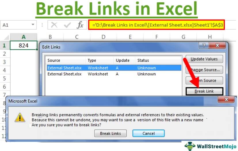
There are two different methods to break external links in the Excel worksheet. The first method is to copy and paste as a value method, which is very simple. The second method is a little different. First, we need to go to the “DATA” tab and click “Edit Links,” and find the option to break the link.
Table of contents
You are free to use this image on your website, templates, etc., Please provide us with an attribution link How to Provide Attribution? Article Link to be Hyperlinked
For eg:
Source: Break Links in Excel (wallstreetmojo.com)
2 Different Methods to Break External Links in Excel
Method #1 – Copy and Paste as Values
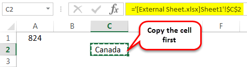
Now, we must paste them as values.
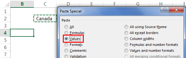
We can see here that this value does not contain any links. It shows only value.

Method #2 – Edit Options Tab
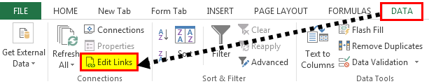
The second method is a little different. In this method, we must go to the “DATA” tab and click on “Edit Links.”
Now, we can see the below-shown dialogue box.
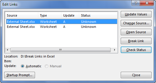
Here we can see all the available external links. We can update the values, open-source files, and many other things. Apart from all these, we can also break these links.
Now, we will click on the “Break Link.”
As soon as we click on “Break Link,” we may see the dialog box below.
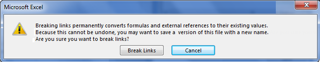
If we wish to break all the links at once, we need to select all the links and click on “Break Links.”
Things to Remember
- It is dangerous to have links to external sources in Excel.
- Once we break the link in Excel, we cannot undo the action.
- Using *.xl can cover all kinds of file extensions.
Recommended Articles
This article is a guide to Break Links in Excel. We discuss how to break external links in Excel using Copy and Paste as Value and Edit the Links Option tab, along with practical examples. You may learn more about Excel from the following articles: –
Источник
Break Links in Excel – All of Them (Even When Excel Doesn’t)

When you copy cells or worksheets from another Excel workbook, links to other worksheets in many cases still persists. Excel offers a function to break links but this function only works with links within formulas. There are many other types of links as links within conditional formatting rules or data validation rules. The bad news: Those links can’t be cut easily. The good news: there are still ways to break these links.
Break ‘normal’ workbook links within formulas
Usually, “normal” workbook links within formulas can be cut easily with the ‘Edit Links’ function included in Excel (the numbers are corresponding with the picture on the right hand side):
- Go to the Data ribbon.
- If the “Edit Links” button is not greyed out it means that there is at least one active link to another data source (usually another workbook). Click on that button.
- Select all the data links you’d like to kill.
- Click on Break Link.
Please be careful: all cells referring to other workbooks within formulas will be changed to values. The underlying formulas will be removed.
If you want to avoid that the formulas are removed you might want to try another (more manual) approach: Using the replace function in Excel to replace the links with nothing:
- Find a cell relating to another workbook within a formula.
- Copy the link, shown with the square brackets inside the formula.
- Make sure that the exact same sheet as the source sheet also exists in your current workbook.
- Press Ctrl + h for opening the replace dialogue box.
- Paste the copied link and leave the Replace field blank.
- Click on Find Next.
Break links from named ranges
You can name cells in Excel. Instead of the cell reference as “A1” just the cell name will be shown. Breaking such links is easy:
- On the Formulas ribbon go to Name Manager and you can see all the names in your workbook.
- Please check in the reference column whether a cell name refers to another workbook. Just delete the entry if you want to cut that link.
Break Data Validation links
If you have data validation rules in your workbook – such as dropdown lists within cells – it’s possible that they relate to other workbooks. Unless you know exactly which cells have such rules you unfortunately have to search them.
Once you found cells having data validation rules referring to other workbooks follow these steps:
- Select the cells having data validation rules referring to other workbooks.
- Go to the Data ribbon.
- Next, click on Data Validation.
- The most common is the type List. If the source refers to other workbooks you should remove the path and link them to a place within your workbook. Alternatively remove the data validation rule completely by setting the “Allowed” type to “Any Value”.
Do you want to boost your productivity in Excel?
Get the Professor Excel ribbon!

Add more than 120 great features to Excel!
Break links of Conditional Formatting rules
Conditional Formatting rules can relate to other workbook as well. Especially when copying worksheets to other workbooks such links can be created. Finding them must be done for each worksheet separately:
- Click on Conditional Formatting in the center of the Home ribbon.
- Click on Manage Rules.
- In the drop down list on the top of the newly opened window select ‘This Sheet’. Now all the conditional formatting rules of the current worksheet will be shown.
- The easiest way is deleting the rules referring to other workbooks. Otherwise you have to change them manually and link them to your current workbook.
Break links of Pivot Tables
If the data source of Pivot Tables is in another workbook you can break this link too. Therefore, follow these steps:
- Find out if the data source of your Pivot Table is located on another workbook as described in this article.
- If the Pivot Table links to another workbook you have two options:
- Set another data source within your current workbook.
- Remove the Pivot functionality and copy and paste the complete Pivot Table as values.
Because cutting links in Excel can be very troublesome and takes a lot of time, we’ve included a break link manager in our Excel add-in ‘Professor Excel Tools’. All the above mentioned steps are provided.
For breaking all the workbook links follow these steps:
- Go to the Professor Excel ribbon. and click on the ‘Break Link Manager’ within the ‘Workbook Tools’ group (the button with crossed out link on it). Professor Excel Tools now counts how many times each link type can be found within your Excel table.
- Select all the link types you’d like to break and click on start.
- Now, Professor Excel will break all the links. This procedure can take some time, especially if you have a lot of data in your workbook. The current status is shown in the status bar on the bottom of the screen.
Try it for free and see if it works for you.

This function is included in our Excel Add-In ‘Professor Excel Tools’
(No sign-up, download starts directly)
More than 35,000 users can’t be wrong.
Источник
How to Break External Links in Excel?
There are two different methods to break external links in the Excel worksheet. The first method is to copy and paste as a value method, which is very simple. The second method is a little different. First, we need to go to the “DATA” tab and click “Edit Links,” and find the option to break the link.
Table of contents
- How to Break External Links in Excel?
- 2 Different Methods to Break External Links in Excel
- Method #1 – Copy and Paste as Values
- Method #2 – Edit Options Tab
- Things to Remember
- Recommended Articles
- 2 Different Methods to Break External Links in Excel
You are free to use this image on your website, templates, etc, Please provide us with an attribution linkArticle Link to be Hyperlinked
For eg:
Source: Break Links in Excel (wallstreetmojo.com)
2 Different Methods to Break External Links in Excel
Method #1 – Copy and Paste as Values
Now, we must paste them as values.
We can see here that this value does not contain any links. It shows only value.
Method #2 – Edit Options Tab
The second method is a little different. In this method, we must go to the “DATA” tab and click on “Edit Links.”
Now, we can see the below-shown dialogue box.
Here we can see all the available external links. We can update the values, open-source files, and many other things. Apart from all these, we can also break these links.
Now, we will click on the “Break Link.”
As soon as we click on “Break Link,” we may see the dialog box below.
Once we break the External link in ExcelExternal links are also known as external references in Excel. When we use a formula in Excel and refer to a new workbook, it is the external link to the formula. In other words, an external link is when we give a link or apply a formula from another workbook.read more, we cannot recover the formulas. So, we cannot undo the action once we break the link. It is unlike our “Paste Special” method.
If we wish to break all the links at once, we need to select all the links and click on “Break Links.”
Things to Remember
- It is dangerous to have links to external sources in Excel.
- Once we break the link in Excel, we cannot undo the action.
- Using *.xl can cover all kinds of file extensions.
Recommended Articles
This article is a guide to Break Links in Excel. We discuss how to break external links in Excel using Copy and Paste as Value and Edit the Links Option tab, along with practical examples. You may learn more about Excel from the following articles: –
- Hyperlink Excel Formula
- VBA Hyperlinks
- How to Insert Hyperlinks in Excel?
- How to Remove Hyperlinks in Excel?
- Page Setup in Excel