Choose ms excel function to sum the numbers - Word и Excel - помощь в работе с программами

Download Article

Simple and advanced methods to sum in Excel

Download Article

Using the Plus Sign (+)

Using the SUM Function

Using the SUMIF Function

Using the SUMIFS Function

Tips

Whether you’re working with a few numbers or large datasets, there’s a Microsoft Excel summation formula for you! The most common adding function is “=SUM()”, with the target cell range placed between the parentheses. But, there are various ways to add numbers in your spreadsheet. This wikiHow guide will show you how to use summation formulas in Microsoft Excel. We’ll cover 4 methods: the plus sign operator (+), =SUM, =SUMIF, and =SUMIFS.

Things You Should Know

For small-scale addition, use “=cell1 + cell2 + cell3 + …” to sum cell values.
For larger sets of data, use “=SUM(your numbers here)” to sum a range of values
To add values if they meet one criterion, use “=SUMIF(range, criteria, [sum_range])” where sum_range is optional.
To add values if they meet multiple criteria, use “=SUMIFS(sum_range, criteria_range1, criteria1, [criteria_range2, criteria2], …)”.

Choose a Method

Plus sign: Simple and intuitive, but inefficient. Best for small, quick sums.
SUM function: Useful for large spreadsheets as it can sum a range of cells. Can only accept numeric arguments, not conditional values.
SUMIF function: Allows you to specify a condition, and only sum values that meet that condition.
SUMIFS function: Allows for complex logical statements by setting multiple criteria. Not available for Excel 2003 or earlier.

1
Enter the formula into a new cell. Make a new spreadsheet. Then, select a cell and type an equals sign (=). Then, alternate between clicking a cell with a value, and typing “+”. Your formula should end with the final cell you want to sum. Your finished formula should look like cell1 + cell2 + cell3. Hit the Enter key when you complete your formula.
- For example, =C4+C5+C6+C7 will sum the values of the four cells, C4, C5, C6, and C7.
- Each time you click on another cell, Excel will insert the cell reference for you (C4, for example), which tells Excel which spreadsheet cell contains the number (for C4, it’s the cell in column C, in row 4).
- If you know which cells you want to calculate, you can type them out instead of clicking them individually.
- Excel functions will recognize a combination of numbers and cell references in formulas. For example, you could type “=5000+C5+25.2+B7”.
- If you’re looking for subtraction information, check out our guide on how to subtract in Excel.

1
Use the SUM function to add two or more cells. Select the cell you want the summation to output to. Then, type an equals sign (=), SUM, and the cells you’re summing enclosed in parenthesis. The function should look like this: =SUM(your numbers here).
- For example, =SUM(C4,C5,C6,C7) will add the numbers contained in the 4 cells within the parentheses.
2
Use the SUM function to add a range of cells. If you provide a starting and ending cell, separated by a colon (:), you can sum large sections of the spreadsheet. The function should look like this: =SUM(cell1:cell2)’ where “cell1” and “cell2” are your starting and ending cell respectively.
- For example, =SUM(C4:C7) sums the values in C4 to C7.
- You don’t have to type out “C4:C7”. After typing “=SUM(” you can select a range by clicking and dragging your cursor from cell C4 to C7. The range will appear in the formula following the open parenthesis. Add the closing parenthesis at the end, and you’re done!
- For a large range of numbers, this is much faster than clicking on each cell individually.
3
Use the AutoSum Wizard. If you’re using Excel 2007 or later, an alternative to typing “=SUM” is using AutoSum.^[1]
- Select the cell you want the summation to output to.
- Go to the Format tab > AutoSum drop-down arrow > Sum.
- Select the range of cells you want to sum.
- AutoSum might be limited to contiguous cell ranges in some versions of Excel; if you want to skip cells in your calculation, it may not work correctly.
4
Copy/paste data into other cells. Since the cell with the function holds both the sum value and the sum function, you have to consider which you want copied.
- Copy the cell with the summation by pressing Ctrl + c (Windows) or Cmd + c (Mac). Then, select another cell and go to the Home tab > Clipboard drop-down and select either Paste Formulas or Paste Values.
5
Reference sums in other functions. You can use the value of your summation cell in other functions. Rather than making a new summation or typing out the number value of your previous function, you can reference the original sum cell in other calculations.
- For example, let’s say you create a summation function for column C in C20 and column D in D20. You can add these sums by selecting a new cell and typing “=SUM(C20, D20)”
- This essentially nests your two summations into a third summation formula. Then, if your summation of C or D changes, this third summation will automatically update.

1
Use the basic SUMIF function. The SUMIF function allows you to sum values when they meet a criteria. The criteria can be within the range of values itself, or in a different range that is the same size as the values range. If the criteria is in the range itself, follow these steps:^[2]
- Type =SUMIF( in a new cell.
- Select or type the range of cells you want to sum, then type a comma (,).
- Type a numerical criteria in double quotation marks, then type a closing parenthesis.
- For example, if you want to only sum numbers in a range that are greater than 10, you could type “=SUM(C1:C10, “>10”)”
2
Set up your data for SUMIF. If you’re using the optional parameter [sum_range], you’ll need separate columns for the range you want compared to the criteria and the range you want to sum. There are multiple ways to format a spreadsheet, but here’s a basic setup for SUMIF:
- Create one column with number values and a second column with a conditional value, like “yes” and “no”.
- For example, a column with 4 rows with values 1, 2, 3, and 4 and a second column with values of “yes” or “no”.
- This setup is similar to using VLOOKUP.
3
Enter the function into a cell. To create a SUMIF formula using the optional [sum_range], follow these steps:
- Select a new cell and enter “=SUMIF(”
- range — Select or type a range of values to compare to the criteria. Then type a comma (,). This will be the range in the column where you placed your conditional values.
- criteria — Type in the criteria. This can be numerical, text-based, or boolean (TRUE/FALSE). Enclose this criteria with double-quotation marks. Then type a comma (,).
- sum_range — Select or type a range of values to sum. This will be the column you created with number values.
- The sum_range argument should be the same shape and size as range. The SUMIF formula will check the value in each range cell and add the respective sum_range cell to the sum.
- For example: “=SUMIF(C1:C4, “yes”, B1:B4)” will sum values in the range B1:B4 if the cell in C1:C4 is the string “yes”.

1
Setup your data table. The setup is similar to SUMIF, but can support multiple criteria with multiple ranges.^[3]
- Create one column with number values. These are the values you’ll sum if the criteria in the criteria ranges are met.
- Create multiple columns containing conditional values (e.g. yes/no, TRUE/FALSE, locations, dates, numeric values).
2
Enter your SUMIFS function. To create a SUMIFS formula using multiple criteria, follow these steps:
- Select a new cell and enter “=SUMIFS(”
- sum_range — Select or type a range of cells to sum. Then type a comma (,). This will be the range in the column where you typed your number values.
- criteria_range1 — Select or type a range of values to compare to criteria1. Then type a comma (,). This will be one range in a column where you placed conditional values.
- criteria1 — Type in a criteria. This can be numerical, text-based, or boolean (TRUE/FALSE). Enclose this criteria with double-quotation marks. Then type a comma (,).
- criteria_range2 — Select or type a range of values to compare to criteria2. Then type a comma (,). This will be the second range in a column where you placed conditional values.
- criteria2 — Type in a criteria. This can be numerical, text-based, or boolean (TRUE/FALSE). Enclose this criteria with double-quotation marks. Then type a comma (,).
- Continue creating additional criteria_range and criteria as needed.
- The sum_range argument should be the same shape and size as every criteria_range. The SUMIFS formula will check the value in each criteria_range cell and add the respective sum_range cell to the sum.
- For example: “=SUMIFS(B1:B4, C1:C4, “yes”, D1:D4, “california”)” will sum values in the range B1:B4 if the cell in C1:C4 is the string “yes” and the cell in D1:D4 is the string “california”.

Add New Question

Question

Need help adding results of very long formulas. The SUM works only if written in one single very long line.

You can establish ranges for SUM using a colon (:). This means you can skip all of the cells in between instead of adding them together one by one.
Question

What does the number one mean in =$J$1* — E4?

The $ both in front of the J and 1 mean that its reference is ‘locked’. That means if you copy and paste the formula, or use the Excel Fill Handle (the little click-and-drag bit on the bottom-right of a cell when you click on it), the parts that immediately follow the $ stay the exact same. For instance, if it were just $J1, instead of $J$1, copying and pasting it a 4 rows down, the cell reference would be $J4; if it were J$1, copying and pasting it to the left one column would make the cell reference I$1.

Ask a Question

200 characters left

Include your email address to get a message when this question is answered.

Submit

There’s no reason to use complex functions for simple math; likewise no reason to use a simple functions when a more complex function will make life simpler. Take the easy road.
These summation functions also work in other free spreadsheet software, like Google Sheets.
Ready for a computer or laptop upgrade? Check out our coupon site for Samsung and HP for money-saving deals on your next purchase.

Thanks for submitting a tip for review!

About This Article

Article SummaryX

1. Use the SUM function for ranges with numeric data.
2. Use the plus sign for small, quick sums.
3. Use the SUMIF function to specify a condition.
4. Use the SUMIFS function for complex logical statements.

Did this summary help you?

Thanks to all authors for creating a page that has been read 333,672 times.

Is this article up to date?

Источник

This Excel tutorial explains how to use the Excel SUM function with syntax and examples.

Description

The Microsoft Excel SUM function adds all numbers in a range of cells and returns the result.

The SUM function is a built-in function in Excel that is categorized as a Math/Trig Function. It can be used as a worksheet function (WS) in Excel. As a worksheet function, the SUM function can be entered as part of a formula in a cell of a worksheet.

Syntax

The syntax for the SUM function in Microsoft Excel is:

SUM( number1, [number2, ... number_n] )

SUM ( cell1:cell2, [cell3:cell4], ... )

Parameters or Arguments

number: A numeric value that you wish to sum.
cell: The range of cells that you wish to sum.

Returns

The SUM function returns a numeric value.

Note

You can sum combinations of both numbers and ranges of cells using the SUM function.

Applies To

Excel for Office 365, Excel 2019, Excel 2016, Excel 2013, Excel 2011 for Mac, Excel 2010, Excel 2007, Excel 2003, Excel XP, Excel 2000

Type of Function

Worksheet function (WS)

Example (as Worksheet Function)

Let’s look at some Excel SUM function examples and explore how to use the SUM function as a worksheet function in Microsoft Excel:

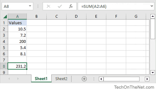
Based on the Excel spreadsheet above, the following SUM examples would return:

=SUM(A2:A6)
Result: 231.2

=SUM(A2, A3)
Result: 17.7

=SUM(A3, A5, 45)
Result: 57.6

=SUM(A2:A3, A5:A6)
Result: 31.2

=SUM(A2:A3, A5:A6, 500)
Result: 531.2

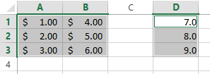
The SUM function is also a great function if you want to add values across a row. For example:

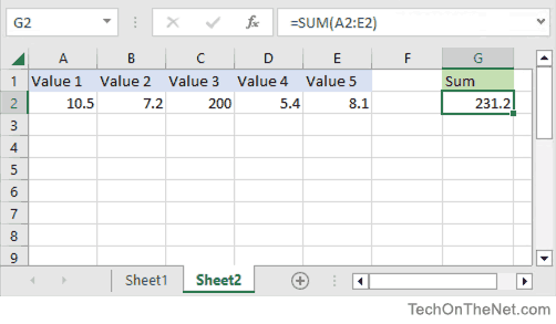
Based on the Excel spreadsheet above, the following SUM function would return:

=SUM(A2:E2)
Result: 231.2

Frequently Asked Questions

Question: I have a question about how to write the following formula in Excel.

I have a few cells, but I only need the sum of all the negative cells. So if I have 8 values, A1 to A8 and only A1, A4 and A6 are negative then I want B1 to be sum(A1,A4,A6).

Answer: You can use the SUMIF function to sum only the negative values as you described above. For example:

=SUMIF(A1:A8,"<0")

This formula would sum only the values in cells A1:A8 where the value is negative (ie: <0).

Источник

The SUM function concern into the category «Mathematical». Press the combination of hot keys SHIFT + F3 to call of the function wizard, and you will quickly search out it there.

The using of this function significantly expands to the possibilities of the process of summing the values of the cells in Excel. We look at the possibilities and settings for the summing several ranges practically.

How in the Excel table to calculate the amount of the column?

Sum up the value of the cells A1, A2 and A3 using the summation function and at the same time we will learn what the sum function is used for.

After entering the numbers, go to the cell A4. On the «Home» tab, select the «Sum» tool in the «Edit» section (or press the ALT + = hot keys combination).

The range of the cells is recognized automatically. The reference addresses are already entered in the parameters (A1:A3). The user only remains to press Enter.

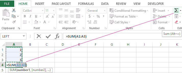
Consequently, the calculation result is displayed in the cell A4. The function itself and its parameters can be seen in the formula bar.

The notation. Instead of using the «Sum» tool on the main panel, you can directly enter the function with parameters manually in the cell A4. The result will be the same.

The Automatic Range Recognition Correction

When you enter of the function using the button on the toolbar or using the function wizard (SHIFT + F3), the SUM () function refers to the group of formulas «Mathematical». Automatically recognized ranges are not always suitable for the user: its can be quickly and easily repaired if necessary.

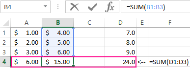
Suppose we need to sum several ranges of cells, as shown in the picture:

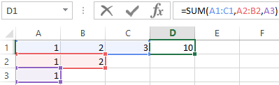
Go to the cell D1 and select the «Sum» tool.
While holding the CTRL key, select the range A2:B2 and the cell A3.
After selecting of the ranges, press Enter and in the cell D4 immediately displays the result of summing the values of cells in all ranges.

Pay attention to the syntax in the function parameters when selecting multiple ranges, that are divided among themselves (;).

In the SUM formula parameters may contain:

the links to individual cells;
the references to ranges of the cells both contiguous and non-adjacent;
the integer and fractional numbers.

In the function parameters, all arguments must be separated by a semicolon.

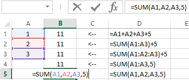
For the illustrative example, let’s consider different variants of summation of values of cells, that give the same result. To do this, fill the cells A1, A2 and A3 with numbers 1, 2 and 3 respectively. And fill the range of the cells B1:B5 with the following formulas and functions:

For any variant, we get the same result of calculation — the number 11. Continue successively with the cursor from B1 and to B5. In each cell, press F2 to see the color highlighting of the links for a more intuitive analysis of the syntax for writing parameters.

The contemporaneous summation of the columns

In Excel, you can simultaneously sum several adjacent and non-adjacent columns.

Fill in the columns, as shown in the picture:

Select the range A1:B3 and holding down the CTRL key also select the column D1:D3.
On the «HOME» panel, click the «Sum» tool (or press ALT + =).

Under each column, the SUM () was automatically added. Now in the cells A4;B4 and D4 the result of the summation of each column is displayed. This is the fastest and most convenient method.

The notation. This function automatically substitutes the format of the cells it sums.

Источник