
Excel for Microsoft 365 Excel 2021 Excel 2019 Excel 2016 Excel 2013 Excel 2010 Excel 2007 More…Less
Let’s say you want to ensure that a column contains text, not numbers. Or, perhapsyou want to find all orders that correspond to a specific salesperson. If you have no concern for upper- or lowercase text, there are several ways to check if a cell contains text.
You can also use a filter to find text. For more information, see Filter data.
Find cells that contain text
Follow these steps to locate cells containing specific text:
-
Select the range of cells that you want to search.
To search the entire worksheet, click any cell.
-
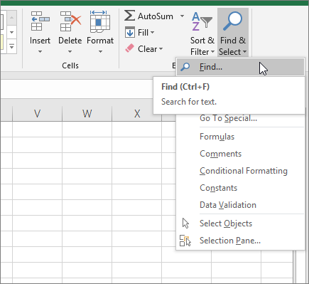
On the Home tab, in the Editing group, click Find & Select, and then click Find.

-
In the Find what box, enter the text—or numbers—that you need to find. Or, choose a recent search from the Find what drop-down box.
Note: You can use wildcard characters in your search criteria.
-
To specify a format for your search, click Format and make your selections in the Find Format popup window.
-
Click Options to further define your search. For example, you can search for all of the cells that contain the same kind of data, such as formulas.
In the Within box, you can select Sheet or Workbook to search a worksheet or an entire workbook.
-
Click Find All or Find Next.
Find All lists every occurrence of the item that you need to find, and allows you to make a cell active by selecting a specific occurrence. You can sort the results of a Find All search by clicking a header.
Note: To cancel a search in progress, press ESC.
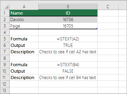
Check if a cell has any text in it
To do this task, use the ISTEXT function.
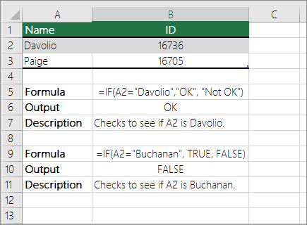
Check if a cell matches specific text
Use the IF function to return results for the condition that you specify.
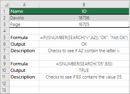
Check if part of a cell matches specific text
To do this task, use the IF, SEARCH, and ISNUMBER functions.
Note: The SEARCH function is case-insensitive.
Need more help?
Want more options?
Explore subscription benefits, browse training courses, learn how to secure your device, and more.
Communities help you ask and answer questions, give feedback, and hear from experts with rich knowledge.
Содержание
- Check if a cell contains text (case-insensitive)
- Find cells that contain text
- Check if a cell has any text in it
- Check if a cell matches specific text
- Check if part of a cell matches specific text
- Contains Specific Text
- How to spell check in Excel
- How to do spell check in Excel
- Spell check individual cells and ranges
- How to check spelling in multiple sheets
- How to spell check the entire workbook
- How to spell check text in formulas
- Spell check in Excel using a macro
- Macro to do spell check in the active sheet
- Macro to spell check all sheets of the active workbook
- Highlight misspelled words in Excel
- How to use spell checking macros
- Change the Excel spell check settings
- Excel spell check not working
- Spelling button is greyed out
- You are in edit mode
- Text in formulas is not checked
- Find typos and misprints with Fuzzy Duplicate Finder
Check if a cell contains text (case-insensitive)
Let’s say you want to ensure that a column contains text, not numbers. Or, perhapsyou want to find all orders that correspond to a specific salesperson. If you have no concern for upper- or lowercase text, there are several ways to check if a cell contains text.
You can also use a filter to find text. For more information, see Filter data.
Find cells that contain text
Follow these steps to locate cells containing specific text:
Select the range of cells that you want to search.
To search the entire worksheet, click any cell.
On the Home tab, in the Editing group, click Find & Select, and then click Find.
In the Find what box, enter the text—or numbers—that you need to find. Or, choose a recent search from the Find what drop-down box.
Note: You can use wildcard characters in your search criteria.
To specify a format for your search, click Format and make your selections in the Find Format popup window.
Click Options to further define your search. For example, you can search for all of the cells that contain the same kind of data, such as formulas.
In the Within box, you can select Sheet or Workbook to search a worksheet or an entire workbook.
Click Find All or Find Next.
Find All lists every occurrence of the item that you need to find, and allows you to make a cell active by selecting a specific occurrence. You can sort the results of a Find All search by clicking a header.
Note: To cancel a search in progress, press ESC.
Check if a cell has any text in it
To do this task, use the ISTEXT function.
Check if a cell matches specific text
Use the IF function to return results for the condition that you specify.
Check if part of a cell matches specific text
To do this task, use the IF, SEARCH, and ISNUMBER functions.
Note: The SEARCH function is case-insensitive.
Источник
Contains Specific Text
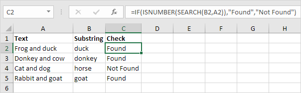
To check if a cell contains specific text, use ISNUMBER and SEARCH in Excel. There’s no CONTAINS function in Excel.
1. To find the position of a substring in a text string, use the SEARCH function.
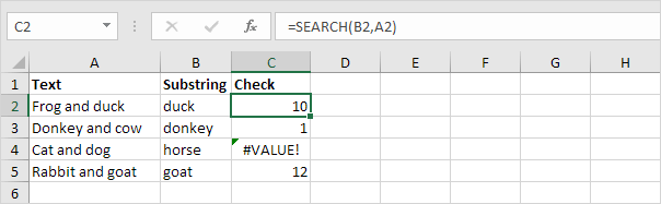
Explanation: «duck» found at position 10, «donkey» found at position 1, cell A4 does not contain the word «horse» and «goat» found at position 12.
2. Add the ISNUMBER function. The ISNUMBER function returns TRUE if a cell contains a number, and FALSE if not.
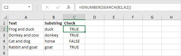
Explanation: cell A2 contains the word «duck», cell A3 contains the word «donkey», cell A4 does not contain the word «horse» and cell A5 contains the word «goat».
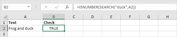
3. You can also check if a cell contains specific text, without displaying the substring. Make sure to enclose the substring in double quotation marks.
4. To perform a case-sensitive search, replace the SEARCH function with the FIND function.
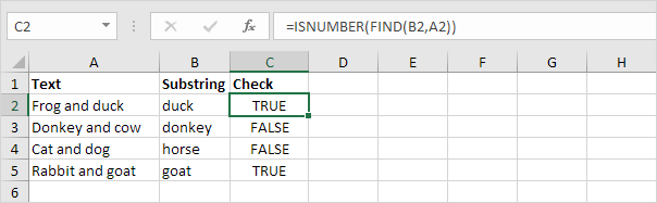
Explanation: the formula in cell C3 returns FALSE now. Cell A3 does not contain the word «donkey» but contains the word «Donkey».
5. Add the IF function. The formula below (case-insensitive) returns «Found» if a cell contains specific text, and «Not Found» if not.
6. You can also use IF and COUNTIF in Excel to check if a cell contains specific text. However, the COUNTIF function is always case-insensitive.

Explanation: the formula in cell C2 reduces to =IF(COUNTIF(A2,»*duck*»),»Found»,»Not Found»). An asterisk (*) matches a series of zero or more characters. Visit our page about the COUNTIF function to learn all you need to know about this powerful function.
Источник
How to spell check in Excel
 by Svetlana Cheusheva, updated on March 16, 2023
The tutorial shows how to perform spell check in Excel manually, with VBA code, and by using a special tool. You will learn how to check spelling in individual cells and ranges, active worksheet and the entire workbook.
Although Microsoft Excel is not a word processing program, it does have a few features to work with text, including the spell-checking facility. However, spell check in Excel is not exactly the same as in Word. It does not offer advanced capabilities like grammar checking, nor does it underline the misspelled words as you type. But still Excel provides the basic spell checking functionality and this tutorial will teach you how to get most of it.
How to do spell check in Excel
No matter which version you are using, Excel 2016, Excel 2013, Excel 2010 or lower, there are 2 ways to spell check in Excel: a ribbon button and a keyboard shortcut.
Simply, select the first cell or the cell from which you’d like to start checking, and do one of the following:
- Press the F7 key on your keyboard.
- Click the Spelling button on the Review tab, in the Proofing group.
This will perform a spelling check on the active worksheet: 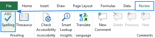
When a mistake is found, the Spelling dialog window shows up: 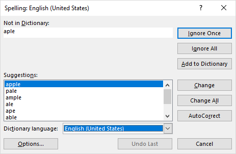
To correct a mistake, choose an appropriate opting under Suggestions, and click the Change button. The misspelt word will be replaced with the selected one and the next mistake will be brought to your attention.
If the «mistake» is not really a mistake, pick one of the following options:
- To ignore the current mistake, click Ignore Once.
- To ignore all the mistakes same as the current one, click Ignore All.
- To add the current word to dictionary, click Add to Dictionary. This will ensure that the same word won’t be treated as a mistake when you do a spell check next time.
- To replace all the mistakes same as the current one with the selected suggestion, click Change All.
- To let Excel correct the mistake as it sees fit, click AutoCorrect.
- To set another proofing language, select it from the Dictionary language drop box.
- To view or change the spell check settings, click the Options… button.
- To stop the correction process and close the dialog, click the Cancel button.
When the spell check is complete, Excel will show you the corresponding message: 
Spell check individual cells and ranges
Depending on your selection, Excel Spell check processes different areas of the worksheet:
By selecting a single cell, you tell Excel to perform spell check on the active sheet, including text in the page header, footer, comments, and graphics. The selected cell is the starting point:
- If you select the first cell (A1), the entire sheet is checked.
- If you select some other cell, Excel will start spell checking from that cell onward till the end of the worksheet. When the last cell is checked, you will be prompted to continue checking at the beginning of the sheet.
To spell check one particular cell, double-click that cell to enter the edit mode, and then initiate spell check.
To check spelling in a range of cells, select that range and then run the spell-checker.
To check only part of the cell contents, click the cell and select the text to check in the formula bar, or double click the cell and select the text in the cell.
How to check spelling in multiple sheets
To check several worksheets for spelling mistakes at a time, do the following:
- Select the sheet tabs you wish to check. For this, press and hold the Ctrl key while clicking the tabs.
- Press the spell check shortcut ( F7 ) or click the Spelling button on the Review tab.
Excel will check spelling mistakes in all the selected worksheets: 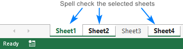
When the spell check is completed, right click the selected tabs and click Ungroup sheets.
How to spell check the entire workbook
To check spelling in all the sheets of the current workbook, right click on any sheet tab and pick Select all Sheets from the context menu. With all the sheets selected, press F7 or click the Spelling button on the ribbon. Yep, it’s that easy! 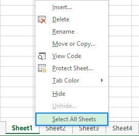
How to spell check text in formulas
Normally, Excel does not check formula-driven text because a cell actually contains a formula, not a text value: 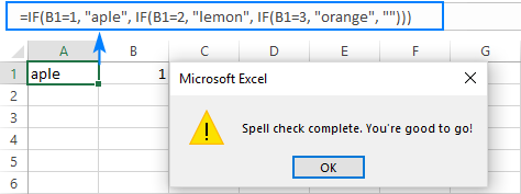
However, if you get in the edit mode and then run spell check, it will work: 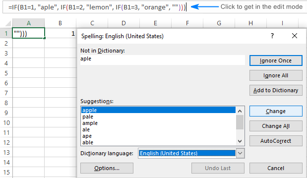
Of course, you will need to check each cell individually, which is not very good, but still this approach may help you eliminate spelling errors in big formulas, for example, in multi-level nested IF statements.
Spell check in Excel using a macro
If you like automating things, you can easily automate the process of finding wrongly spelled words in your worksheets.
Macro to do spell check in the active sheet
What can be simpler than a button click? Maybe, this line of code 🙂
Macro to spell check all sheets of the active workbook
You already know that to search for spelling mistakes in multiple sheets, you select the corresponding sheet tabs. But how do you check hidden sheets?
Depending on your target, use one of the following macros.
To check all visible sheets:
To check all sheets in the active workbook, visible and hidden:
Highlight misspelled words in Excel
This macro allows you to find the misspelled words simply by viewing the sheet. It highlights the cells containing one or more spelling mistakes in red. To use another background color, change the RGB code in this line: cell.Interior.Color = RGB(255, 0, 0).
How to use spell checking macros
Download our sample workbook with Spell Check macros, and perform these steps:
- Open the downloaded workbook and enable the macros if prompted.
- Open your own workbook and switch to the worksheet you want to check.
- Press Alt + F8 , select the macro, and click Run.
The sample workbook contains the following macros:
- SpellCheckActiveSheet — performs a spell check in the active worksheet.
- SpellCheckAllVisibleSheets — checks all visible sheets in the active workbook.
- SpellCheckAllSheets — checks visible and invisible sheets in the active workbook.
- HighlightMispelledCells — changes the background color of cells that contain wrongly spelled words.
You can also add the macros to you own sheet by following these instructions: How to insert and run VBA code in Excel.
For example, to highlight all the cells with spelling errors in the current spreadsheet, run this macro: 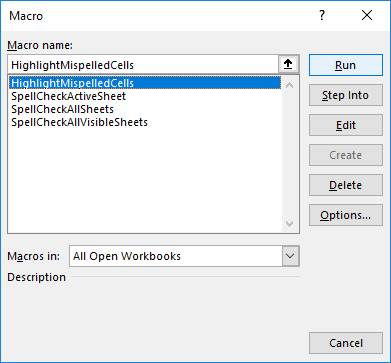
And get the following result: 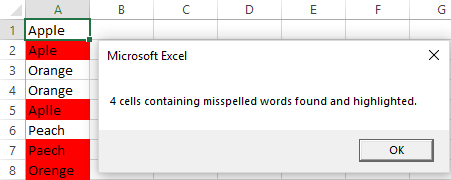
Change the Excel spell check settings
If you’d like to tweak the behavior of spell check in Excel, click File > Options > Proofing, and then check or uncheck the following options:
- Ignore words in uppercase
- Ignore words that contain numbers
- Ignore internet files and addresses
- Flag repeated words
All the options are self-explanatory, maybe except the language-specific ones (I can explain about enforcing strict ё in the Russian language if someone cares 🙂
The screenshot below shows the default settings: 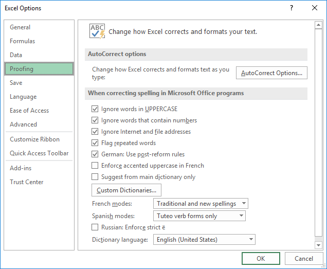
Excel spell check not working
If spell check does not work properly in your worksheet, try these simple troubleshooting tips:
Spelling button is greyed out
Most likely your worksheet is protected. Excel spell check does not work in protected sheets, so you will have to unprotect your worksheet first.
You are in edit mode
When in edit mode, only the cell you are currently editing is checked for spelling errors. To check the whole worksheet, exit the edit mode, and then run spell check.
Text in formulas is not checked
Cells containing formulas are not checked. To spell check text in a formula, get in the edit mode.
Find typos and misprints with Fuzzy Duplicate Finder
In addition to the built-in Excel spell check functionality, the users of our Ultimate Suite can quickly find and fix typos by using a special tool that resides on the Ablebits Tools tab under Find and Replace: 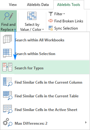
Clicking the Search for Typos button opens the Fuzzy Duplicate Finder pane on the left side of your Excel window. You are to select the range to check for typos and configure the settings for your search:
- Max number of different characters — limit the number of differences to look for.
- Min number of characters in a word/cell — exclude very short values from the search.
- The cells contain separate words delimited by — select this box if your cells may contain more than one word.
With the settings properly configured, click the Search for typos button. 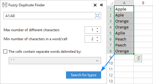
The add-in starts searching for values that differ in 1 or more characters, as specified by you. Once the search is finished, you are presented with a list of the found fuzzy matches grouped in nodes like shown in the screenshot below.
Now, you are to set the correct value for each node. For this, expand the group, and click the check symbol in the Action column next to the right value: 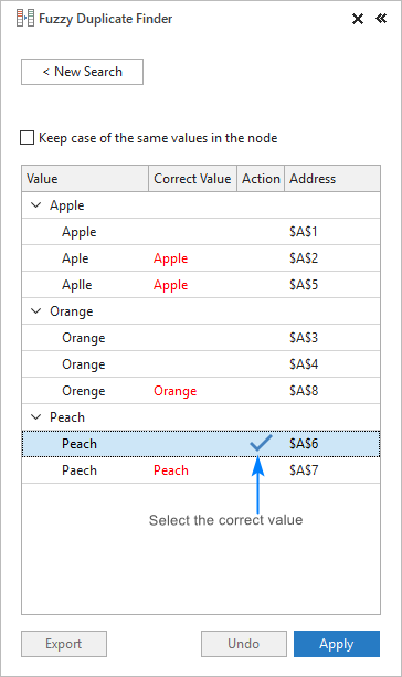
If the node doesn’t contain the right word, click in the Correct Value box next to the root item, type the word, and press Enter . 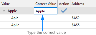
Upon assigning the correct values to all the nodes, click the Apply button, and all the typos in your worksheet will be fixed in one go: 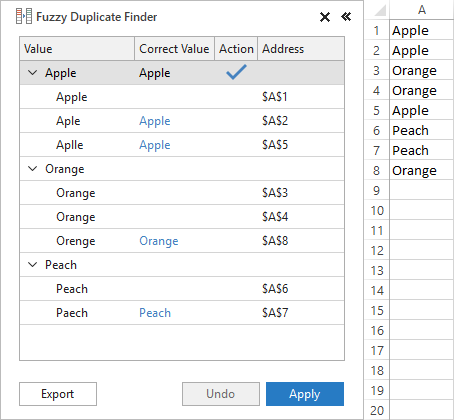
That’s how you perform spell check in Excel with Fuzzy Duplicate Finder. If you are curious to try this and 70+ more professional tools for Excel, you are welcome to download a trial version of our Ultimate Suite.
Источник
![]()
Excel If Cell Contains Text

Excel If Cell Contains Text Then Formula helps you to return the output when a cell have any text or a specific text. You can check if a cell contains a some string or text and produce something in other cell. For Example you can check if a cell A1 contains text ‘example text’ and print Yes or No in Cell B1. Following are the example Formulas to check if Cell contains text then return some thing in a Cell.
If Cell Contains Text
Here are the Excel formulas to check if Cell contains specific text then return something. This will return if there is any string or any text in given Cell. We can use this simple approach to check if a cell contains text, specific text, string, any text using Excel If formula. We can use equals to operator(=) to compare the strings .
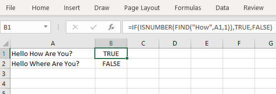
If Cell Contains Text Then TRUE
Following is the Excel formula to return True if a Cell contains Specif Text. You can check a cell if there is given string in the Cell and return True or False.
The formula will return true if it found the match, returns False of no match found.
If Cell Contains Partial Text
We can return Text If Cell Contains Partial Text. We use formula or VBA to Check Partial Text in a Cell.
Find for Case Sensitive Match:
We can check if a Cell Contains Partial Text then return something using Excel Formula. Following is a simple example to find the partial text in a given Cell. We can use if your want to make the criteria case sensitive.
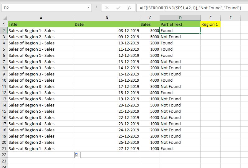
- Here, Find Function returns the finding position of the given string
- Use Find function is Case Sensitive
- IsError Function check if Find Function returns Error, that means, string not found
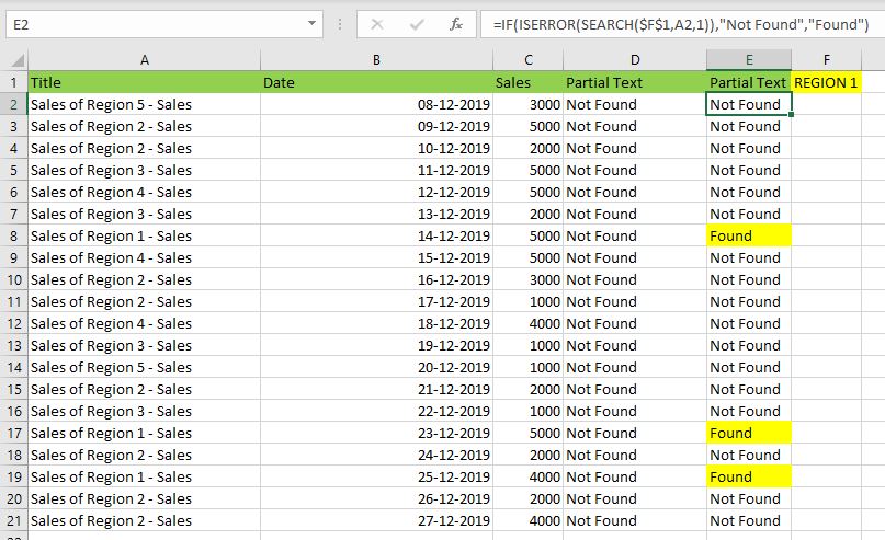
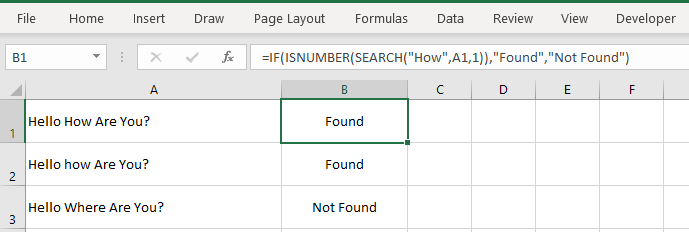
Search for Not Case Sensitive Match:
We can use Search function to check if Cell Contains Partial Text. Search function useful if you want to make the checking criteria Not Case Sensitive.
If Range of Cells Contains Text
We can check for the strings in a range of cells. Here is the formula to find If Range of Cells Contains Text. We can use Count If Formula to check the excel if range of cells contains specific text and return Text.
- CountIf function counts the number of cells with given criteria
- We can use If function to return the required Text
- Formula displays the Text ‘Range Contains Text” if match found
- Returns “Text Not Found in the Given Range” if match not found in the specified range
If Cells Contains Text From List
Below formulas returns text If Cells Contains Text from given List. You can use based on your requirement.
VlookUp to Check If Cell Contains Text from a List:
We can use VlookUp function to match the text in the Given list of Cells. And return the corresponding values.
- Check if a List Contains Text:
=IF(ISERR(VLOOKUP(F1,A1:B21,2,FALSE)),”False:Not Contains”,”True: Text Found”) - Check if a List Contains Text and Return Corresponding Value:
=VLOOKUP(F1,A1:B21,2,FALSE) - Check if a List Contains Partial Text and Return its Value:
=VLOOKUP(“*”&F1&”*”,A1:B21,2,FALSE)
If Cell Contains Text Then Return a Value
We can return some value if cell contains some string. Here is the the the Excel formula to return a value if a Cell contains Text. You can check a cell if there is given string in the Cell and return some string or value in another column.
The formula will return true if it found the match, returns False of no match found. can
Excel if cell contains word then assign value
You can replace any word in the following formula to check if cell contains word then assign value.
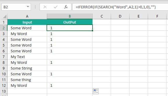
Search function will check for a given word in the required cell and return it’s position. We can use If function to check if the value is greater than 0 and assign a given value (example: 1) in the cell. search function returns #Value if there is no match found in the cell, we can handle this using IFERROR function.
Count If Cell Contains Text
We can check If Cell Contains Text Then COUNT. Here is the Excel formula to Count if a Cell contains Text. You can count the number of cells containing specific text.
The formula will Sum the values in Column B if the cells of Column A contains the given text.
Count If Cell Contains Partial Text
We can count the cells based on partial match criteria. The following Excel formula Counts if a Cell contains Partial Text.
- We can use the CountIf Function to Count the Cells if they contains given String
- Wild-card operators helps to make the CountIf to check for the Partial String
- Put Your Text between two asterisk symbols (*YourText*) to make the criteria to find any where in the given Cell
- Add Asterisk symbol at end of your text (YourText*) to make the criteria to find your text beginning of given Cell
- Place Asterisk symbol at beginning of your text (*YourText) to make the criteria to find your text end of given Cell
If Cell contains text from list then return value
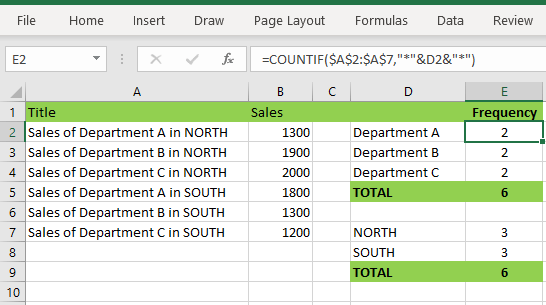
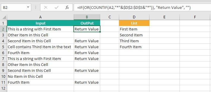
Here is the Excel Formula to check if cell contains text from list then return value. We can use COUNTIF and OR function to check the array of values in a Cell and return the given Value. Here is the formula to check the list in range D2:D5 and check in Cell A2 and return value in B2.
If Cell Contains Text Then SUM
Following is the Excel formula to Sum if a Cell contains Text. You can total the cell values if there is given string in the Cell. Here is the example to sum the column B values based on the values in another Column.
The formula will Sum the values in Column B if the cells of Column A contains the given text.

Sum If Cell Contains Partial Text
Use SumIfs function to Sum the cells based on partial match criteria. The following Excel formula Sums the Values if a Cell contains Partial Text.
- SUMIFS Function will Sum the Given Sum Range
- We can specify the Criteria Range, and wild-card expression to check for the Partial text
- Put Your Text between two asterisk symbols (*YourText*) to Sum the Cells if the criteria to find any where in the given Cell
- Add Asterisk symbol at end of your text (YourText*) to Sum the Cells if the criteria to find your text beginning of given Cell
- Place Asterisk symbol at beginning of your text (*YourText) to Sum the Cells if criteria to find your text end of given Cell
VBA to check if Cell Contains Text
Here is the VBA function to find If Cells Contains Text using Excel VBA Macros.
If Cell Contains Partial Text VBA
We can use VBA to check if Cell Contains Text and Return Value. Here is the simple VBA code match the partial text. Excel VBA if Cell contains partial text macros helps you to use in your procedures and functions.
MsgBox CheckIfCellContainsPartialText(Cells(2, 1), “Region 1”)
End Sub
Function CheckIfCellContainsPartialText(ByVal cell As Range, ByVal strText As String) As Boolean
If InStr(1, cell.Value, strText) > 0 Then CheckIfCellContainsPartialText = True
End Function
- CheckIfCellContainsPartialText VBA Function returns true if Cell Contains Partial Text
- inStr Function will return the Match Position in the given string
If Cell Contains Text Then VBA MsgBox
Here is the simple VBA code to display message box if cell contains text. We can use inStr Function to search for the given string. And show the required message to the user.
If InStr(1, Cells(2, 1), “Region 3”) > 0 Then blnMatch = True
If blnMatch = True Then MsgBox “Cell Contains Text”
End Sub
- inStr Function will return the Match Position in the given string
- blnMatch is the Boolean variable becomes True when match string
- You can display the message to the user if a Range Contains Text
Which function returns true if cell a1 contains text?
You can use the Excel If function and Find function to return TRUE if Cell A1 Contains Text. Here is the formula to return True.
Which function returns true if cell a1 contains text value?
You can use the Excel If function with Find function to return TRUE if a Cell A1 Contains Text Value. Below is the formula to return True based on the text value.
Share This Story, Choose Your Platform!
7 Comments
-
Meghana
December 27, 2019 at 1:42 pm — ReplyHi Sir,Thank you for the great explanation, covers everything and helps use create formulas if cell contains text values.
Many thanks! Meghana!!
-
Max
December 27, 2019 at 4:44 pm — ReplyPerfect! Very Simple and Clear explanation. Thanks!!
-
Mike Song
August 29, 2022 at 2:45 pm — ReplyI tried this exact formula and it did not work.
-
Theresa A Harding
October 18, 2022 at 9:51 pm — Reply -
Marko
November 3, 2022 at 9:21 pm — ReplyHi
Is possible to sum all WA11?
(A1) WA11 4
(A2) AdBlue 1, WA11 223
(A3) AdBlue 3, WA11 32, shift 4
… and everything is in one column.
Thanks you very much for your help.
Sincerely Marko
-
Mike
December 9, 2022 at 9:59 pm — ReplyThank you for the help. The formula =OR(COUNTIF(M40,”*”&Vendors&”*”)) will give “TRUE” when some part of M40 contains a vendor from “Vendors” list. But how do I get Excel to tell which vendor it found in the M40 cell?
-
PNRao
December 18, 2022 at 6:05 am — ReplyPlease describe your question more elaborately.
Thanks!
-
© Copyright 2012 – 2020 | Excelx.com | All Rights Reserved
Page load link
Smart searching makes the whole search process a breeze and that’s smart stuff for you, making everything easy breezy. As your search gets specific, the process gets more complicated and if you don’t employ the right techniques, you’ll find yourself having a bad fishing day in a ginormous Excel sea. See if you can get it right the first time with what we have planned for you here today.
Your learning today comprises checking cells for partial text using the SEARCH, COUNTIF, and MATCH functions along with other functions to control the outcome. Find out how to use wildcard characters to aid the search. We’ll use a case example to give the explanations a visual touch. 1")
Case Example
Enlisted ahead in the example shot, we have our stock of fragrances. The fragrances are alphabetically sorted by name and the slight problem here is that the brand is also mentioned in the same cell. Now if we are to find fragrances according to a brand, we can’t do it as easily.
 2")
A start can be to split the brands from the names into a separate column but even then, we have a problem. If we alphabetically sort the brand names and search for a fragrance by Armani, our search will turn up pointless because the fragrance is listed by the name of Giorgio Armani and would be lying in the range of G while we’d be searching the brands with A as the initials.
So we need something a little more foolproof for our searches and we’ve expounded these ideas ahead in this tutorial.
Let’s get checking!
Using SEARCH Function
Partial text in a cell can be checked with the SEARCH function. The SEARCH function searches a cell for a given value and returns the position of the character at which the value is found. That’s how the SEARCH function will work on its own but there are ways to use the SEARCH function to expand its usability.
We can better look into this with an example so let’s merge our case example with the SEARCH function and apply the formula below:
=IF(ISNUMBER(SEARCH("Chanel",B3)),"Yes","-")
First we’ll talk about the SEARCH function. We want to find fragrances by Chanel in our stock and we have fed this brand name in the formula. The point of search is column B hence, the first cell to search is B3. Technically this should be enough, right? Let’s apply just the SEARCH function and see if it works:
 3")
Now that works… partially. The SEARCH function returns the position of the character where Chanel is found i.e. the 9th character. Since SEARCH couldn’t return the character’s position in the first instance (because B3 doesn’t contain the value «Armani»), it results in the #VALUE! error. While the SEARCH function on its own does something to give us the idea that the searched value is there, we need something more suitable for our spreadsheets.
Incoming: the ISNUMBER function. ISNUMBER returns TRUE when the provided value is a number and FALSE when it isn’t. This way, the ISNUMBER function will result in TRUE when SEARCH results in a numeric value and FALSE otherwise.
But we’re going for further prominence in the results and that’s why we’ve wrapped everything in the IF function. The IF function will yield a «Yes» upon finding «Chanel» as part of the cell value. Otherwise it will yield a dash «-«
 4")
With more clarity, we can easily see that we have 3 Chanel fragrances in stock.
Notes:
The SEARCH function doesn’t require a wildcard asterisk but a wildcard question mark can be used to replace a single character. Find out what a wildcard character is in the COUNTIF function section.
The SEARCH function is not case-sensitive. Switch it out with the FIND function for a case-sensitive option.
Checking Two Values
Checking our stock for Chanel was one value. Let’s also search for Gucci fragrances because why not? For searching two values, we will need the OR function. The OR function returns TRUE if any of the specified conditions are met and FALSE if none are met. Now see the formula with the SEARCH function for checking if a cell contains either of the two values:
=IF(OR(ISNUMBER(SEARCH("Chanel",B3)),ISNUMBER(SEARCH("Gucci",B3))),"Yes","-")
We’re finding two values so the formula has 2 SEARCH formulas; one with Chanel as the search value and one with Gucci. Both the SEARCH formulas are controlled by the ISNUMBER function. The OR function is fed with two conditions; find Chanel or find Gucci. If either is found, the IF function makes sure that «Yes» is returned. Else, a dash is returned.
 5")
Note: Suppose instead of finding two values in separate cells, you want to find two values in the same cell. E.g. we’re unable to recall the full name of a fragrance by Chanel but remember that the name included «de». In that case, the OR function will be replaced by the AND function and the search values will be «Chanel» and «de».
=IF(AND(ISNUMBER(SEARCH("Chanel",B3)),ISNUMBER(SEARCH("de",B3))),"Yes","-")
Using COUNTIF Function
An alternative to the SEARCH function for checking partial text in a cell is the COUNTIF function. The COUNTIF function is used to count the cells that meet a given condition. COUNTIF makes a lighter formula for finding partially matching text since the ISNUMBER function can be dropped.
The added touch is, however, having to use a wildcard character to match zero or more characters. In the coming sections, we’ll show you how to use the wildcard characters (the asterisk and question mark) within the COUNTIF function to check if a cell contains certain text.
Wildcard Characters
With Asterisk
The COUNTIF function needs to be triggered for searching part of the text in a cell with the asterisk in the formula. The asterisk acts as a replacement for zero or more characters and without it, the formula will search a cell containing just search text instead of searching a cell that includes the search text. The asterisk will be placed depending on the position of the text you want to find within the cell. Here’s a little helper:
| Criterion | Parameter in the formula |
|---|---|
| Find text at the beginning of a cell | «text*» |
| Find text in the middle or anywhere in the cell | «*text*» |
| Find text at the end of a cell | «*text» |
Judging from the above, the asterisk can also be placed at the end of Chanel if we’re unsure of any text after it in the cell. A safer bet will be to enclose the search text in asterisks because the presence of one can always account for zero characters but the absence will mean that there is no text.
Let’s proceed to the formula now so you can see how this works:
=IF(COUNTIF(B3,"*Chanel"),"Yes","-")
The COUNTIF function is to return 1 for a cell containing «*Chanel». The asterisk is placed before the text of interest because we know that the brand name will be the last part of the text in the cell. If the cell does not contain Chanel as the last of the text, COUNTIF will return 0.
To customize 1 and 0, we have added the IF function in the formula to replace these numbers with «Yes» and «-» respectively. These are the results:
 6")
Search a Range
In the case above, we were seeing which fragrances by Chanel were in stock. If we were only out to check whether the stock contained any Chanel fragrances at all, without specificity, we can apply the COUNTIF function to the whole range in the dataset and get a single cell result in return. In Excel words, the COUNTIF function works on a range as well as a single cell. Use this formula to check a range for partial matching:
=IF(COUNTIF(B3:B12,"*Chanel"),"Yes","-")
The only thing we have changed in this formula is the cell reference from B3 to the range B3:B12. The formula searches this range for cells that contain Chanel as the ending text. Since there are 3 cells in this range that meet this condition, the formula gives us a «Yes» in a single cell.
 7")
With Question Mark
Another wildcard character with an interesting characteristic is the question mark. While the asterisk can signify multiple characters, a single question mark signifies a single character and more than one can be used.
Let’s draw from our case example. We are certain there is a Lancome fragrance in our stock but can’t quite remember what spelling the entry has been made with. Was it Lancôme or Lancome? Don’t sweat it. It’s just the O causing dubiety and we can replace it with a question mark wildcard. Use a formula like this to check for partial matching using a wildcard question mark:
=IF(COUNTIF(B3,"*Lanc?me"),"Yes","-")
Only changing our search text in this formula, the rest is the same COUNTIF we were using earlier. Now we are searching for a Lancome fragrance with a leading asterisk because the remaining text is before the brand name in the cell. The dubious «o» in Lancome has been replaced with a question mark.
Applying this formula to all the fragrances in our dataset, we have one «Yes» returned for B11, solving our mystery spelling as Lancôme.
 8")
Notes:
The COUNTIF function works for ranges too so it can also be applied as a range formula, depending on what your requirement is.
Using MATCH Function
The last option for checking a cell that may contain your search text in part is the MATCH function. The MATCH function checks an array for a value and returns the position of the cell in that array. We can work with that. If the position of the cell in the array is what we insist on, then we can do with using just the MATCH function. But we’re finding a specific text in a range so we’ll throw more spanners into the works. Keep reading!
Wildcard Characters
With Asterisk
With the MATCH function, we also need to use the asterisk as a wildcard. We require other functions like in this formula ahead:
=IF(ISNA(MATCH("*Chanel*",B3:B12,0)),"Not Found!","Found")
The MATCH function has been equipped with Chanel as the first parameter enclosed in two asterisks to replace possible text. The lookup array is B3:B12 and 0 has been entered to find an exact match. When the search text cannot be found, MATCH will result in a #N/A error and for finding every match, 1 will be returned.
To channel #N/A and 1 into TRUE and FALSE, the ISNA function has been added in the formula. the ISNA function returns TRUE when a value is #N/A. Now the TRUE and FALSE are in guise with «Not Found!» and «Found» by the IF function respectively.
The MATCH function picked up on 3 cells that contain the text Chanel. ISNA checks for an #N/A error. Since MATCH’s result is 3, there is no #N/A error – leading to FALSE. The value for FALSE as per the IF function is «Found». The indication is that the search text Chanel has been found in the range B3:B12.
 9")
The same formula can be used with the range excluded and relative cell reference included to find the exact cells that contain the matching text:
=IF(ISNA(MATCH("*Chanel*",B3,0)),"Not Found!","Found")
 10")
With Question Mark
Now let’s see how to use the question mark as a wildcard character with the MATCH function for finding partial text in a range.
=IF(ISNA(MATCH("*Lanc?me",B3:B12,0)),"Not Found!","Found")
With the same lineup of the MATCH, ISNA, and IF functions, we’ve entered the search text with a wildcard question mark to find Lanc?me in B3:B12. And good news, it has been found.
 11")
Open up the results by using a cell reference instead of the range to specifically find the cell that contains the Lanc?me fragrance:
=IF(ISNA(MATCH("*Lanc?me",B3:B12,0)),"Not Found!","Found")
 12")
One more thing this tutorial contains is the end of the tutorial so we’re heading out of finding partial matches in text in Excel. But if this is new for you, get cracking with some text search experiments and before you’re ready to head out, we’ll be back with more Excel stuff to crack. You can count on us for that!
This is an old question but a solution for those using Excel 2016 or newer is you can remove the need for nested if structures by using the new IFS( condition1, return1 [,condition2, return2] ...) conditional.
I have formatted it to make it visually clearer on how to use it for the case of this question:
=IFS(
ISERROR(SEARCH("String1",A1))=FALSE,"Something1",
ISERROR(SEARCH("String2",A1))=FALSE,"Something2",
ISERROR(SEARCH("String3",A1))=FALSE,"Something3"
)
Since SEARCH returns an error if a string is not found I wrapped it with an ISERROR(...)=FALSE to check for truth and then return the value wanted. It would be great if SEARCH returned 0 instead of an error for readability, but thats just how it works unfortunately.
Another note of importance is that IFS will return the match that it finds first and thus ordering is important. For example if my strings were Surf, Surfing, Surfs as String1,String2,String3 above and my cells string was Surfing it would match on the first term instead of the second because of the substring being Surf. Thus common denominators need to be last in the list. My IFS would need to be ordered Surfing, Surfs, Surf to work correctly (swapping Surfing and Surfs would also work in this simple example), but Surf would need to be last.