Checking dates in excel

Data analysis in Excel often involves working with dates.

A common thing many Excel users need to check when working with dates is whether a date is between two given dates.

A simple use case of this could be when you need to check whether the date of submission of a report was within the given dates or not. Based on this, you can highlight what reports were submitted after the deadline.

In this tutorial, I will show you how to check if the date is between two given dates or not.

Using Nested IF Formula

One of the easiest ways to check whether a date is in between two given dates is by using a simple if formula.

And since we need to check for two conditions, we would need to use two if formulas.

And when you use an IF formula within another IF formula, that is called the nested IF construct.

Below I have a data set where I have the project start date and project end date in column A and column B respectively. And then I have the project submission date in column C.

Now I want to check whether the project submission date was between the project start and project end date or not.

This can easily be done using the below nested IF formula:

=IF(C2>=A2,IF(C2<=B2,"In Range","Out of Range"),"Out of Range")

The above formula would return ‘In Range’ if the date lies in between the two given dates, and it would return ‘Out of Range’ in case the date is either before the project started or after the project end date.

Now let me quickly explain how this formula works.

I first used and if formula to check whether the date is after the project start date or not.

Based on these criteria, I need to specify what should the formula do in case this condition is true, and what should the formula do in case the condition is not true.

But since I have two conditions to check, immediately after I checked the first condition, I use the second IF function to check for the other condition (which is whether the date is before the project end date or not).

Since the IF function takes 3 arguments (the condition, value when the condition is True, and value in the condition is False), for the second IF function, I specify ‘In Range’ as the second argument, as it has satisfied both the conditions, and I specify out of range as the third argument, because it satisfies the first if condition, but it fails the second if condition.

And then finally, I specify ‘Out of Range’ as the second argument for the first IF function (which means that the condition in the first IF function failed, and hence it did not go to the second if function and instead returned the second argument of the first IF function).

Since I had only two conditions to check, I have used two if functions where the second function is nested within the first one. In case you have more than two conditions to check you can further nest these if functions (although it tends to get a bit complicated after a few)

Also read: Avoid Nested IF Function in Excel…VLOOKUP to Rescue

Using IF + AND Formula

While many Excel users are quite comfortable using the IF formula, when you have multiple conditions to check, I prefer using the combination of IF and AND formula instead.

Within the AND formula, you can check for multiple conditions, and can specify what result you should get in case all the conditions are true, and the result you should get in case any of these conditions are FALSE.

Let’s again take the same data set where I have the project started and project end date in column A and column B, and I have the project submission date in column C.

Below is the formula I can use to check whether the submission date lies between the project start date and project end date or not:

=IF(AND(C2>=A2,C2<=B2),"In Range","Out of Range")

The above formula checks for both the conditions and it would return ‘In Range’ in case the submission date is in between the start and the end date, and it would return ‘Out of Range’ in case the submission date is before the project started or after the project end date.

Note that I have still used an IF function in the above formula, however, I didn’t have the need to use two if functions.

Since I had to check for both the conditions, I did that using the AND function instead.

The AND function would return TRUE if both the conditions are true, and it would return FALSE if any or both the conditions are false.

And since I needed a more descriptive output instead of a simple TRUE or FALSE, I have used an IF function where it would give me ‘In Range’ in case the result is TRUE and ‘Out of Range’ in case the result is FALSE.

Check If the Date Occurs on Weekend

A common use case when working with dates in project management is to identify whether a date occurs on a weekend or not.

If you’re checking this manually, you would check whether a date is a Saturday or Sunday.

But when working with dates in Excel, you can use the WEEKDAY function that can easily do this for you.

Below I have a data set where I have some dates in column A, and I want to check whether these dates occur on a weekend or not.

For the purpose of this tutorial, I would consider Saturday and Sunday as the weekend days.

Below is the formula that will do this for you:

=WEEKDAY(A2,2)>5

If the date occurs on a Saturday or Sunday, it will give you a TRUE, else it will give a FALSE.

The above WEEKDAY formula checks the serial number of the date, and returns a number that corresponds to the weekday number for that date. So if it’s a Monday, it would return 1, if it’s a Tuesday it would return 2, and so on.

Since the condition that I’m checking is whether the weekday result is more than 5, it would return TRUE if the date is on a weekend, and it would return FALSE if it’s on a weekday.

If you want the result to be more meaningful, you can use the below if formula, which will return ‘Weekday’ in case the date occurs on a weekday and ‘Weekend’ in case the date occurs on a weekend.

=IF(WEEKDAY(A2,2)>5,"Weekend","Weekday")

Issues When Checking Whether a Date is in Between two dates

So far, I’ve shown you a couple of scenarios where you can check whether a date lies between two given dates.

In all the formulas, the underlying principle is to compare the value of the given date with the start and the end date. If the value of the given date, is in between the start and the end date, then it occurs in between these two dates, else it does not.

However, in some cases, you may see some unexpected results.

In this section, I cover some common pitfalls that you need to be aware of when comparing dates in Excel:

Dates Need to Be in the Right Format

Dates and time values are stored as numbers in the back-end in Excel. So when you compare two dates, you’re essentially comparing two numbers.

You may think that the date looks nothing like a number (for example 01 January 2023), but remember that dates are formatted to show up differently in the cell in Excel, while in the back-end these are still numbers.

For example, a cell may show 01 January 2023, but in the backend, the value of this cell would be 44927 (which indicates the total number of days that have elapsed after 01 Jan 1900).

Now, if your dates are in the right format, all is well.

But there is also a possibility that your date is in a format that Excel does not recognize as a date, which means that instead of a number in the back end, it ends up being considered a text string.

For example, Jan 01, 2023, is not a valid date format in Excel.

So if you have this in a cell in excel, it would be considered a text string, and using this to compare it with other dates can give you incorrect results.

Bottom line – When comparing dates in Excel, make sure that the dates are in the right format

Also read: How to Change Date Format In Excel?

Dates May have a Time Part that’s Hidden

Just like dates, time values are also stored as numbers in the backend in Excel.

While a whole number would indicate a full day, the decimal part would indicate the portion of the day or the time value for that day.

For example, if you have 01-01-2023 18:00:00 in a cell in Excel, in the backend it would be 44927.75, where 44927 means 01-01-2023 and 0.75 means 18:00:00

Now, here’s the problem that you can encounter when checking whether a date lies in between two given dates.

You may clearly see that the date is in between the two given dates, but Excel may give you a different result.

This can happen because most of the time when people work with dates and times, the time portion is hidden so that you only see the date but you do not see the time value.

Below I have a simple example where I have the same date in cells A1 and B1, but when I compare these two cells, it tells me these are not the same.

While you can clearly see that these dates are exactly the same, what you do not see is that there is a time value in cell A1 that is hidden so you do not see it. But when excel compares these two cells, it considers these as different (which it rightly should).

While this is not such a common scenario, if this happens, it can sometimes stump even advanced Excel users.

In this tutorial, I showed you a couple of simple formulas that you can use to check whether a date is between two given dates or not.

I’ve also mentioned some of the pitfalls you should be aware of when comparing dates and Excel.

I hope you found this Excel tutorial useful.

Other Excel Tutorials you may also like:

• Calculate the Number of Months Between Two Dates in Excel
• How to Calculate the Number of Days Between Two Dates in Excel
• How to Add or Subtract Days to a Date in Excel
• How to Stop Excel from Changing Numbers to Dates Automatically
• How to Add Months to Date in Excel
• How to Get the Number of Days in a Month in Excel?
• Get Day Name from Date in Excel

The IF function is one of the most useful Excel functions. It is used to test a condition and return one value if the condition is TRUE and another if it is FALSE.

One of the most common applications of the IF function involves the comparison of values.

These values can be numbers, text, or even dates. However, using the IF statement with date values is not as intuitive as it may seem.

In this tutorial, I will demonstrate some ways in which you can use the IF function with date values.

Syntax and Usage of the IF Function in Excel

The syntax for the IF function is as follows:

IF(logical_test, [value_if_true], [value_if_false])

Here,

• logical_test is the condition or criteria that you want the IF function to test. The result of this parameter is either TRUE or FALSE
• value_if_true is the value that you want the IF function to return if the logical_test evaluates to TRUE
• value_if_false is the value that you want the IF function to return if the logical_test evaluates to FALSE

For example, say you want to write a statement that will return the value “yes” if the value in cell reference A2 is equal to 10, and “no” if it’s anything but 10.

You can then use the following IF function for this scenario:

=IF(A2=10,"yes","no")

Comparing Dates in Excel (Using Operators)

Unlike numbers and strings, comparison operators, when used with dates, have a slightly different meaning.

Here are some of the comparison operators that you can use when comparing dates, along with what they mean:

Operator	What it Means When Using with Dates
<	Before the given date
=	Same as the date with which we are comparing
>	After the given date
<=	Same as or before the given date
>=	Same as or after the given date

It may look like IF formulas for dates are the same as IF functions for numeric or text values, since they use the same comparison operators.

However, it’s not as simple as that.

Unfortunately, unlike other Excel functions, the IF function cannot recognize dates.

It interprets them as regular text values.

So you cannot use a logical test such as “>05/07/2021” in your IF function, as it will simply see the value “05/07/2021” as text.

Here are a few ways in which you can incorporate date values into your IF function’s logical_test parameter.

Using the IF Function with DATEVALUE Function

If you want to use a date in your IF function’s logical test, you can wrap the date in the DATEVALUE function.

This function converts a date in text format to a serial number that Excel can recognize as a date.

If you put a date within quotes, it is essentially a text or string value.

When you pass this as a parameter to the DATEVALUE function, it takes a look at the text inside the double quotes, identifies it as a date and then converts it to an actual Excel date value.

Let us say you have a date in cell A2, and you want cell B2 to display the value “done” if the date comes before or on the same date as “05/07/2021” and display “not done” otherwise.

You can use the IF function along with DATEVALUE in cell B2 as follows:

=IF(A2<DATEVALUE("05/07/2021"),"done","not done")

Here’s a screenshot to illustrate the effect of the above formula:

Using the IF Function with the TODAY Function

If you want to compare a date with the current date, you can use the IF function with the TODAY function in the logical test.

Let’s say you have a date in cell A2 and you want cell B2 to display the value “done” if it is a date before today’s date.

If not, you want let’s say you want to display the value “not done”. You can use the IF function along with the TODAY function in cell B2 as follows:

=IF(A2<TODAY(),"done","not done")

Here’s a screenshot to illustrate the effect of the above formula (assuming the current date is 05/08/2021):

Using the IF Function with Future or Past Dates

An interesting thing about dates in Excel is that you can perform addition and subtraction operations with them too.

This is because dates are basically stored in Excel as serial numbers, starting from the date Jan 1, 1900.

Each day after that is represented by one whole number.

So, the serial number 2 corresponds to Jan 2, 1900, and so on.

This means that adding n number of days to a date is equivalent to adding the value n to the serial number that the date represents.

If TODAY() is 05/07/2021, then TODAY()+5 is five days after today, or 05/12/2021. Similarly, TODAY()-3 is three days before today or 05/04/2021.

Let’s say you have a date in cell A2 and you want cell B2 to mark it as “within range” if it is within 15 days from the current date.

If not, you want to show “out of range”. You can use the IF function along with the TODAY function in cell B2 as follows:

=IF(A2<TODAY()+15,"within range","out of range")

Here’s a screenshot to illustrate the effect of the above formula (assuming the current date is 05/08/2021):

Points to Remember

Having discussed different ways to use dates with the IF function, here are some important points to remember:

1. Instead of hardcoding the dates into the IF function’s logical test parameter, you can store the date in a separate cell and refer to it with a cell reference. For example, instead of typing =IF(A2<”05/07/2021”,”done”,”not done”), you can store the date 05/07/2021 in a cell, say B2 and type the formula: =IF(A2<B2,”done”,”not done”).

1. Alternatively, you can use the DATEVALUE function as explained in the first part of this tutorial.

1. Another neat technique that you can use is to simply add a zero to the date (which has been enclosed in double quotes). So you can type: =IF(A2<”05/07/2021”+0,”done”,”not done”). This will make Excel take the date inside double quotes as a serial number, and use it in the logical test without having its value changed.

In this tutorial, I showed you some great techniques to use the IF function with dates. I hope the tips covered here were useful for you.

Other articles you may also like:

• Multiple If Statements in Excel (Nested Ifs, AND/OR) with Examples
• How to use Excel If Statement with Multiple Conditions Range [AND/OR]
• How to Convert Month Number to Month Name in Excel
• Why are Dates Shown as Hashtags in Excel? Easy Fix!
• How to Convert Serial Numbers to Date in Excel
• How to Get the First Day Of The Month In Excel?

Which orders are overdue? Which stock items were scheduled to be replenished before today? Which assignments are being submitted late?  What items have reached maturity or expiry?

Dealing with dates may be a regular part of your Excel work and keeping an eye on overdue items is crucial in any case. This system of overdue requires you to inspect the dates occurring before today’s date. But in a sea of too much information, who has that good an eye for things?

Thankfully, Excel does. For starters, if these dates of interest are systematic and linear in your data (in columns or rows), you can sort them chronologically, the oldest dates first. Even so, the overdue dates require some sort of distinction, reddish or otherwise.

This tutorial will teach you how to check other dates against today’s date using a generic formula, the TODAY function, and Conditional Formatting. Along with that, learn a few Excel tricks that can help you with your quest.

Let’s get checking!

Using Formulas

This is the main way to check if a date is before today because even with Conditional Formatting, it is the formula that will do the work. The core concept of the formula is to check whether the date in question is «less than» today’s date or not. That’s probably already giving you an idea of how to go about this.

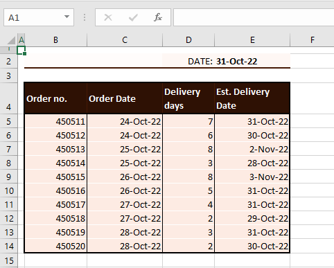
Let’s use an example to better explain the works. In our example case, the current date is the 31^st of October 2022. The date has been entered in cell E2. We have a list of customer orders with the order date, delivery days, and estimated delivery date mentioned. As the deliveries are completed, the orders are cleared from this list.

The objective is to find which orders have deliveries overdue so that they can be tended to quickly. Now is where the formulas come in and do their job.

Using Generic Formula

Checking if a date falls before today can be done without delving into anything technical. You can use a simple formula where you check if the date is less than the date today. And… job done! Let’s put the no-nonsense formula to the test. Use a formula like the one below to check if today’s date comes after a date:

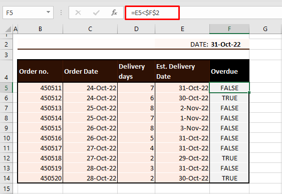
=E5<$F$2

With this formula, we are checking if the date in E5 i.e. 31-Oct-22 occurs before the date in F2 which is 31-Oct-22. The «before» bit of the formula is checked with the less than sign, meaning is E5’s date less than F2’s date? Since both the dates are the same and one is not less than the other, the formula returns FALSE.

In the next instance, we will be checking E6 against F2. F2 remains constant against the dates in column E because it has been locked as an absolute reference with $ signs. 30-Oct-22 is lesser than the 31^st so we get a TRUE this time. This means that the date in E6 is before the current date entered in F2. So on, and so forth, we get the F column filled with this formula:

Nice going. But we need better going. Wouldn’t it be better to have something a little more prominent than TRUE and FALSE stacked up? It would indeed. Let’s see what we can do about that.

Using TODAY Function

We can check a date against the current date with help from the TODAY function. The TODAY function returns the current date in the default date format. We can have a little demonstration before we proceed to the actual objective.

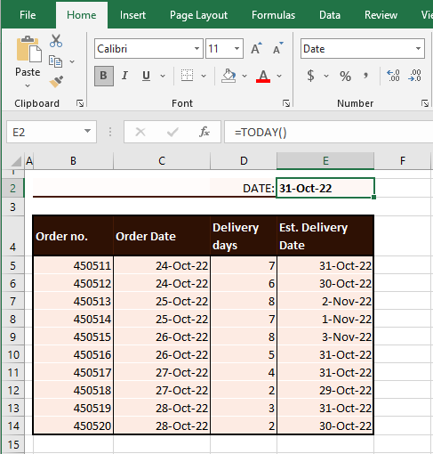
In our case example, we will enter today’s date using the TODAY function instead of manually punching it in. We have entered this date with the TODAY function without any arguments and we get 31-Oct-22 as the result:

In this circumstance, you can still resort to the formula used above i.e. =E5<$F$2

Now if we were to use the formula plainly as we did earlier, we’d use the logical test as:

=E5<TODAY()

But that would give us TRUEs and FALSEs again. So let’s have the formula that we will be working with to check the current date against the dates in column E, to see if they are before or after the 31^st. Using the TODAY and IF functions, we get:

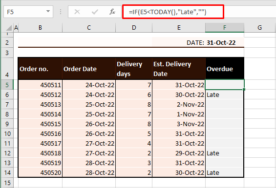
=IF(E5<TODAY(),"Late","")

The logical test that we were going to use on its own has been nested in the IF function. The IF function will check if E5’s date is less than (and therefore earlier than) the date today (supplied by the TODAY function). We know the answer to that is FALSE.

Upon returning TRUE, the IF function is set to return the text string «Late» (as has been done in the second instance). For FALSE the result is to be an empty text string (denoted by a pair of double quotes «») as returned in F5:

If you’ve figured out the plus point of integrating the TODAY function, 10 points to you. The plus is that TODAY will have dynamic results; updating column F as the date changes. Taking the example of our case, the next day, on the 1^st of November, the results will be «Late» for F5 – F6 and F10 – 14.

That is because all these dates will fall before the 1^st of November. To keep the results on your worksheet static, skip using the TODAY function and stick to a generic formula like in the previous section.

Working with Missing Dates

Incorporating other factors into the mix, suppose we have some estimated delivery dates missing as the delivery dates of some orders are unknown. With missing dates, either of the formulas from above would equate to TRUE, as a missing date can’t be said to not be before the current date.

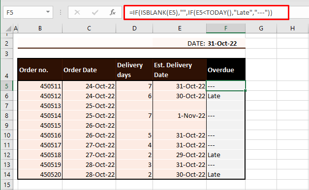
This would be a little misleading, and the fix for this mix is the ISBLANK function. The formula below will help you to check if a date comes before the current date while dealing with missing dates:

=IF(ISBLANK(E5),"",IF(E5<TODAY(),"Late","---"))

Now we have geared up the formula to return an empty text string «» upon finding a blank cell in column E, indicating a missing date. If not, meaning if a date is found, then the date should be tested for falling before today’s date (as provided by the TODAY function). If yes, then we get «Late», or else we get «—».

Using Conditional Formatting

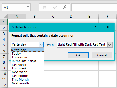
The second major way is using Conditional Formatting to check if the current date is before or after another date. Conditional Formatting is a very visual method of highlighting data that meets a certain condition in Excel. The A Date Occurring rule in Conditional Formatting provides a few earlier date options:

Using these preset options can highlight yesterday’s date or dates having occurred in the last 7 days, last week, or last month.

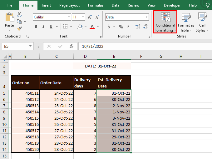
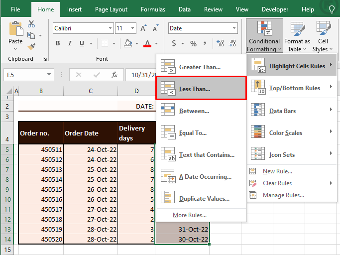
We will aim to highlight those dates in Excel that precede today’s date by a Conditional Formatting rule. Go through the steps below to see the rule we’re applying through Conditional Formatting to check if a date is before the current date:

• Select the cells with the dates that you want to check against today’s date.
• Select the Conditional Formatting icon from the Styles group in the Home

• From the menu, go to Highlight Cells Rules > Less Than.

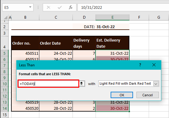
• In the opened dialog box, type the following formula:

=TODAY()

• Use the next bar to set the format for the highlighted cells.

• The background of this rule is what we have seen in the earlier sections; checking the date to be less than the date today. From the selected cells, Conditional Formatting will highlight all the cells meeting this condition in Light Red Fill with Dark Red Text.
• Click on the OK button in the dialog box.

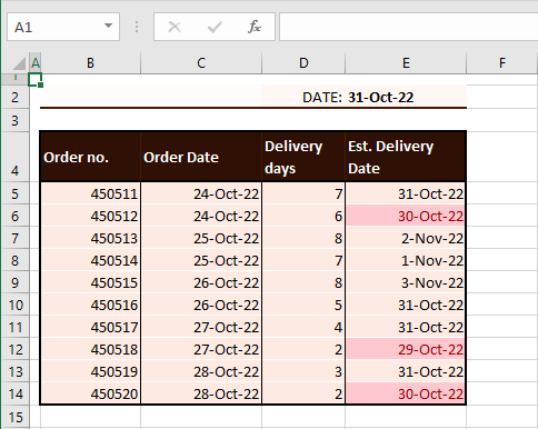
The dates falling before the 31^st of October will be highlighted:

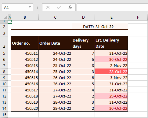
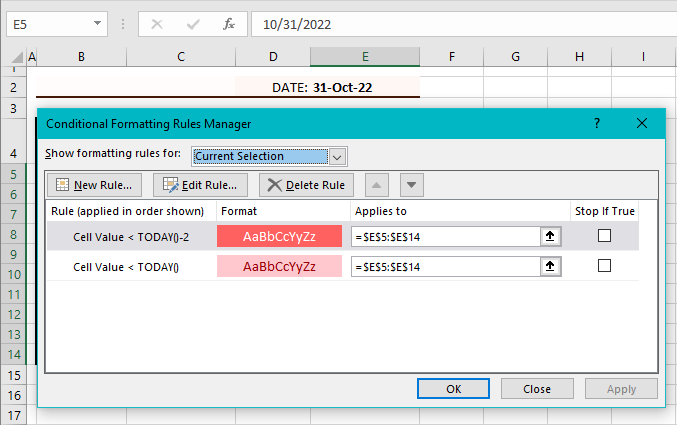
Let’s tweak the data a bit so that along with these highlighted 3 dates, we’ll have the date 28^th October which will be the date furthest behind the 31^st in the dataset. Leaving the previous Conditional Formatting rule as it is, 28^th will then also be highlighted in light red. If we add another rule similar to the previous one, the only change is in the TODAY function as follows:

=TODAY()-2

This will highlight the dates less than 2 days from today and we’ve chosen red fill so it further stands out:

All days that are two or more days before today will be highlighted in red fill. However, make sure to keep the second rule in top preference otherwise the dates will only fall under the first rule. The preference can be changed in the Conditional Formatting Rules Manager.

This was how to use the TODAY function to highlight dates more than x days before the current date. E.g. highlighting the dates more than 2 weeks before the current date can be done with the Less Than rule with the following input formula:

=TODAY()-14

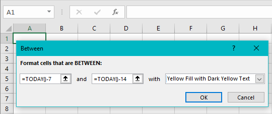
With the Between Highlight Cells rule, Conditional Formatting can highlight the dates occurring, let’s say, between 2 weeks to a week before today like so:

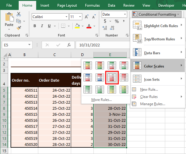
Conditional Formatting provides a very easily deducible visual, right? The longer dues in a darker shade. You can leave that all to Excel and set this up in a matter of seconds with Conditional Formatting‘s Color Scales option. To apply it, go to the Home tab > Conditional Formatting icon > Color Scales and choose a Color Scale. We’ve chosen a 2-Color Scale.

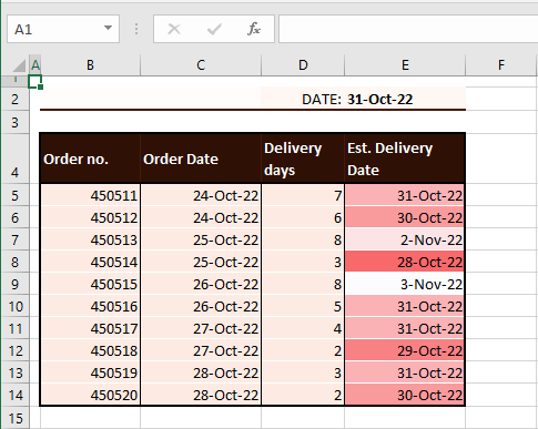
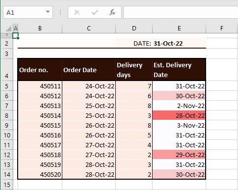
The Color Scale will be applied immediately highlighting the earliest date in red and shading the dates as per the Color Scale tones to the latest date in white.

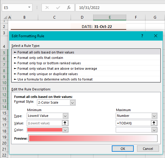
While this is cool, it’s missing the TODAY component. We have a little trick to make this Color Scale relevant to the date today so head to the Rule Manager and edit the rule involving this Color Scale.

On the Maximum side that is represented by the white color, change the Type to Number. In the Value field, enter the TODAY function as:

=TODAY()

The purpose of these changes is to limit the Color Scale to just the current date instead of the latest date in the selected cells. Apply the changes with the OK command.

See the change in the Conditional Formatting? Now only the dates before the current date are prominent while the current date and beyond are white.

And here’s where we check out. That was our tutorial with some easy tricks on checking if a date is before today’s date in Excel where the TODAY function can play a very convenient role. While you’re getting your way around with dates, we’ll work on more Excel matter for your checking.

Checking for dates in Excel can be a very interesting problem as Excel stores dates as numbers. For example, 4-Jul-15 is stored as 42189.

To elaborate further on this, 1-Jan-1900 is treated as 1. The difference between a date and 1-Jan-1900 +1 is the serial number of that date. hence, in case of 4-Jul-15, it is 42189.

Hence, if you write 42189 and 4-Jul-15 in two different cells, Excel has no built-in mechanism to differentiate between these two.

Excel can not tell whether the written value is a date or not. All the date operations which you can do with 4-Jul-15, you can do with 42189 also.

There are many possible workarounds but none of them are perfect. The only way is to use VBA for this. Don’t get intimidated by VBA. This is fairly simple, only 3 lines of codes. Just follow the below steps –

1. ALT+F11 to open VBA Window.

2. Look on left side, there is Project Explorer Window. Locate your workbook name. Workbook name will be in parenthesis and preceded by word VBA project.

3. You may have modules already in your VBA Project. But I am presuming, you will have none as this article is mostly for non-VBA types. Irrespective of the fact, whether module is there or not, follow next step.

4. Right Click on your VBA Project > Insert > Module

5. If there is something existing in your Module, remove it.

6. Copy and Paste following 3 lines in your module –

Function IsDate(cell) As Boolean
IsDate = VBA.IsDate(cell)
End Function

7. Now, you can simply say =ISDATE(A1) if your date is in A1 in your workbook in any worksheet and if the cell is date, you will get TRUE otherwise, you will get FALSE.

NOTE – You will have to save your workbook as .xlsm to use the above function.