
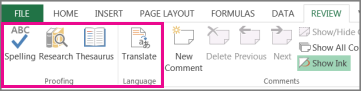
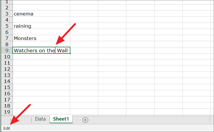
To check spelling for any text on your worksheet, click Review > Spelling.
Tip: You can also press F7.
Here are some things that happen when you use the spelling checker:
-
If you select a single cell for spell check, Excel checks the entire worksheet, including the comments, page headers, footers and graphics.
-
If you select multiple cells, Excel checks spelling only for those cells.
-
To spell check words in a formula bar, select the words.
Note: Excel doesn’t check spelling in cells that contain formulas.
Correct spelling as you type
Both AutoComplete and AutoCorrect can help fix typing errors on the go.
AutoComplete, on by default, helps to maintain accuracy as you type by matching entries in other cells and does not check individual words in a cell, AutoComplete can be handy when creating formulas.
AutoCorrect fixes errors in a formula’s text, worksheet control, text box, and chart labels. Here’s how to use it:
-
Click File > Options.
-
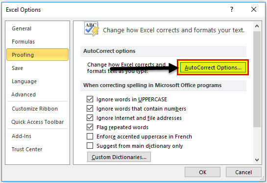
Under the Proofing category, click AutoCorrect Options, and check the most likely typing errors.
Note: You can’t use AutoCorrect for text in a dialog box.
Additional resources
You can also check out Research, Thesaurus and Translate for more help with spelling and language.
-
On the Review tab, click Spelling or press F7 on the keyboard.
Note: The Spelling dialog box will not open if no spelling errors are detected, or if the word you are trying to add already exists in the dictionary.
-
Do any of the following.
To
Do this
Change the word
Under Suggestions, click the word that you want to use, and then click Change.
Change every occurrence of this word in this document
Under Suggestions, click the word that you want to use, and then click Change All.
Ignore this word and move on to the next misspelled word
Click Ignore.
Ignore every occurrence of this word in this document and move on to the next misspelled word
Click Ignore All.
Correct spelling as you type
You can use the AutoCorrect feature to correct typos and misspelled words. For more information, see Add, edit, or turn off automatic corrections.
To check spelling for any text on your worksheet, click Review > Proofing > Spelling.
Imagine preparing high-profile reports and being the sole creator of a greatly discreditable spelling error in one of the headers. Huff times hundred! We suppose that is enough to make you realize the necessity of checking spellings in Excel because, unlike MS Word, you will not see any red squiggly underlines that will prompt you to fix misspellings. So really, spell check is your best bet!
Although we have AutoCorrect to save face in some prearranged spelling situations, there’s only so much AutoCorrect can do and you will need the helping hand of a spelling check. Spell check is a sub-feature of proofing in Excel. It gives the user the option to deal with incorrect spellings, typos, and a consecutively repeated word. Note that spell check does not take care of grammatical errors.

Today’s tutorial will give you the chance to learn everything about spell check in Excel. You’ll discover what spell check can do, how to spell check (where you will find spell check itself and its options, the shortcut key, using VBA for spell checking), what you can spell check (cell(s), part of a cell, sheet(s)), how to tweak spell check, and where you are going wrong if spell check isn’t working.
Without further ado, Madam Excel, correction pen at the ready!
Recommended Reading: Excel AutoCorrect Feature -Detailed Guide
How to Spell Check in Excel
In the Ribbon menu, the spell check option is accessible from the Review tab. To use spell check, you need to select the relevant cell(s) or sheet(s). Ahead in the tutorial, we’ll show you what selecting certain cells or sheets will do when you run spell check.
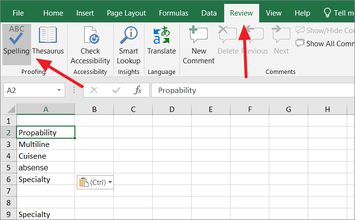
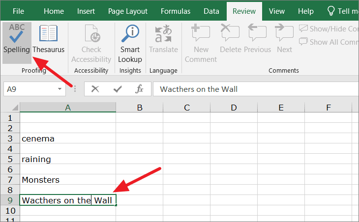
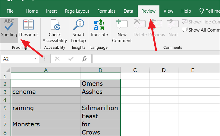
For now, let’s see how to start spell check. Go to the Review tab and select the Spelling button from the Proofing group in the tab.

Now the Spelling window will open and this will be used to check the spellings on the worksheet. This is the window you will see:

Keyboard Shortcut for Spell Checking
Alternatively, spell check can also be quickly run by a keyboard shortcut. In fact, in this case, it’s just one shortcut key.
Press the F7 key to run spell check in Excel.
The F7 key will do the same work as using the Spelling button from the Ribbon and will launch the Spelling window as shown above.
How Does Spell Check Work
Now how does spell check go about its spell-checking. Spell check starts checking from the cell in selection and goes row by row. This means that spell check works from left to right, then downward, and left to right again.
Spell check automatically jumps from the cell in selection to the cell with the spelling error. So if there’s any cell in between the initially selected cell and the cell being checked by spell check that you reckoned needed attention, spell check has ignored it. Later, you will find out what type of data is ignored by spell check.
Now allow us to demonstrate the works of spell check. In the example shot below, we have selected the first cell of the sheet i.e. cell A1.

Now when spell check is run from the Ribbon or by pressing F7, spell check begins checking each cell starting from the cell in selection (A1 in this case). The feature goes row by row checking A1, B1, C1, and so forth until every cell in row 1 is checked. Then it starts with row 2, checking A2, B2, C2, so forth.
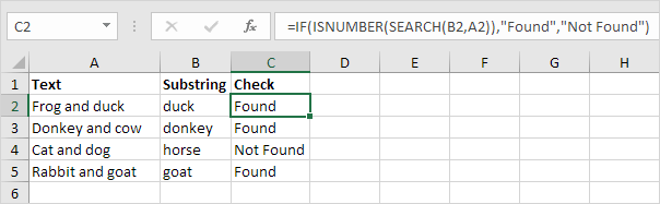
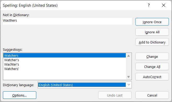
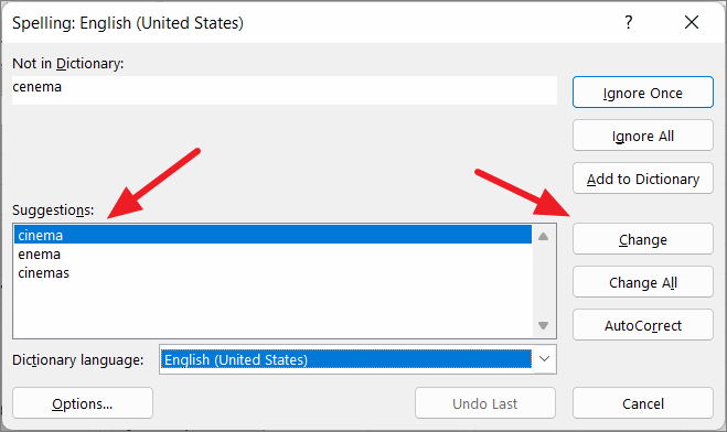
In our example case, the first non-empty cell is B2. Every cell is checked rightward for spelling and the first cell that has been found with a spelling error is C4. C4 has two incorrect spellings hence, spell check starts working on the first word i.e. Hppy in the Spelling dialog box:

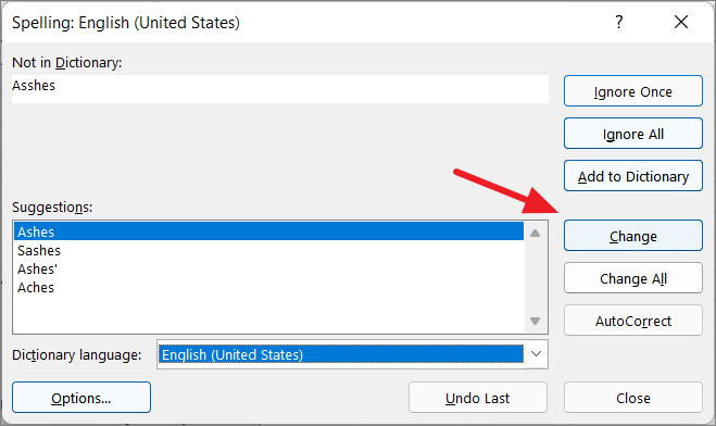
Once the word has been dealt with by the user by ignoring or changing it, spell check will present the next spelling error in the same cell if any. C4 in our case example contains a second incorrect spelling which is presented next in the Spelling dialog box:

After spell check has tended to each incorrectly spelled word one by one in the cell, it moves to the next cell with spelling errors. Checking the cells rightward and then downward, spell check found the next spelling error in C5:

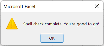
This is how spell check will work word by word and cell by cell to present all the spelling errors and what to do about them in the Spelling dialog box. When spell check has checked every occupied cell on the worksheet, a small window will pop up confirming that the spell check has been completed:

If Excel says you’re good to go, you most probably are! Press the OK command to close the pop-up and return to the worksheet.
Important question. How does spell check know what word to pick on? Spell check will go for the words that aren’t enlisted in Excel’s main and custom dictionary.
Understanding the Spell Check Window Options
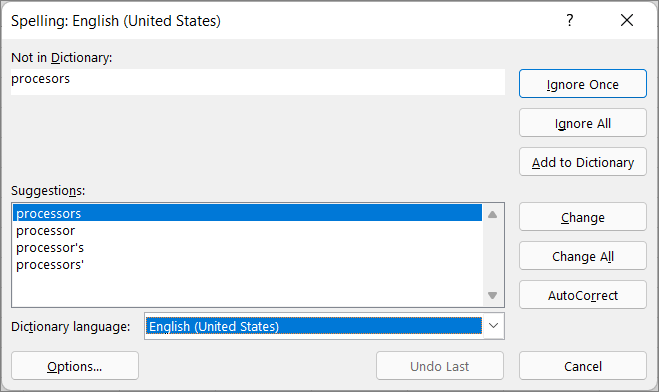
We just went through how spell check works and that’s something it does on its own. What control do you have over spell check? Now we’ll run you through the options in the Spelling window so we know what can be done with the spelling errors. Let’s have a look at the Spelling window again:

Not in Dictionary
The word with incorrect spelling that has been detected by spell check will show in the Not in Dictionary field. You can manually edit the spelling by clicking on the text box but take a look at the Suggestions section first.
Suggestions
Here you will find the word(s) suggested by Excel as corrections.
Command Buttons:
- Ignore Once – The shown word will not be corrected and spell check will ignore it and move on to the next incorrect spelling. If the misspelling is deliberate, you can use this button to skip to the next incorrectly spelled word.
- Ignore All – If the same misspelling is present more than once in the spell check region, they will all be ignored if you click on this button.
- Add to Dictionary – This button will add the misspelled word to the custom dictionary. By doing this, you will prevent the misspelling from showing up in the current and future spell checks.
- Change – This is the most important button in the window (you wouldn’t be using spell check if you didn’t want to correct anything). Before using this button, you need to select the word from the Suggestions section that you want as the replacement for the misspelled word. Next, you will select the Change button to complete the action of correcting the misspelled word.
- Change All- Similar to how the Ignore All button works. If there is a repetition of the misspelled word in the spell check region, using this button will change all of them as per the word selected in the Suggestions section.
- AutoCorrect – The AutoCorrect button will add the misspelled word and its replacement selected from the Suggestions section to the AutoCorrect list. This button works prospectively. E.g. the misspelled word was “hppy” and the replacement word chosen from Suggestions was “happy”. The next time “hppy” is entered in Excel, it will automatically be corrected to “happy”.
- Options – The Options button leads to the spelling settings in Excel Options. We will talk about these options later on.

- Undo Last – With this button, you can undo the last correction. The change will be reversed and spell check will go back to the misspelled word in the Spelling window. This should be helpful if you’ve accidentally selected the wrong word in Suggestions. By undoing the correction, you can go back and select the right word.
- Cancel – This will close the Spelling window and abort the spell check operation even if there are misspelled words left to be tended to.
Spell Check Scope
Now we explore the extent of spell check; what it can check. It is particularly helpful to know the reach of spell check so you can check as little or as much as you require. Below we have the details to test as less as part of a cell and as much as the entire workbook for spelling.
Individual Cells and Ranges
This section covers spell checking scope on the active worksheet.
Part of cell
To only check part of a cell for incorrect spellings, go in cell edit mode by double clicking the target cell or selecting the cell and using the Formula Bar. Then select the relevant text.
Now you can select the Spelling button from the Review tab or press F7 to spell-check the selected part of the cell.

A single cell
To spell check the entire contents of just one cell, after entering cell edit mode of the target cell, select the entire contents of the cell. Then run spell check.

Range of cells
To spell check a certain range of cells, select the range(s) and hit spell check.

Spell check will also work for disjoined ranges selected by holding down the Ctrl key.
Continuous part of worksheet ‘til the end
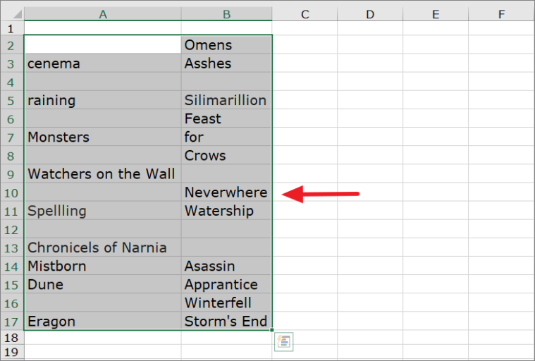
If you select a certain cell and run spell check, it will cover the selected cell down to the last non-empty cell on the worksheet. This means that the sheet will be spell-checked from the selected cell until the end of the worksheet. E.g. in our example shot below, we have selected C5.

If we run spell check right now, the cells that will be covered are C5 to the end of the worksheet (i.e. up to the last occupied cell, which is C11).
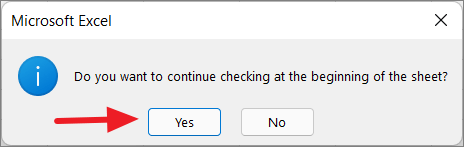
Once the spell check is completed to C11, since the worksheet hasn’t been checked from the start, you will see a small dialog box asking if you want to check the sheet from the beginning:

Excel is mindful that you might not be good to go yet… If you now choose to have the sheet checked from the beginning, the checking will end at C4 (i.e. up to the selected cell).
Entire worksheet
To have the full worksheet checked for spellings, select the first cell of the sheet i.e. A1 and run the spell check using the F7 key.

According to the checking properties mentioned above, the sheet will be checked from the selected cell to the end so that effectively tests the entire worksheet.
Selected Sheets
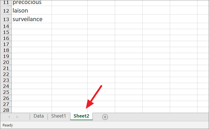
Spell check can cover multiple sheets at a time too if they are selected. To select the target sheets, keep the Ctrl key pressed and click on the sheet tabs above the status bar.

Now run spell check to test the selected sheets for misspelled words. You can select discontinuous sheets too, e.g sheets 2 and 5.
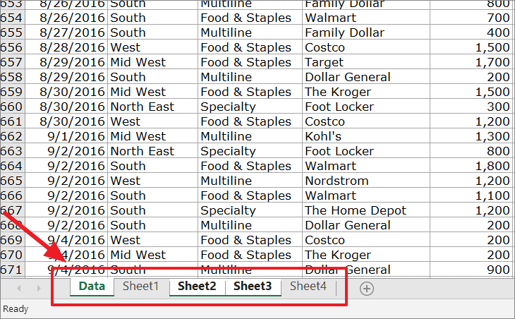
Entire Workbook
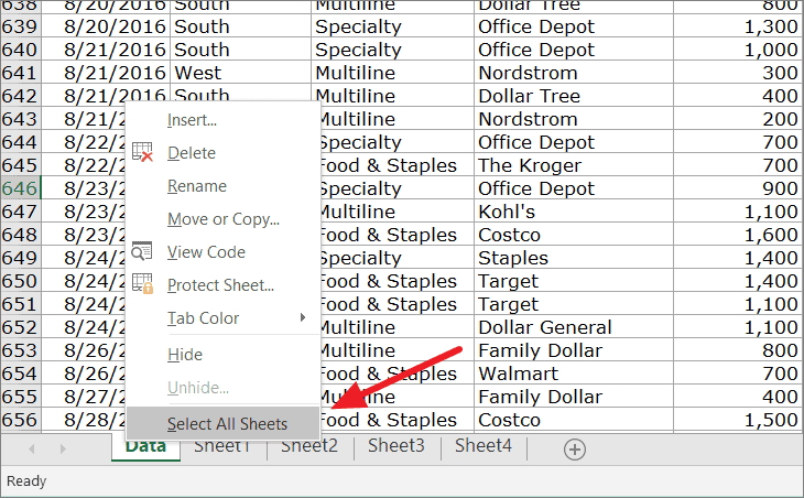
For checking the whole workbook with spell check, you need to select all the sheet tabs at the bottom. The quick way to do that is to right-click any sheet tab and select the option Select All Sheets from the menu.

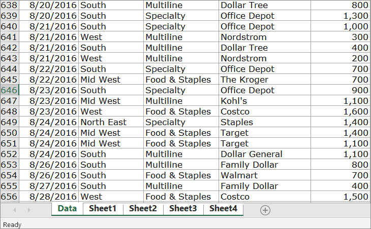
This option will select all the sheets in the workbook:

Now once all the sheets are selected hit the F7 key to run the spell check for entire workbook.
Tip: If you want to select all the sheets except one, you can use the shortcut above to select all the sheets and then press the Ctrl key and click on the sheet you don’t want checked for spelling. That will exclude the unselected sheet.
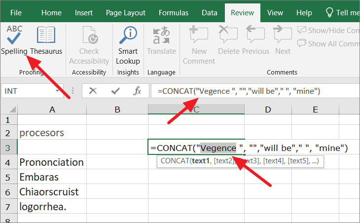
Text in Formulas
Checking the text in formulas applies the same way as checking the text of an entire cell because that is essentially what you’ll be doing. Why you need to check the formula specifically is because formula cells will be ignored by spell check.
Start edit mode of the cell (using F2 key) with the formula and select the contents of the cell (and therefore the complete formula):

After selecting the formula, run spell check to pick out the misspellings.
Spell Check Settings In Excel
Remember we said we’ll discuss the spell check options? Now’s the time. By default, spell check will ignore certain kinds of text and flag the other kinds. The spell check settings we will show you ahead give you a bit more control on how spell check will work. Before we talk about these settings, let’s see how to reach them:
Excel Options are accessible from the File tab:

The complete path is File tab > Options > Proofing tab. But the shortcut path is the one we showed you earlier.
- Launch the Spelling window by the F7 key or from the Review
- In the window, select the Options

This will also lead to the Proofing tab in Excel Options.

The highlighted section is our point of interest. The options in the example shot above are the default settings. Let’s talk about these options now.
Ignore words in UPPERCASE
It’s a good idea to leave this option checked since some words will need to be used in complete uppercase letters but do bear in mind that if a word is in uppercase and is misspelled, it’ll still be ignored in spell check.
The following text will be overlooked by spell check: EXCELTRICK
Ignore words that contain numbers
Mixed text can be a part of codes e.g product codes.
This text will be ignored by spell check: AE0158
Ignore Internet and file addresses
Network and file paths will not be checked for spelling.
The following addresses will not be selected in spell check: www.exceltrick.com or C:exceltrick
Flag repeated words
Repetition of the same word will be flagged.
In the following text, the second “here” will be flagged by spell check: Enter here here
Enforce accented uppercase in French
This option is concerned with working in French (Canada) in Excel and when this option is checked, it can flag unaccented French uppercase.
The word “Elan” will be detected by spell check and suggested to be changed to “Élan”.
Suggest from main dictionary only
If you want spell check to ignore the entries in the custom dictionary, check this option.
Other options
The Custom Dictionaries button leads to, of course, custom dictionaries:

Here, you can create dictionaries for whichever language you want to use in Excel and it will only apply to that particular language. You can also edit the word list of the All Languages dictionary. Entries in this dictionary will apply to all languages.
The other two options in the Excel Options window include a few controls of language options regarding French and Spanish.
The last option gives the user choice to change the dictionary language.
Spell Check Not Working
There are many instances when Excel doesn’t behave the way we want it to and a few of those occurrences fall under spell check. Find out why spell check doesn’t work at times and what are the solutions.
Spell Check Button Disabled
If the Spelling button in the Ribbon is disabled (grayed out) you also won’t be able to use the shortcut key F7. This is likely to happen if the worksheet is protected. If you wish to run spell check, unprotect the sheet first by going to the Review tab > Protect group > Unprotect Sheet button.

Once the sheet is unprotected, the Spelling button will be enabled again:

Formula Cells not Checked
As mentioned earlier on, formula cells will go disregarded by spell check. Formulas will have to be checked individually by selecting the entire contents of the formula cell and running spell check on it.
Spell Check only Working for Active Cell
It may so happen that spell check is only working for one cell. In that case, you may accidentally be in cell edit mode and hence spell check is only running for the active cell. Exit editing the cell to make spell check work for the sheet.
Spell Check Using VBA
The spellings in Excel can be checked using VBA. VBA is a Microsoft programming language that efficiently systemizes carrying out repetitive tasks. The task will be carried out by running a specific code. The detailed steps to run the code using VBA are listed as follows:
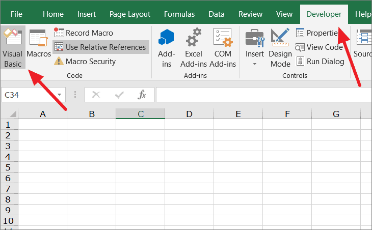
- To launch the VB editor, press the Alt + F11 You can also use the Developer tab if it is enabled on your Excel. In the Developer tab, select the Visual Basic button from the Code group.

- Here enters the VB editor:

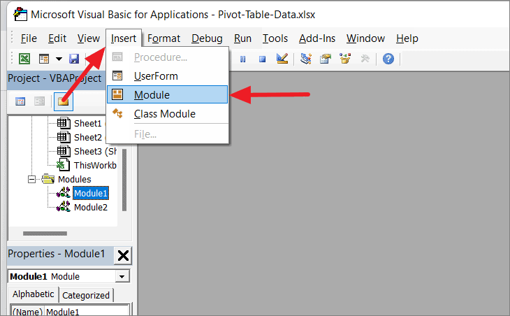
- Use the Insert tab to launch a Module window by selecting Module from the menu.

- Now you will see a Module window:

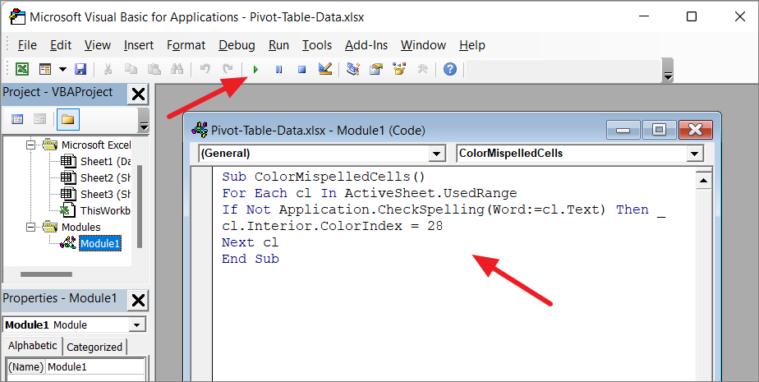
- Copy the code below and paste it into the Module window:
Sub SpellCheckActiveSheet()
 ActiveSheet.CheckSpelling
End Sub
The code activates spell check for the active worksheet.

The code can be run later. To do that, you will have to close the VB editor as the Macro is already created. Then you can run the code from the View or Developer tab’s Macro button or by pressing the Alt + F8 keys to select the related Macro.
- To run the code instantly from the Module window after pasting the code, select the Run button from the toolbar.

Running the code opens the Spelling window and spell check gets down to work!

Once the spell check is done, you will be redirected to the Module window if you had run the code from there. You may close the VB editor now.
Note: Regardless of the cell selection on the sheet, the code given above will spell check the entire worksheet.
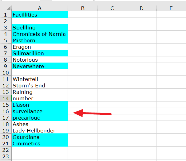
Highlight Misspelled words In Active Sheet Using VBA
Following VBA code changes the background color of the cells where misspelled words are present. This makes it easier for anyone to find the wrongly spelled words just by looking at the sheet.
Sub ColorMispelledCells()
For Each cl In ActiveSheet.UsedRange
 If Not Application.CheckSpelling(Word:=cl.Text) Then _
 cl.Interior.ColorIndex = 28
Next cl
End Sub
Spell-Checking Visible Sheets Using VBA
If there are any hidden sheets in your workbook and you want to leave them out of spell check, use the code below in VBA:
Sub SpellCheckAllVisibleSheets()
For Each wks In ActiveWorkbook.Worksheets
 If wks.Visible = True Then
 wks.Activate
 wks.CheckSpelling
 End If
Next wks
End Sub
Spell-Checking Visible and Hidden Sheets Using VBA
This code will spell check all the sheets in the workbook; hidden and visible.
Sub SpellCheckAllSheets()
For Each wks In ActiveWorkbook.Worksheets
 wks.CheckSpelling
Next wks
End Sub
While running this code, the current sheet will remain in selection and spell check will not snap to each sheet that is being spell-checked (because how can spell check snap to a hidden sheet, right?
Right! That was a full-blown rollercoaster ride on spell check in Excel. We cracked every motor down and oiled every machine well. To make sure every Excel ride is as smooth as this one, we’ll tune out for now but you be ready to tune in shortly!
Содержание
- Check if a cell contains text (case-insensitive)
- Find cells that contain text
- Check if a cell has any text in it
- Check if a cell matches specific text
- Check if part of a cell matches specific text
- Contains Specific Text
- How to spell check in Excel
- How to do spell check in Excel
- Spell check individual cells and ranges
- How to check spelling in multiple sheets
- How to spell check the entire workbook
- How to spell check text in formulas
- Spell check in Excel using a macro
- Macro to do spell check in the active sheet
- Macro to spell check all sheets of the active workbook
- Highlight misspelled words in Excel
- How to use spell checking macros
- Change the Excel spell check settings
- Excel spell check not working
- Spelling button is greyed out
- You are in edit mode
- Text in formulas is not checked
- Find typos and misprints with Fuzzy Duplicate Finder
Check if a cell contains text (case-insensitive)
Let’s say you want to ensure that a column contains text, not numbers. Or, perhapsyou want to find all orders that correspond to a specific salesperson. If you have no concern for upper- or lowercase text, there are several ways to check if a cell contains text.
You can also use a filter to find text. For more information, see Filter data.
Find cells that contain text
Follow these steps to locate cells containing specific text:
Select the range of cells that you want to search.
To search the entire worksheet, click any cell.
On the Home tab, in the Editing group, click Find & Select, and then click Find.
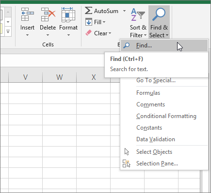
In the Find what box, enter the text—or numbers—that you need to find. Or, choose a recent search from the Find what drop-down box.
Note: You can use wildcard characters in your search criteria.
To specify a format for your search, click Format and make your selections in the Find Format popup window.
Click Options to further define your search. For example, you can search for all of the cells that contain the same kind of data, such as formulas.
In the Within box, you can select Sheet or Workbook to search a worksheet or an entire workbook.
Click Find All or Find Next.
Find All lists every occurrence of the item that you need to find, and allows you to make a cell active by selecting a specific occurrence. You can sort the results of a Find All search by clicking a header.
Note: To cancel a search in progress, press ESC.
Check if a cell has any text in it
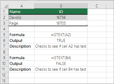
To do this task, use the ISTEXT function.
Check if a cell matches specific text
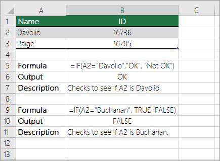
Use the IF function to return results for the condition that you specify.
Check if part of a cell matches specific text
To do this task, use the IF, SEARCH, and ISNUMBER functions.
Note: The SEARCH function is case-insensitive.
Источник
Contains Specific Text
To check if a cell contains specific text, use ISNUMBER and SEARCH in Excel. There’s no CONTAINS function in Excel.
1. To find the position of a substring in a text string, use the SEARCH function.
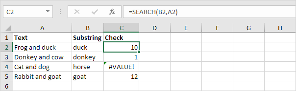
Explanation: «duck» found at position 10, «donkey» found at position 1, cell A4 does not contain the word «horse» and «goat» found at position 12.
2. Add the ISNUMBER function. The ISNUMBER function returns TRUE if a cell contains a number, and FALSE if not.
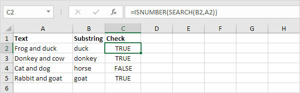
Explanation: cell A2 contains the word «duck», cell A3 contains the word «donkey», cell A4 does not contain the word «horse» and cell A5 contains the word «goat».
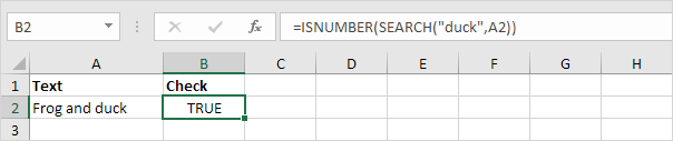
3. You can also check if a cell contains specific text, without displaying the substring. Make sure to enclose the substring in double quotation marks.
4. To perform a case-sensitive search, replace the SEARCH function with the FIND function.
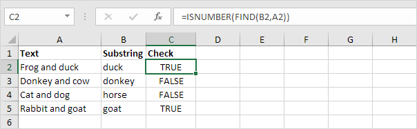
Explanation: the formula in cell C3 returns FALSE now. Cell A3 does not contain the word «donkey» but contains the word «Donkey».
5. Add the IF function. The formula below (case-insensitive) returns «Found» if a cell contains specific text, and «Not Found» if not.
6. You can also use IF and COUNTIF in Excel to check if a cell contains specific text. However, the COUNTIF function is always case-insensitive.

Explanation: the formula in cell C2 reduces to =IF(COUNTIF(A2,»*duck*»),»Found»,»Not Found»). An asterisk (*) matches a series of zero or more characters. Visit our page about the COUNTIF function to learn all you need to know about this powerful function.
Источник
How to spell check in Excel
 by Svetlana Cheusheva, updated on March 16, 2023
The tutorial shows how to perform spell check in Excel manually, with VBA code, and by using a special tool. You will learn how to check spelling in individual cells and ranges, active worksheet and the entire workbook.
Although Microsoft Excel is not a word processing program, it does have a few features to work with text, including the spell-checking facility. However, spell check in Excel is not exactly the same as in Word. It does not offer advanced capabilities like grammar checking, nor does it underline the misspelled words as you type. But still Excel provides the basic spell checking functionality and this tutorial will teach you how to get most of it.
How to do spell check in Excel
No matter which version you are using, Excel 2016, Excel 2013, Excel 2010 or lower, there are 2 ways to spell check in Excel: a ribbon button and a keyboard shortcut.
Simply, select the first cell or the cell from which you’d like to start checking, and do one of the following:
- Press the F7 key on your keyboard.
- Click the Spelling button on the Review tab, in the Proofing group.
This will perform a spelling check on the active worksheet: 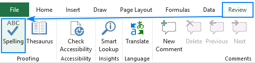
When a mistake is found, the Spelling dialog window shows up: 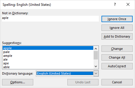
To correct a mistake, choose an appropriate opting under Suggestions, and click the Change button. The misspelt word will be replaced with the selected one and the next mistake will be brought to your attention.
If the «mistake» is not really a mistake, pick one of the following options:
- To ignore the current mistake, click Ignore Once.
- To ignore all the mistakes same as the current one, click Ignore All.
- To add the current word to dictionary, click Add to Dictionary. This will ensure that the same word won’t be treated as a mistake when you do a spell check next time.
- To replace all the mistakes same as the current one with the selected suggestion, click Change All.
- To let Excel correct the mistake as it sees fit, click AutoCorrect.
- To set another proofing language, select it from the Dictionary language drop box.
- To view or change the spell check settings, click the Options… button.
- To stop the correction process and close the dialog, click the Cancel button.
When the spell check is complete, Excel will show you the corresponding message: 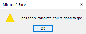
Spell check individual cells and ranges
Depending on your selection, Excel Spell check processes different areas of the worksheet:
By selecting a single cell, you tell Excel to perform spell check on the active sheet, including text in the page header, footer, comments, and graphics. The selected cell is the starting point:
- If you select the first cell (A1), the entire sheet is checked.
- If you select some other cell, Excel will start spell checking from that cell onward till the end of the worksheet. When the last cell is checked, you will be prompted to continue checking at the beginning of the sheet.
To spell check one particular cell, double-click that cell to enter the edit mode, and then initiate spell check.
To check spelling in a range of cells, select that range and then run the spell-checker.
To check only part of the cell contents, click the cell and select the text to check in the formula bar, or double click the cell and select the text in the cell.
How to check spelling in multiple sheets
To check several worksheets for spelling mistakes at a time, do the following:
- Select the sheet tabs you wish to check. For this, press and hold the Ctrl key while clicking the tabs.
- Press the spell check shortcut ( F7 ) or click the Spelling button on the Review tab.
Excel will check spelling mistakes in all the selected worksheets: 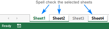
When the spell check is completed, right click the selected tabs and click Ungroup sheets.
How to spell check the entire workbook
To check spelling in all the sheets of the current workbook, right click on any sheet tab and pick Select all Sheets from the context menu. With all the sheets selected, press F7 or click the Spelling button on the ribbon. Yep, it’s that easy! 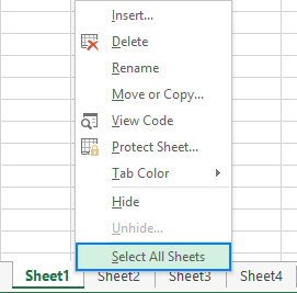
How to spell check text in formulas
Normally, Excel does not check formula-driven text because a cell actually contains a formula, not a text value: 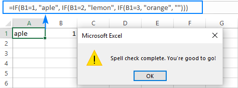
However, if you get in the edit mode and then run spell check, it will work: 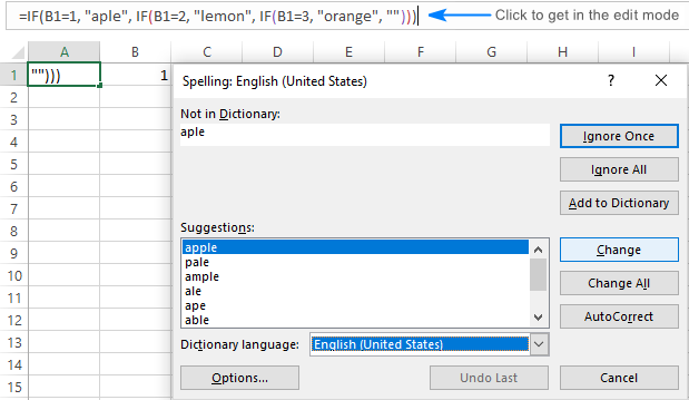
Of course, you will need to check each cell individually, which is not very good, but still this approach may help you eliminate spelling errors in big formulas, for example, in multi-level nested IF statements.
Spell check in Excel using a macro
If you like automating things, you can easily automate the process of finding wrongly spelled words in your worksheets.
Macro to do spell check in the active sheet
What can be simpler than a button click? Maybe, this line of code 🙂
Macro to spell check all sheets of the active workbook
You already know that to search for spelling mistakes in multiple sheets, you select the corresponding sheet tabs. But how do you check hidden sheets?
Depending on your target, use one of the following macros.
To check all visible sheets:
To check all sheets in the active workbook, visible and hidden:
Highlight misspelled words in Excel
This macro allows you to find the misspelled words simply by viewing the sheet. It highlights the cells containing one or more spelling mistakes in red. To use another background color, change the RGB code in this line: cell.Interior.Color = RGB(255, 0, 0).
How to use spell checking macros
Download our sample workbook with Spell Check macros, and perform these steps:
- Open the downloaded workbook and enable the macros if prompted.
- Open your own workbook and switch to the worksheet you want to check.
- Press Alt + F8 , select the macro, and click Run.
The sample workbook contains the following macros:
- SpellCheckActiveSheet — performs a spell check in the active worksheet.
- SpellCheckAllVisibleSheets — checks all visible sheets in the active workbook.
- SpellCheckAllSheets — checks visible and invisible sheets in the active workbook.
- HighlightMispelledCells — changes the background color of cells that contain wrongly spelled words.
You can also add the macros to you own sheet by following these instructions: How to insert and run VBA code in Excel.
For example, to highlight all the cells with spelling errors in the current spreadsheet, run this macro: 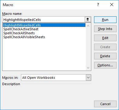
And get the following result: 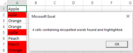
Change the Excel spell check settings
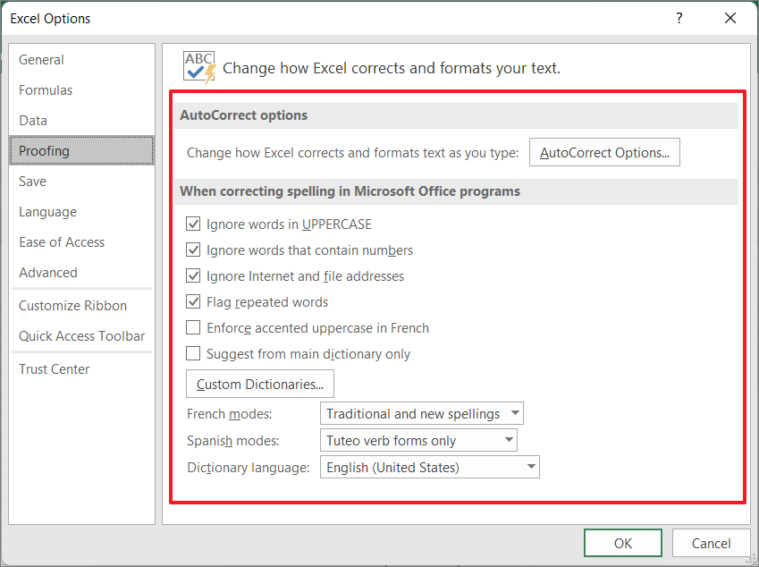
If you’d like to tweak the behavior of spell check in Excel, click File > Options > Proofing, and then check or uncheck the following options:
- Ignore words in uppercase
- Ignore words that contain numbers
- Ignore internet files and addresses
- Flag repeated words
All the options are self-explanatory, maybe except the language-specific ones (I can explain about enforcing strict ё in the Russian language if someone cares 🙂
The screenshot below shows the default settings: 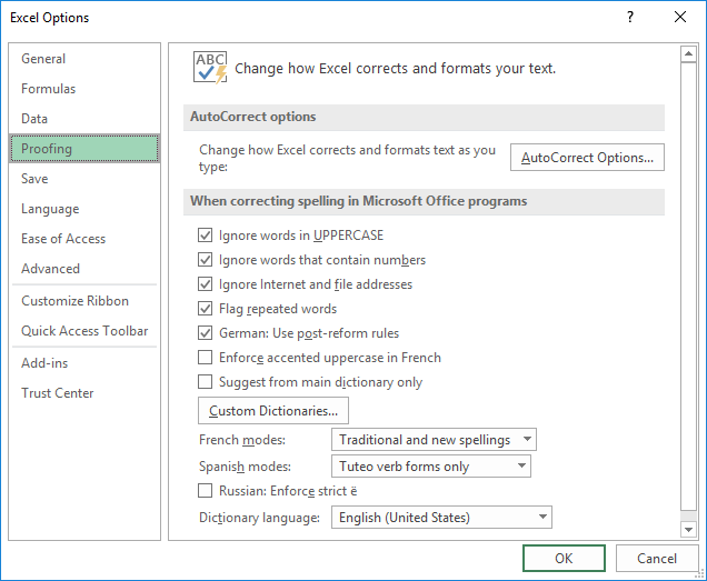
Excel spell check not working
If spell check does not work properly in your worksheet, try these simple troubleshooting tips:
Spelling button is greyed out
Most likely your worksheet is protected. Excel spell check does not work in protected sheets, so you will have to unprotect your worksheet first.
You are in edit mode
When in edit mode, only the cell you are currently editing is checked for spelling errors. To check the whole worksheet, exit the edit mode, and then run spell check.
Text in formulas is not checked
Cells containing formulas are not checked. To spell check text in a formula, get in the edit mode.
Find typos and misprints with Fuzzy Duplicate Finder
In addition to the built-in Excel spell check functionality, the users of our Ultimate Suite can quickly find and fix typos by using a special tool that resides on the Ablebits Tools tab under Find and Replace: 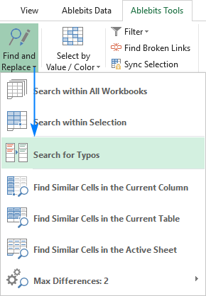
Clicking the Search for Typos button opens the Fuzzy Duplicate Finder pane on the left side of your Excel window. You are to select the range to check for typos and configure the settings for your search:
- Max number of different characters — limit the number of differences to look for.
- Min number of characters in a word/cell — exclude very short values from the search.
- The cells contain separate words delimited by — select this box if your cells may contain more than one word.
With the settings properly configured, click the Search for typos button. 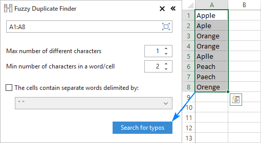
The add-in starts searching for values that differ in 1 or more characters, as specified by you. Once the search is finished, you are presented with a list of the found fuzzy matches grouped in nodes like shown in the screenshot below.
Now, you are to set the correct value for each node. For this, expand the group, and click the check symbol in the Action column next to the right value: 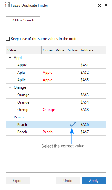
If the node doesn’t contain the right word, click in the Correct Value box next to the root item, type the word, and press Enter . 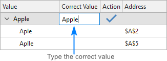
Upon assigning the correct values to all the nodes, click the Apply button, and all the typos in your worksheet will be fixed in one go: 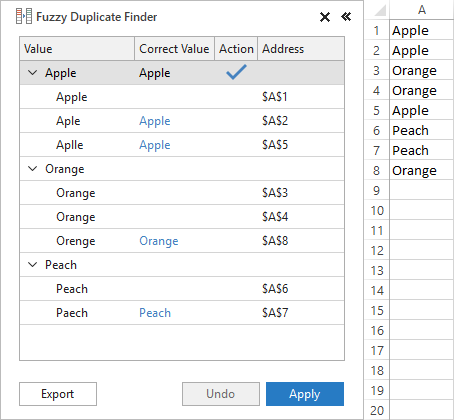
That’s how you perform spell check in Excel with Fuzzy Duplicate Finder. If you are curious to try this and 70+ more professional tools for Excel, you are welcome to download a trial version of our Ultimate Suite.
Источник
Когда работаешь много, то неизбежны ошибки. В конце концов не ошибается тот, кто ничего не делает. Исправить ошибки поможет проверка орфографии в Excel.
Скачайте файл тут. Я преднамеренно сделала несколько глупых ошибок, чтобы показать, как работает проверка орфографии в Excel. Откройте файл.
По окончании урока вы сможете:
- Настроить параметры операции «Проверка орфографии в Excel»
- Рассказать о командах диалогового окна «Орфография»
- Проверить орфографию на листе
- Скорректировать словарь
Шаг 1. Находим команду «Параметры» (Файл → Параметры):

Шаг 2. Отмечаем в диалоговом окне нужные режимы:

Я всегда отмечаю «Русский: требовать точного использования ё». Но в официальных документах «ё» не обязательно и это очень обедняет письменную речь.
| Это интересно! | 24 декабря 1942 года приказом народного комиссара просвещения РСФСР В.П. Потёмкина было введено обязательное употребление буквы «ё» везде: в школьных учебниках, переписках, газетах. И на картах, разумеется. Между прочим, этот приказ никто никогда не отменял А фамилия французского актёра будет Депардьё, а не Депардье. И правильно произносить фамилию русского поэта на самом деле нужно Фёт, а не Фет. |
2. Диалоговое окно «Орфография»
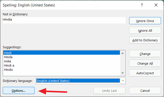
Шаг 1. Запускаем диалоговое окно «Орфография» (лента Рецензирование → группа команд Правописание → команда Орфография):

После выполнения команды может появится окно:

Окно появляется в том случае, если ваш курсор находится в любом месте листа. Отсюда следует очень интересный вывод:
| Понять и запомнить! | Можно назначить операцию «Проверка орфографии в Excel» только для выделенного диапазона |

Для выделенного диапазона A4:C9 проверка начинается с ячейки A4. Ячейка A3 с ошибочным словом «Касета для СD» выпадает из операции «Проверка орфографии в Excel»
Шаг 2. Изучаем диалоговое окно «Орфография»

- Пропустить (Ignore Once) – игнорировать ошибку в данном месте.
- Пропустить все (Ignore Аll) – не воспринимать данное слово как ошибку по всему листу.
- Добавить в словарь (Add to Dictionary) – добавить слово в словарь программы, чтобы в дальнейшем оно не воспринималось как ошибочное.
- Заменить (Change) – заменить ошибочное слово на то, которое выбрано в поле Варианты.
- Заменить все (Change Аll) – заменить ошибочное слово во всех местах по тексту на элемент списка, выбранный из поля Варианты.
- Автозамена (Autocorrect) – добавление ошибочного слова вместе с правильным словом из поля Варианты в функцию Автозамены для того, чтобы в дальнейшем такая ошибка автоматически исправлялась на правильный вариант.
- Это не команда, а поле Варианты, в котором вам предлагаются варианты замены ошибочного слова
3. Проверка орфографии в Excel
Шаг 1. Щелкаем по кнопке Заменить (Change) → слово «Наиминование» будет заменено на правильное и найдено следующее неизвестное слово «Касета».
Шаг 2. Щелкаем по кнопке Заменить (Change) → слово «Касета» будет заменено на правильное и найдено следующее неизвестное слово и так далее
Исправляем таким образом ошибки, пока не доберемся до слова «Безбарьерная». Чаще всего я работаю с техническими текстами, а технические термины в словарь не занесены. В результате весь документ подчеркнут красной волнистой чертой. Почему я вспомнила про Word?
4. Внесение слова в словарь
Как видите, проверка орфографии в Excel предлагает нам вариант «Безбарьерная
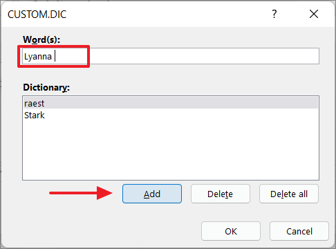
Шаг 1. Добавляем слово в словарь

А теперь посмотрим на наш словарь.
Шаг 2. Открываем диалоговое окно «Настраиваемые словари» (Файл → Параметры Word → Правописание → Настраиваемые словари):

Шаг 3. Отмечаем словарь «RoamingCustom.dic (по умолчанию)»:

Как видите, в моем словаре довольно приличное количество специальных терминов, которые офисные программы без моего вмешательства в словари отмечали, как ошибки. Но эти слова я добавлялf, работая в других офисных программах.

| Понять и запомнить! | Словарь проверки нашей грамотности единый для всех офисных программ! Что не может не радовать! |
В диалоговом окне «RoamingCustom.dic (по умолчанию)» вы можете добавлять слова, удалять одно слово или все слова разом. Не пренебрегайте работай со словарём, тем более, что это не обременительно.
Когда вы закончите проверять орфографию, то будет выведено сообщение о том, что проверка орфографии в Excel закончена:

Назначить проверку орфографии можно простым нажатием функциональной клавиши F7.
Теперь вы сможете:
- Настроить параметры операции «Проверка орфографии в Excel»
- Рассказать о командах диалогового окна «Орфография»
- Проверить орфографию на листе
- Скорректировать словарь
Most people know about Microsoft Word and Powerpoint’s spell-check and AutoCorrect features, but do you know MS Excel also facilitates the spell-checking functionality. It’s not as powerful and advanced as Word’s, but it does offer basic spell-checking functions. It allows you to check the spelling of words in the cells of worksheets and make sure your sheets are mistake-free.
Unlike Microsoft Word and PowerPoint, Excel doesn’t automatically check for grammar issues or check your spelling as you type (by underlining them in red). MS Excel will only notify you of spelling errors when you run the spellcheck functionality manually. Also, Excel doesn’t check grammar errors.
Most of the time, we ignore the spelling errors in Excel, because we often work with numbers and formulas. But sometimes, you need to check if you’ve made any spelling mistakes when creating some reports and datasets that may have texts such as column and row labels or in an entire worksheet. Let’s learn how to perform a spell check in a single cell, multiple cells, an entire worksheet, multiple worksheets at once, or the entire workbook.
How to Perform Spell Check in Excel
You can easily perform a spelling check within Microsoft Excel by following these steps:
There are two ways to run the spell-check feature in Excel: You can either access the tool from the Excel Ribbon or by using the keyboard shortcut.
First, open a spreadsheet with some spelling errors and select any cell. Go to the ‘Review’ tab, click on the ‘Spelling’ button at the left in the Proofing group of Excel Ribbon.
Alternatively, you can also press the keyboard shortcut F7 function key to open the Spelling dialogue box. If you select any single cell in the spreadsheet, Excel will automatically check for spelling errors in the entire current spreadsheet.
Either way, it will open up the Spelling dialog box. Excel will start checking spelling errors in your worksheet and it will provide suggestions for the correct spelling.
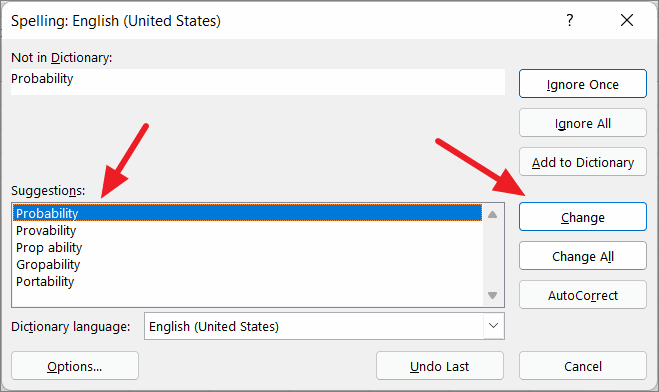
In the Spelling dialog, choose a suggestion from the ‘Suggestions:’ box and click the ‘Change’ button to correct the misspelling of the word. After that spelling has been corrected, it will move on to the next error. This box will only appear for the cells with misspelled words. Here, we will choose the first word ‘Probability’ from the suggestions list to replace the misspelled word ‘Propability’ and click on the ‘Change’ button.
Once all the spelling has been corrected, Excel will show you the ‘Spell check complete. You’re good to go’ message. Click ‘OK’ in the prompt box to continue.
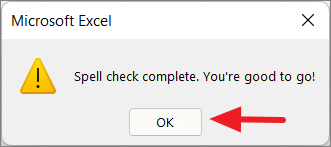
Excel will show you the Spelling dialog box only if there were any errors found in the sheet. If no error was found, Excel will show you the same above message.
If the spell check feature is not working (i.e the ‘Spelling’ button under the Review tab is greyed out.), it’s probably because your spreadsheet is protected. ‘Unprotect’ your worksheet before checking for spelling mistakes.
Different Options of Spelling Dialog Box
Before we learn how to perform spell check for cells, entire worksheets, multiple worksheets, or the entire workbook, we should understand the different options in the Spelling dialog box and how to customize them. You need to choose the appropriate options when correcting words.
The following are some of the functions you will see in the Spelling dialog box:
- Ignore Once – When spell check encounters a word that it identifies as an error, and the word is actually correct for your purposes, click on the ‘Ignore Once’ button to disregard the current spell check error suggestion. E.g. Names, Addresses, etc.
- Ignore All – Click this option, if you want to ignore all the instances of the current misspelled words and retain the original values. For example, if have the same name repeated multiple times, clicking this option will skip all those words without changing them and save you time.
- Add to Dictionary – If Excel regards the current word as an error, but it is a correct word and the one you use quite often, then you can add this misspelled word to the Microsoft Excel dictionary, as long as the word is used correctly. This will make the word as part of MS dictionary and will not be flagged as an error in the future in any workbook as well as in other Microsoft Products.
- Change – When a spell check error is detected, Excel will show you a list of suggestions. Select one of the suggested words and click this button to replace the currently selected misspelled word with the correct one.
- Change All – This option will replace all the occurrences of a misspelled word as well as the current one with the selected suggestion.
- AutoCorrect – Clicking this option will let Excel correct the misspelled word automatically with your selected suggestion. Also, it will add the word to the autocorrect list, which means if you type the same misspelled word in the future, Excel will automatically convert this to the selected suggestion.
- Dictionary language – You can change the Excel dictionary language using this drop-down.
- Options – This button will take you to ‘Excel Options’ where you can review or modify the default spell check settings accordingly.
- Undo Last – Click this button to reverse your last action.
Customizing the Settings of Excel Spell Check
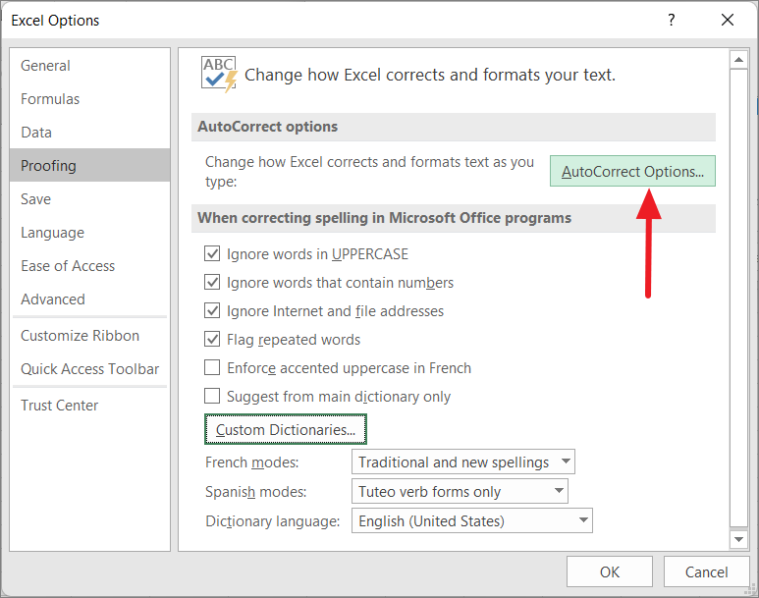
If you want to change the default settings of the Spell check in Excel, click ‘Options’ in the Spelling dialog box or go to the ‘File’ tab and click ‘Options.
In the Proofing tab of the Excel Options, you will find the default settings of the Spell check which you can customize as per your needs and requirements.
Excel ignores words that are in Upper Case (HEETHEN), text that contains numbers (Rage123), IP/file addresses, or internet codes and they will not be considered as a mistake. Also, it flags the repeated words as an error. E.g, if you type “Say hello to to my little friend”, it will flag, the additional ‘to’ as an error. You can enable or disable these options if you want.
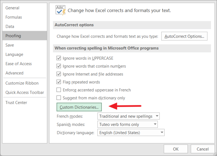
If you want to add or edit the Excel Dictionary, Click the ‘Custom Dictionaries’ option.
Then, to edit the list of words in the Custom Dictionaries, select the ‘CUSTOM.DIC’ under Dictionary List and click the ‘Edit Word List…’ button.
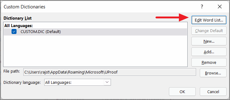
Enter the word you want to add to the dictionary in the ‘Word(s):’ field and click ‘Add’. If you want to remove an already added word from the list, select a word and click ‘Delete’ or ‘Delete all’ to remove all words. Then, click ‘OK’ twice to close both dialogs.
Also, any word added to the custom dictionaries will not be flagged as an error in any other Microsoft products. If you added a word to the custom dictionary in Excel, it will not be considered as an error in Word or Powerpoint and vice versa.
If you want to change the AutoCorrect settings, click the ‘AutoCorrect Options’ in Excel Options.
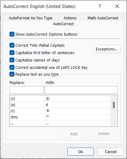
Here, you can customize the AutoCorrect settings.
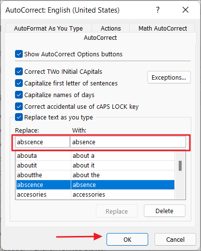
When typing, you may often misspell some words several times in your worksheet. You can fix these mistakes by adding those words to your AutoCorrect list. This way, Excel will autocorrect these words while you write.
To do this, enter the misspelled word in the ‘Replace’ section and select the correct word from the list below or enter it in the ‘With’ section. Then, click ‘OK’ to apply.
Spell Check a Single Cell/Text in Excel
Excel allows you to check a single cell value (Word) for spelling errors.
To check the spelling of any single cell in an Excel document, select the cell and double-click on it or press F2 to enter into edit mode. Make sure you are in the edit mode in the cell. If you’re in the edit mode, you will the text cursor in the cell and ‘Edit’ in the status bar at the bottom left corner of the Excel window (as shown below).
Then, click the ‘Spelling’ button in the Review tab or press F7.
If Excel finds any spelling errors it will display the suggestions box otherwise it will show a message with the message “The spelling check is complete”.
Select the correct word and click ‘Change’ to correct the spelling. Then, click ‘OK’ in the Spell check complete dialog box.

Spell Check Multiple Cells/Words in Single Worksheet
If you want to spell check multiple cells together, you can do that by selecting only those cells and using the Spelling dialog box. This method is useful when you want to skip the name or address column from checking errors because names and addresses are usually flagged as spelling errors.
First, select the cells or ranges or columns or rows you want to check for spelling. If you are selecting adjacent cells, then you simply use the mouse drag or Shift + arrow keys to make the selection.
If you want to select non-adjacent cells (cells that are not next to each other), you can press and hold the Ctrl key and click on the cells you want to get selected. If you have a large number of cells to select, press and release Shift + F8 and then click on as many cells as you want to select them. Then, press Shift + F8 again to turn off the selection mode.
Once you selected the cells, switch to the ‘Review’ tab and select ‘Spelling’ on the Ribbon or press F7.
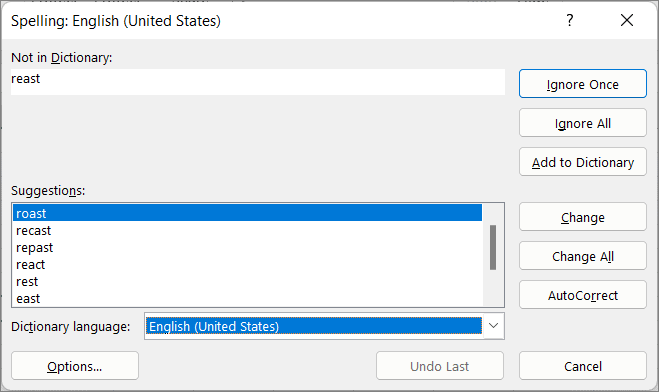
The Spelling dialog box will appear with some suggestions to replace the first misspelled word (if Excel found any) in the selected cells or ranges.
Then, select the correct suggestion, click on the ‘Change’ option or use ‘AutoCorrect’ to automatically select the correct spelling and move to the next misspelled word.
Or, you can also click ‘Ignore Once’ to dismiss the suggestion and move on to the next misspelled word.
Once, the first misspelled word has been corrected, it will show you suggestions for the next misspelled word in the same dialog box. Choose the appropriate options to fix the error. Similarly, you can correct all the misspelled words, one by one.
After all the misspelled words have been corrected, you will see the ‘success’ prompt.
Spell Check the Entire Worksheet
To spell-check an entire worksheet in Excel, select any cell in the worksheet you want to get checked or click the tab of the worksheet on which you want to run the spell check, and click on the ‘Spelling’ option (or press F7) under the ‘Review’ tab.
Excel will start checking for errors and give suggestions to correct them.
When you run the spell check, it checks for spelling from the currently selected cell and onward till the end of the worksheet. If you select cell A1, Excel will start checking all the cells in the first row (from left to right), then moves to the second row and check all the cells in the second row (from left to right) and then goes to the third row and so on.
For example, if you select A4, it will simply go through all cells of Row 4 (horizontally) and then rows below it. After checking for all the cells after A4, Excel will show you a prompt box, “Do you want to continue checking at the beginning of the sheet?”. Click ‘Yes’ to continuing the spell check from the beginning as shown below.
Spell-Check Multiple Sheets at Once
In Excel, you can check spellings for multiple worksheets together. Here’s how:
To check the spelling for the multiple worksheets, press and hold the Ctrl key and select the multiple sheet tabs that you want to check. Initiate spelling check by clicking the ‘Spelling’ button under the ‘Review’ tab or pressing the F7.
This will start the spell-checking process, and one by one, all the errors will pop up in the dialog box.
Choose appropriate options to fix all the errors and a dialog box will prompt to notify you with a confirmation message.
Spell Check All the Worksheets in a Workbook at Once
If you have many worksheets in your workbook, you can easily spell-check them all in one go.
To spell-check all the worksheets in a workbook, right-click on any worksheet’s tab and select ‘Select All Sheets’ from the context menu.
This will select all the worksheets in your workbook. Then, press F7 or click the ‘Spelling’ button under the Review ribbon tab. When all worksheets are selected, all the tabs will be displayed with a white background, as shown below.
Now Excel will spell-check all the worksheets in the workbook.
Spell Check Words in a Formula
If you try to check a text that is part of the formula, it won’t work and the spell-check runs back to the beginning of the worksheet. You can only check a text that is inside the shell of the formula in the edit mode.
If you want to check the spelling of the words in a formula, double-click on the cell with the formula or select the words inside the formula in the formula bar. Then, press F7 or click the ‘Spelling’ button under the Review ribbon tab to run the spell-check.
Highlight Spelling Mistakes using an Excel VBA Macro
You can even use the Excel Macro to find and highlight the misspelled words in the current worksheet. For this, you have to create a macro in the VBA editor. Here’s how you do this:
First, open the worksheet in which you want to highlight the misspelled words. Then, click the ‘Visual Basic’ button under the ‘Developer’ tab or press the shortcut key Alt + F11 to open the Excel VBA editor.
In the Microsoft VBA editor, click the ‘Insert’ menu and select the ‘Module’ option.
Then, copy and paste the following code in Module editor:
Sub ColorMispelledCells()
For Each cl In ActiveSheet.UsedRange
If Not Application.CheckSpelling(Word:=cl.Text) Then _
cl.Interior.ColorIndex = 8
Next cl
End Sub
After pasting the code click the ‘Run’ button in the toolbar or press the ‘F5’ key to run the macro.
Once you run the macro, check your worksheet. And all the cells with misspelled words would have been highlighted as shown below.
That’s everything you need to know about spell-checking in Excel.
Spell check in excel is a method of detecting spelling errors in text strings. Unlike MS Word and PowerPoint, MS Excel does not underline a misspelled word. As a result, a user may overlook spelling mistakes. Spell check in excel is beneficial when working with databases containing a mix of numbers and text.
For example, the cell references and text strings of a worksheet are listed as follows:
- Cell A1 consists of “Garden.”
- Cell A2 consists of “Kitchne.”
- Cell A3 consists of “Bulding.”
- Cell A4 consists of “Garage.”
On running a spell check, the “spelling” window opens. It shows the suggestions “kitchen” and “building.” Clicking “change” replaces the misspelled words (in cells A2 and A3) with the suggested options.
The purpose of spell check is to help the user deliver an error-free excel workbook. In addition, a spell check ensures that the text of the workbook is in accordance with the current proofing language.
In Excel, spell check is carried out either by pressing the shortcut F7 or by enabling AutoCorrect. Alternatively, one can click “spelling” from the “proofing” group of the Review tab. This is shown in the succeeding image.
The shortcut (F7) and the “spelling” button (under the Review tab) both open the “spelling” window. This window displays the suggested corrections.
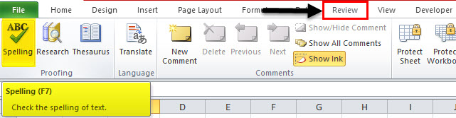
Table of contents
- How Spell Check in Excel Works?
- Example – Perform Spell Check in Excel
- The Spell Check Window in Excel
- The AutoCorrect in Excel
- The Features of the Spell Check in Excel
- Frequently Asked Questions
- Recommended Articles
How Spell Check in Excel Works?
Let us understand the working of the Excel spell check by assuming that the range A1:A10 consists of text strings. The user can select any of the following options as the starting point:
- Select cell A1–Excel checks the entire worksheet for spelling errors.
- Select cell A5 (or any other cell)–Excel checks for spelling errors beginning from cell A5 till the last data cell. Once it completes the spell check, a message asks whether to continue checking at the beginning of the sheet or not. The user is presented with the following options:
a. Yes–If this is clicked, Excel resumes checking from cell A1 and stops at cell A5.
b. No–If this is clicked, Excel stops checking at that point (last data cell of the worksheet).
You can download this Spell Check Excel Template here – Spell Check Excel Template
Example – Perform Spell Check in Excel
The following image shows the data of a worksheet. The spelling errors have been highlighted in bold. We want to run a spell check in excel using the shortcut key F7.
Assume the cell A1 as the starting point.

Step 1: Select cell A1 and press F7.
Step 2: The “spelling” dialog box opens, as shown in the succeeding image. The spelling “mostt” is “not in dictionary.” The suggested spelling is “most.”
Step 3: To accept the suggestion, click “change.” To ignore the suggestion, click “ignore once.”
Note: By pressing “ignore once,” the spelling “mostt” remains as is in the worksheet.

Step 4: Once a button is clicked in the preceding step (step 3), the next spelling mistake is displayed. The spelling “pwerful” is incorrect and “not in dictionary.” The suggested spelling is “powerful.”
Click “change” to replace the incorrect spelling with the correct one. Otherwise, click “ignore once” to retain the incorrect spelling as is.

Likewise, the spell check continues till the last data cell of the worksheet.
The Spell Check Window in Excel
The “spelling” dialog box is shown in the following image. Let us understand the functions of the options present on the left side of this window.

Not in dictionary: This shows the misspelled word which is not there in the Excel dictionary. Excel recognizes this word as a spelling mistake.

Suggestions: This displays one or more words which are similar in spelling to the misspelled word. These words are the corrections suggested by Excel.

Dictionary language: This is the selected language, which is adhered to, while checking for the misspelled words.
![]()
Let us understand the functions of the various options present on the right side of the “spelling” window. These options are shown with serial numbers in the following image.

In the succeeding pointers, every numbered bullet corresponds to the serial number of the preceding image. The options (shown in the preceding image) are explained as follows:
- Ignore once: Clicking this option ignores the current error. So, the misspelled word remains as is.
- Ignore all: With this option, all the instances of the misspelled word are ignored. So, all occurrences of the misspelled word remain as is.
- Add to the dictionary: This adds the current word to the dictionary. So, going forward, Excel will not identify this word as a spelling mistake. This option should be used if the spelling is correct, but is not present in the dictionary. For instance, an abbreviation or a person’s name can be added to the dictionary.
- Change: Clicking this option replaces the misspelled word with the suggested word. One can choose from the suggestions listed in the “spelling” window.
- Change all: This replaces all the instances of the misspelled word with the suggested word. Before clicking this option, one can select from the available suggestions.
- AutoCorrect: Clicking this option adds the misspelled word and the selected suggestion to the AutoCorrect list. So, going forward, if the same incorrect spelling is typed, Excel will auto-correct it. For example, the misspelled word is “nned” and the suggested word is “need.” With AutoCorrect, every time “nned” is typed, it will automatically be converted to “need.”
- Cancel: Clicking this option stops the spell check process and closes the “spelling” window. This can be clicked at any point of time.
The AutoCorrect in Excel
One can turn on or turn off the AutoCorrect feature of Excel. It is also possible to customize the same. The steps to customize the AutoCorrect feature are listed as follows:
- Click the File tab on the Excel ribbon.

- Click “options.”

- The “Excel options” window opens. Click “proofing.”

- Click “AutoCorrect options.”

- The “AutoCorrect” window appears, as shown in the succeeding image.
In the box under “replace,” type the words which need to be replaced. Type the replacements (corrections) in the box under “with.”
In other words, Excel is being told to replace the incorrect spellings (in the “replace” box) with the correct ones (in the “with” box).
Hence, the AutoCorrect feature can be customized as per the requirements of the user.
Note: The “AutoCorrect” window already lists the typical misspellings and their corrections that are used by default. One can change, add or delete entries from this list.


The Features of the Spell Check in Excel
The features of the Excel spell check are listed as follows:
- The spell check ignores the uppercase values. For example, if the word is “KITCHNE,” Excel does not recognize this as an error.
- The spell check does not correct grammatical errors, unlike MS Word.
- The default settings of the spell check can be changed by selecting “proofing” from “options” under the File tab.
- The excel spell check does not recognize a text string containing a number (in one cell) as an error. For example, if the word is “KITCHNE1,” it is not identified as an error.
- The spell check identifies the repeated words as errors. For example, in the string “this is the the kitchen,” the extra “the” is pointed as an error.
Frequently Asked Questions
1. What is spell check and where is it in Excel?
Spell check helps in checking the spellings of the Excel worksheet. With the spell check, the user can be assured that there are no spelling errors in the text strings.
Creating visually appealing graphs and charts in Excel are of no use if the text following them contains spelling mistakes. This is the reason why spell check is used in Excel. However, the Excel spell check cannot correct grammatical errors. Moreover, it does not underline the misspelled words.
The Excel spell check can be run by clicking “spelling” in the “proofing” group of the Review tab. The shortcut key for Excel spell check is F7.
2. How to run a spell check on the entire workbook of Excel?
The steps to perform a spell check on the entire workbook are listed as follows:
a. Right-click any sheet tab at the bottom-left side of Excel.
b. Choose “select all sheets” from the context menu. This selects all the sheets of the workbook.
c. Press F7 or click “spelling” from the “proofing” group of the Review tab.
Excel runs a spell check on all the worksheets of the current workbook. If there are any spelling errors (in any worksheet), the “spelling” window appears.
At the end of the process, Excel displays a message confirming that the spell check is complete.
3. How to change the dictionary language used in the spell check process of Excel?
The steps to change the dictionary language in Excel are listed as follows:
a. Click “spelling” in the “proofing” group of the Review tab.
b. The “spelling” window opens. Choose the desired language from the “dictionary language” drop-down.
c. Click “cancel” to close the “spelling” window.
d. Click “spelling” again from the Review tab. Excel begins the spell check with the newly selected language.
Hence, the dictionary language is changed.
Note: In case there are no spelling errors in the worksheet, the “spelling” window will not open. To change the dictionary language in such cases, misspell a word intentionally. In this way, the “spelling” window is made to appear.
Recommended Articles
This has been a guide to Spell Check in Excel. Here we discuss how to perform Spell Check in Excel along with step by step examples and shortcuts You may learn more about Excel from the following articles-
- Remove Space in ExcelWhile importing or copy-pasting the data from an external source, extra spaces are also copied in Excel. This makes the data disorganized and difficult to be used. The purpose of removing unwanted spaces from the excel data is to make it more presentable and readable for the user.
read more - Checkbox in ExcelA checkbox in excel is a square box used for presenting options (or choices) to the user to choose from.read more
- Excel Check MarkIn Excel, a check mark is used to indicate whether or not a task has been completed. There are three simple ways to enter a checkmark in Excel: 1) copy and paste a tick mark into the spreadsheet, 2) insert a symbol from the insert tab, 3) change the font to windings 2 and press the keyboard shortcut SHIFT+P.read more
- Checklist in ExcelIn Excel, a checklist is a checkbox that represents whether or not a given task has been completed. Normally, the value returned by the checklist is either true or false, but we may improvise the results. For example, when the checklist is ticked, the result is true; when it is blank, the result is false. The insert option on the developer’s tab allows you to insert a checklist.read more
- Forecast in ExcelThe FORECAST function in Excel is used to calculate or predict the future value based on existing values and the statistical value of the forecast. If we know the past data, we may use the function to forecast the future value.read more
A while back Vernon asked me how he could search one cell and compare it to a list of words. If any of the words in the list existed then return the matching word.
Ugh, I’ve written that 3 times and I’m not sure it’s any clearer…let’s look at an example.
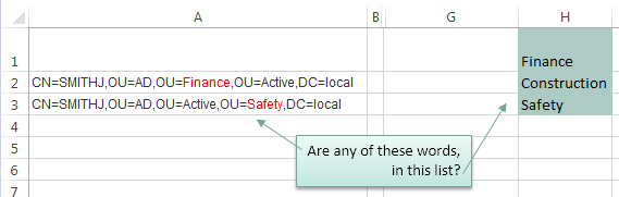
I’ve highlighted the matching words in column A red.
What we want Excel to do is to check the text string in column A to see if any of the words in our list in H1:H3 are present, if they are then return the matching word. Note: I’ve given cells H1:H3 the named range ‘list’.
There are a few ways we can tackle this so let’s take a look at our options.
Warning: this is quite an advanced topic which requires an array formula to solve it.
Update: It’s easier and more robust to use Power Query to search for text strings, including case and non-case sensitive searches.
Non-Case Sensitive Matching
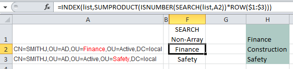
If you aren’t worried about case sensitive matches then you can use the SEARCH function with INDEX, SUMPRODUCT and ISNUMBER like this:
=INDEX(list,SUMPRODUCT(ISNUMBER(SEARCH(list,A2))*ROW($1:$3)))
In English our formula reads:
SEARCH cell A2 to see if it contains any words listed in cells H1:H3 (i.e. the named range ‘list’) and return the number of the character in cell A2 where the word starts. Our formula becomes:
=INDEX(list,SUMPRODUCT(ISNUMBER({20;#VALUE!;#VALUE!})*ROW($1:$3)))
i.e. in cell A2 the ‘F’ in the word ‘Finance’ starts in position 20.
Now using ISNUMBER test to see if the SEARCH formula returns any numbers (if it does it means there is a match). ISNUMBER will return TRUE if there is a number and FALSE if not (this gives us a list of Boolean TRUE or FALSE values). Our formula becomes:
=INDEX(list,SUMPRODUCT({TRUE;FALSE;FALSE}*ROW($1:$3)))
Use the ROW function to return an array of numbers {1;2;3} (see notes below on why I’ve used ROW in this formula). Our formula becomes:
=INDEX(list,SUMPRODUCT({TRUE;FALSE;FALSE}*{1;2;3}))
When you multiply Boolean TRUE/FALSE values they become their numeric equivalents i.e. TRUE = 1 and FALSE = 0. So our formula evaluates this ({TRUE;FALSE;FALSE}*{1;2;3}) like so: {1*1, 0*2, 0*3} and our formula becomes:
=INDEX(list,SUMPRODUCT({1;0;0}))
SUMPRODUCT simply sums the values {1+0+0} which gives us 1. Note: by using SUMPRODUCT we are avoiding the need for an array formula that requires CTRL+SHIFT+ENTER. Our formula becomes:
=INDEX(list,1)
Index can now go ahead and return the 1st value in the range of cells H1:H3 which is ‘Finance’.
Note: the above formula will not work if a match isn’t found. If you want to return an error if a match isn’t found then you can use this variation:
=INDEX(list,IF(SUMPRODUCT(--ISNUMBER(SEARCH(list,A2)))<>0,SUMPRODUCT(ISNUMBER(SEARCH(list,A2))*ROW($1:$3)),NA()))
Not as elegant, is it? In which case you might prefer one of the array formulas below.
Notes about the ROW Function:
The ROW function simply returns the row number of a reference. e.g. ROW(A2) would return 2. When used in an array formula it will return an array of numbers. e.g. ROW(A2:A4) will return {2;3;4}. We can also give just the row reference(s) to the ROW function like so ROW(2:4).
In this formula we have used ROW to simply return an array of values {1;2;3} that represent the items in our ‘list’ i.e. Finance is 1, Construction is 2 and Safety is 3. Alternatively we could have typed {1;2;3} direct in our formula, or even referenced the named range like this ROW(list).
So you see using the ROW function is just a quick and clever way to generate an array of numbers.
What you must bear in mind when using the ROW function for this purpose is that we need a list of numbers from 1 to 3 because there are 3 words in our list and we’re trying to find the position of the matching word.
In this example the formula; ROW(list) will also work because our list happens to start on row 1 but if we were to start ‘list’ on row 2 we would come unstuck because ROW(list) would return {2;3;4} i.e. ‘list’ would actually reference cells H2:H4.
So, don’t get confused into thinking the ROW part of the formula is simply referencing the list or range of cells where the list is, the important point is that the ROW formula returns an array of numbers and we’re using those numbers to represent the number of rows in the ‘list’ which must always start with 1.
Functions Used
INDEX
SEARCH or FIND
ISNUMBER
SUMPRODUCT
ROW — Explained above.
Case Sensitive Matching
[updated Dec 5, 2013]
If your search is case sensitive then you not only need to replace SEARCH with FIND, but you also need to introduce an IF formula like so:
=INDEX(list,IF(SUMPRODUCT(ISNUMBER(FIND(list,A2))*ROW($1:$3))<>0,SUMPRODUCT(ISNUMBER(FIND(list,A2))*ROW($1:$3)),NA()))
Unfortunately it’s not as simple or elegant as the first non-case sensitive search. Instead the array formulas below are nicer
Array Formula Options
Below are some array formula options to achieve the same result. They use LARGE instead of SUMPRODUCT, and as a result you need to enter these by pressing CTRL+SHIFT+ENTER.
Non-case Sensitive:
[updated Dec 5, 2013]
=INDEX(list,LARGE(IF(ISNUMBER(SEARCH(list,A2)),ROW($1:$3)),1)) Press CTRL+SHIFT+ENTER
Case sensitive:
[updated Dec 5, 2013]
=INDEX(list,LARGE(IF(ISNUMBER(FIND(list,A2)),ROW($1:$3)),1)) Press CTRL+SHIFT+ENTER
Download
Enter your email address below to download the sample workbook.
By submitting your email address you agree that we can email you our Excel newsletter.
Thanks
Special thanks to Roberto for suggesting the ‘updated’ formulas above.
This is an old question but a solution for those using Excel 2016 or newer is you can remove the need for nested if structures by using the new IFS( condition1, return1 [,condition2, return2] ...) conditional.
I have formatted it to make it visually clearer on how to use it for the case of this question:
=IFS(
ISERROR(SEARCH("String1",A1))=FALSE,"Something1",
ISERROR(SEARCH("String2",A1))=FALSE,"Something2",
ISERROR(SEARCH("String3",A1))=FALSE,"Something3"
)
Since SEARCH returns an error if a string is not found I wrapped it with an ISERROR(...)=FALSE to check for truth and then return the value wanted. It would be great if SEARCH returned 0 instead of an error for readability, but thats just how it works unfortunately.
Another note of importance is that IFS will return the match that it finds first and thus ordering is important. For example if my strings were Surf, Surfing, Surfs as String1,String2,String3 above and my cells string was Surfing it would match on the first term instead of the second because of the substring being Surf. Thus common denominators need to be last in the list. My IFS would need to be ordered Surfing, Surfs, Surf to work correctly (swapping Surfing and Surfs would also work in this simple example), but Surf would need to be last.