
This is an old question but a solution for those using Excel 2016 or newer is you can remove the need for nested if structures by using the new IFS( condition1, return1 [,condition2, return2] ...) conditional.
I have formatted it to make it visually clearer on how to use it for the case of this question:
=IFS(
ISERROR(SEARCH("String1",A1))=FALSE,"Something1",
ISERROR(SEARCH("String2",A1))=FALSE,"Something2",
ISERROR(SEARCH("String3",A1))=FALSE,"Something3"
)
Since SEARCH returns an error if a string is not found I wrapped it with an ISERROR(...)=FALSE to check for truth and then return the value wanted. It would be great if SEARCH returned 0 instead of an error for readability, but thats just how it works unfortunately.
Another note of importance is that IFS will return the match that it finds first and thus ordering is important. For example if my strings were Surf, Surfing, Surfs as String1,String2,String3 above and my cells string was Surfing it would match on the first term instead of the second because of the substring being Surf. Thus common denominators need to be last in the list. My IFS would need to be ordered Surfing, Surfs, Surf to work correctly (swapping Surfing and Surfs would also work in this simple example), but Surf would need to be last.
In this example, the goal is to test a value in a cell to see if it contains a specific substring. Excel contains two functions designed to check the occurrence of one text string inside another: the SEARCH function and the FIND function. Both functions return the position of the substring if found as a number, and a #VALUE! error if the substring is not found. The difference is that the SEARCH function supports wildcards but is not case-sensitive, while the FIND function is case-sensitive but does not support wildcards. The general approach with either function is to use the ISNUMBER function to check for a numeric result (a match) and return TRUE or FALSE.
SEARCH function (not case-sensitive)
The SEARCH function is designed to look inside a text string for a specific substring. If SEARCH finds the substring, it returns a position of the substring in the text as a number. If the substring is not found, SEARCH returns a #VALUE error. For example:
=SEARCH("p","apple") // returns 2
=SEARCH("z","apple") // returns #VALUE!
To force a TRUE or FALSE result, we use the ISNUMBER function. ISNUMBER returns TRUE for numeric values and FALSE for anything else. So, if SEARCH finds the substring, it returns the position as a number, and ISNUMBER returns TRUE:
=ISNUMBER(SEARCH("p","apple")) // returns TRUE
=ISNUMBER(SEARCH("z","apple")) // returns FALSE
If SEARCH doesn’t find the substring, it returns an error, which causes the ISNUMBER to return FALSE.
Wildcards
Although SEARCH is not case-sensitive, it does support wildcards (*?~). For example, the question mark (?) wildcard matches any one character. The formula below looks for a 3-character substring beginning with «x» and ending in «y»:
=ISNUMBER(SEARCH("x?z","xyz")) // TRUE
=ISNUMBER(SEARCH("x?z","xbz")) // TRUE
=ISNUMBER(SEARCH("x?z","xyy")) // FALSE
The asterisk (*) wildcard matches zero or more characters. This wildcard is not as useful in the SEARCH function because SEARCH already looks for a substring. For example, it might seem like the following formula will test for a value that ends with «z»:
=ISNUMBER(SEARCH("*z",text))However, because SEARCH automatically looks for a substring, the following formulas all return 1 as a result, even though the text in the first formula is the only text that ends with «z»:
=SEARCH("*z","XYZ") // returns 1
=SEARCH("*z","XYZXY") // returns 1
=SEARCH("*z","XYZXY123") // returns 1
=SEARCH("x*z","XYZXY123") // returns 1
This means the asterisk (*) is not a reliable way to test for «ends with». However, you an use the the asterisk (*) wildcard like this:
=SEARCH("x*2*b","AAAXYZ123ABCZZZ") // returns 4
=SEARCH("x*2*b","NXYZ12563JKLB") // returns 2
Here we are looking for «x», «2», and «b» in that order, with any number of characters in between. Finally, you can use the tilde (~) as an escape character to indicate that the next character is a literal like this:
=SEARCH("~*","apple*") // returns 6
=SEARCH("~?","apple?") // returns 6
=SEARCH("~~","apple~") // returns 6
The above formulas use SEARCH to find a literal asterisk (*), question mark (?) , and tilde (~) in that order.
FIND function (case-sensitive)
Like the SEARCH function, the FIND function returns the position of a substring in text as a number, and an error if the substring is not found. However, unlike the SEARCH function, the FIND function respects case:
=FIND("A","Apple") // returns 1
=FIND("A","apple") // returns #VALUE!
To make a case-sensitive version of the formula, just replace the SEARCH function with the FIND function in the formula above:
=ISNUMBER(FIND(substring,A1))
The result is a case-sensitive search:
=ISNUMBER(FIND("A","Apple")) // returns TRUE
=ISNUMBER(FIND("A","apple")) // returns FALSE
If cell contains
To return a custom result when a cell contains specific text, add the IF function like this:
=IF(ISNUMBER(SEARCH(substring,A1)), "Yes", "No")
Instead of returning TRUE or FALSE, the formula above will return «Yes» if substring is found and «No» if not.
With hardcoded search string
To test for a hardcoded substring, enclose the text in double quotes («»). For example, to check A1 for the text «apple» use:
=ISNUMBER(SEARCH("apple",A1))
More than one search string
To test a cell for more than one thing (i.e. for one of many substrings), see this example formula.
Excel for Microsoft 365 Excel 2021 Excel 2019 Excel 2016 Excel 2013 Excel 2010 Excel 2007 More…Less
Let’s say you want to ensure that a column contains text, not numbers. Or, perhapsyou want to find all orders that correspond to a specific salesperson. If you have no concern for upper- or lowercase text, there are several ways to check if a cell contains text.
You can also use a filter to find text. For more information, see Filter data.
Find cells that contain text
Follow these steps to locate cells containing specific text:
-
Select the range of cells that you want to search.
To search the entire worksheet, click any cell.
-
On the Home tab, in the Editing group, click Find & Select, and then click Find.

-
In the Find what box, enter the text—or numbers—that you need to find. Or, choose a recent search from the Find what drop-down box.
Note: You can use wildcard characters in your search criteria.
-
To specify a format for your search, click Format and make your selections in the Find Format popup window.
-
Click Options to further define your search. For example, you can search for all of the cells that contain the same kind of data, such as formulas.
In the Within box, you can select Sheet or Workbook to search a worksheet or an entire workbook.
-
Click Find All or Find Next.
Find All lists every occurrence of the item that you need to find, and allows you to make a cell active by selecting a specific occurrence. You can sort the results of a Find All search by clicking a header.
Note: To cancel a search in progress, press ESC.
Check if a cell has any text in it
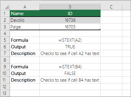
To do this task, use the ISTEXT function.
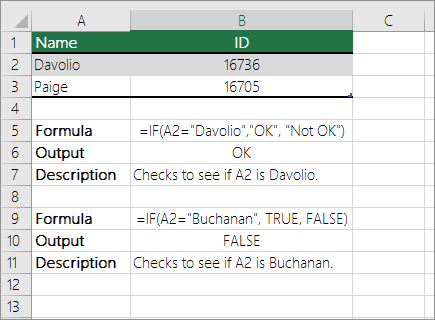
Check if a cell matches specific text
Use the IF function to return results for the condition that you specify.
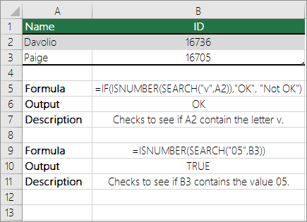
Check if part of a cell matches specific text
To do this task, use the IF, SEARCH, and ISNUMBER functions.
Note: The SEARCH function is case-insensitive.
Need more help?
To check if a cell contains specific text, use ISNUMBER and SEARCH in Excel. There’s no CONTAINS function in Excel.
1. To find the position of a substring in a text string, use the SEARCH function.

Explanation: «duck» found at position 10, «donkey» found at position 1, cell A4 does not contain the word «horse» and «goat» found at position 12.
2. Add the ISNUMBER function. The ISNUMBER function returns TRUE if a cell contains a number, and FALSE if not.

Explanation: cell A2 contains the word «duck», cell A3 contains the word «donkey», cell A4 does not contain the word «horse» and cell A5 contains the word «goat».
3. You can also check if a cell contains specific text, without displaying the substring. Make sure to enclose the substring in double quotation marks.

4. To perform a case-sensitive search, replace the SEARCH function with the FIND function.

Explanation: the formula in cell C3 returns FALSE now. Cell A3 does not contain the word «donkey» but contains the word «Donkey».
5. Add the IF function. The formula below (case-insensitive) returns «Found» if a cell contains specific text, and «Not Found» if not.

6. You can also use IF and COUNTIF in Excel to check if a cell contains specific text. However, the COUNTIF function is always case-insensitive.

Explanation: the formula in cell C2 reduces to =IF(COUNTIF(A2,»*duck*»),»Found»,»Not Found»). An asterisk (*) matches a series of zero or more characters. Visit our page about the COUNTIF function to learn all you need to know about this powerful function.
Generic formula to check a list of texts in a String (use CTRL + SHIFT + ENTER)

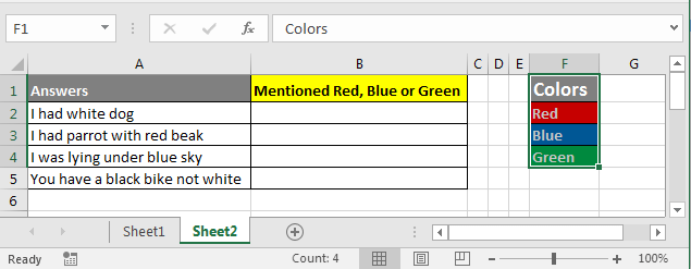
Scenario:
You have a survey data in which people have answered some questions. The data entry operator entered all data as it is. See the image below.

Now you have to know who mentioned any of these 3 colors Red, Blue and Green.
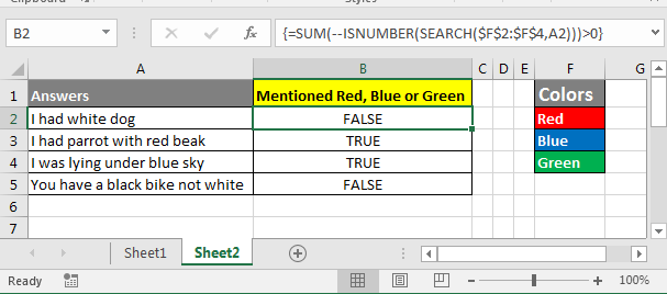
Write this formula in adjacent cell and hit CTRL+SHIFT+ENTER on the keyboard.
Drag it down and you have your answers. Now how many of your audience has mentioned these three colors in there statements.
How it Works
- CTRL + SHIFT + ENTER
- SEARCH($F$2:$F$4,A2) : The SEARCH looks for each value in the range $F$2:$F$4 and returns an array of found locations or #VALUE! Errors. For cell A2 it returns {#VALUE!;#VALUE!;#VALUE!} for A3 it will return {#VALUE!;#VALUE!;1}.
- ISNUMBER(SEARCH($F$2:$F$4,A2)) : ISNUMBER checks if supplied value in array is a number or not, if its number it returns TRUE else FALSE. For cell A2 it returns {FALSE;FALSE;FALSE} for A3 it will return {FALSE;FALSE;TRUE}.
- ——ISNUMBER(SEARCH($F$2:$F$4,A2)) : The double unary operator “——” converts TRUE into 1 and FALSE to 0. For cell A2 it returns {0;0;0} and for A3 it will return {0;0;1}.
- SUM(——ISNUMBER(SEARCH(list of strings, string))) : SUM function sum the array. For cell A2 it returns 0 and for A3 it will return 1.
- SUM(—ISNUMBER(SEARCH(list of strings, string)))>0 : Finally we check if sum of array is greater than 0 or not. If greater than 0, it means there is at least one mention of given colors and returns TRUE else FALSE.
- Using this function you can check multiple texts or say substrings in a string in one stance. To learn more about amazing function of EXCEL 2016, 2013 and 2010 or older go to our home page. We have a large list of useful excel articles.
Related Articles:
Sum if cells contain specific text
Sum if cell contains text in other cell in Excel
Count Cells that contain specific text
Split Numbers and Text from String in Excel
Highlight cells that contain specific text
Popular Articles:
50 Excel Shortcuts to Increase Your Productivity
How to use the VLOOKUP Function in Excel
How to use the COUNTIF function in Excel
How to use the SUMIF Function in Excel

Update: Based on questions I’ve received, I added the Misc Notes section to the end of this post.
Continuing with our #FunctionFriday series, today we’re going to explore how to use the IF, SEARCH, and ISNUMBER functions together to find text (aka a string) inside other text for classification purpose. What Excel really needs is a CONTAINS function, so we don’t have to do these mental acrobats. But, for now, this is what we have to work with.
To illustrate it, I’ll use an example from a chart I include in client dashboards** where they use the AddThis or ShareThis WordPress plugin. The data from these plugins populates to your Google Analytics account. BUT the data is such a red-hot mess, you have to do some cleanup to get it all into nice, neat buckets.
If you’d like to include this report in your own reports, you can use this custom report I created. (If you get a 404 error, it’s because you’re not logged in to Google Analytics. You have to be logged in to apply the report to your Google Analytics profile, aka view.)
**If you want to become a beast at building dashboards using the Google Analytics API, my online course will take you there.
Download Excel Workbook
If you’d like to follow along, you can download the Excel workbook I used in this demo.
The Functions du Jour
IF Function
The IF function is the Swiss Army knife for marketers, especially when you’re building out dynamic dashboards. With the IF function you start with a test — e.g., if A3=B2, if A3>=100, if A3=”organic”, etc. — and then you specify what you want to return if the condition is true and what you want to return if the value is false. But the fun doesn’t stop there; you can actually embed IF functions inside of IF functions. And that’s what we’re going to do in this tutorial.
It follows the following syntax:
IF(logical_test, [value_if_true], [value_if_false])
SEARCH Function
The SEARCH function is a tricky little bugger. It returns the position of whatever character you search for. And if you enter a string of characters, it will return the position of the first character in the matching string. So if you searched for cheese in the string string cheese, it would return the value of 8.
The SEARCH function follows the following syntax:
SEARCH( substring, string, [start_position] )
substring: Pure, unbridled geek speak that means whatever text you’re searching for, e.g., cheese.
string: Typically the cell this text string is in, though you could enter text as long as you flank it with quotation marks. (I almost always use a cell reference.)
start_position: This is optional. I usually only use it when I’m searching for forward slashes in URLs and want to start searching after the http(s)://. You can check out an example in this post that describes how to extract domains from URLs.
Now, if you put a string inside a SEARCH function, it will look for that string exactly. But you can also throw the asterisk wildcard in there for a really good time, which tells Excel to flag any string that even contains the text you’re searching for. So going back to our string cheese example, if I searched for cheese, it would return FALSE; if I searched for *cheese*, it would return TRUE.
ISNUMBER Function
The ISNUMBER function simply tells you if the cell you’re referencing is a value (or number). It’s Boolean, meaning it returns either a value of TRUE or FALSE.
It follows the following syntax:
ISNUMBER(value)
Pro Tip
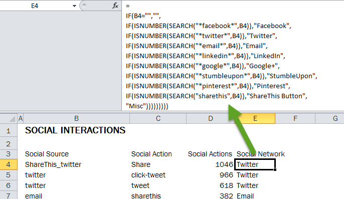
When dealing with a more complicated IF function, like you’ll see below, a good strategy is to break it into separate lines in the formula bar. To add a line break on a PC, use Alt-Enter; on a Mac, use Control-Option-Enter. I break my IF functions into different lines if I have more than three nested IFs. Here’s what it looks like for the formula we’ll use:
If you fat finger something in your formula, it’s really easy to see using this strategy because the IF functions won’t line up. When I’m finished, I just collapse the formula bar back to size by clicking-and-dragging the bottom of it.
Here’s what that same formula would look like if I didn’t use line breaks:

Putting It All Together
Okay, so here’s how we’re going to use them in concert. The Google Analytics custom report we’re using in this demo uses two dimensions: Social Source and Social Action and one metric, Social Actions. It’s a flat report, which, betedubs, is perfect for pivot tables. (Again, you should have data in this report if you use the ShareThis or AddThis plugin on WordPress.) But you could use this same strategy with any marketing data that you have to bucket based on snippets of text inside of strings.
If the formula in cell E4 could talk in plain English (wouldn’t that be nice?), here’s what it would say: “Hey, Excel, check out cell B4. If you see the string facebook anywhere in there, ISNUMBER will return a value of TRUE because you’ll return a number telling me the position of where the string I’m searching for. I don’t actually care about where that string is, only that it returns a number. If it does (IOW, it returns a value of TRUE), return the string Facebook; if it’s false, look for the next sting (i.e., twitter) and return Twitter … Rinse and repeat until you’ve cycled through all of the criteria. And if you don’t find facebook, twitter, email, linkedin, google, stumbleupon, pinterest, or sharethis, just call it Misc.” (Obviously, switch out sharethis for addthis if you’re using that plugin.)
Misc Notes
Difference Between SEARCH and FIND
Someone asked me about using the FIND function on Facebook instead of SEARCH. I rarely use the FIND function because it’s not as flexible as SEARCH. For one, it’s case sensitive. I can only remember one time using it because I needed to differentiate between cases. A much bigger liability is you can’t use it for partial matches because it doesn’t support Excel’s wildcard characters (* and ?).
Extracting Text Instead Of Categorizing It
So what if you didn’t want to match exact or partial text for the purpose of categorizing it like I have in this post with the help of the IF and ISNUMBER functions? What if, instead, you wanted to extract it instead? Then you would use the SEARCH function with the LEFT, RIGHT, and/or MID functions. I demonstrate how to do that in this tutorial on pulling domain names from a list of URLs. (I use this technique in conjunction with pivot tables in just about all competitive analysis I do because it allows me to group backlinks by domain.)
Image credit
~~~
If you would like to learn more about Excel, check out my Excel dashboard course. 24 instructional videos, totaling 6+ hours of instruction for $95.

Author: Oscar Cronquist Article last updated on October 19, 2021

This article demonstrates different formulas based on if a cell contains a given text.
Formula in cell C3:
=B3=$E$3
The formula shown in the image above in cell C3 returns TRUE or FALSE based on a comparison between cell B3 and cell E3. The equal sign is a logical operator and returns boolean value TRUE or FALSE, it is not case sensitive.
Table of Contents
- If cell contains partial text
- Explaining formula
- If cell contains partial text — hardcoded asterisks
- Alternative function — SEARCH function
- If cell contains text then return value
- If cell contains text then add text in another cell
- If cell contains text then sum
- If cell contains text add 1
- Highlight cell if cell contains text (Link)
- Get Excel file
1. If cell contains partial text

The easiest way to check if a cell partially contains a specific text string is, in my opinion, the IF and COUNTIF function combined. The COUNTIF function allows you to count how many times a text string exists in a cell range.
Formula in cell D3:
=IF(COUNTIF(B3, C3), TRUE, FALSE)
The asterisk characters let you perform a wildcard match meaning that it matches any sequence of characters. Adding a beginning and ending asterisk to a text string allows you to check if a cell value contains a specific text string.
Back to top
1.1 Explaining formula in cell D3
Step 1 — Check if cell contains text condition
You can’t use asterisks with the equal sign to check if a cell contains a given text, however, the COUNTIF function can do that.
The COUNTIF function calculates the number of cells that is equal to a condition.
COUNTIF(range, criteria)
COUNTIF(B3, C3)
becomes
COUNTIF(«Green, red and blue»,»*red*»)
and returns 1.
Step 2 — Evaluate IF function
The IF function returns one value if the logical test is TRUE and another value if the logical test is FALSE.
IF(logical_test, [value_if_true], [value_if_false])
IF(COUNTIF(B3, C3), TRUE, FALSE)
becomes
IF(1, TRUE, FALSE)
The logical_test argument requires boolean values or their numerical equivalents. FALSE = 0 (zero), TRUE any number except zero.
Back to top
1.2 If cell contains partial text — hardcoded asterisks

Formula in cell D4:
=IF(COUNTIF(B4, «*»&C4&»*»), TRUE, FALSE)
You don’t have to add asterisks manually to your cell, you can easily build a formula that adds the asterisks automatically, demonstrated in cell D4. The ampersand & character lets you append the asterisks to the text string you want to use.
Note, if a text string is found twice in the same cell the COUNTIF function only returns 1. It counts cells not text strings.
Back to top
1. Alternative function — SEARCH function
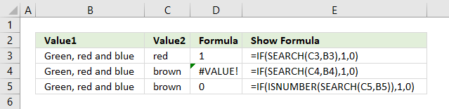
The SEARCH function returns the position of the character at which a specific text string is found. Luckily the IF function accepts any number as TRUE except 0 (zero), however, the SEARCH function returns an error #VALUE! if it can’t find the text string.
Formula in cell D5:
=IF(ISNUMBER(SEARCH(C5, B5)),1,0)
To avoid the error value I use the ISNUMBER function that returns TRUE if a number and FALSE if anything else, also formula errors.
Back to top
2. If cell contains text then return value

The formula in cell C3 checks if cell B3 contains the condition specified in cell E3. It returns the value if TRUE and a blank cell if FALSE.
Formula in cell C3:
=IF(COUNTIF(B3, «*»&$E$3&»*»), B3, «»)
Back to top
2.1 Explaining formula in cell C3
Step 1 — Concatenate strings
The asterisk is a wildcard character that matches 0 (zero) to any number of characters. The ampersand character concatenates strings in an Excel formula.
«*»&$E$3&»*»
becomes
«*»&»purple»&»*»
and returns «*purple*».
Step 2 — Check if cell contains string
The COUNTIF function calculates the number of cells that is equal to a condition.
COUNTIF(range, criteria)
COUNTIF(B3, «*»&$E$3&»*»)
becomes
COUNTIF(«Green, red and blue», «*purple*»)
and returns 0 (zero). Purple is not found in cell B3.
Step 3 — Return value if TRUE
The IF function returns one value if the logical test is TRUE and another value if the logical test is FALSE.
IF(logical_test, [value_if_true], [value_if_false])
IF(COUNTIF(B3, «*»&$E$3&»*»), B3, «»)
becomes
IF(0, B3, «»)
and returns «» in cell C3.
Back to top
3. If cell contains text then add text from another cell

The formula in cell C3 checks if cell B3 contains the condition specified in cell E3. It returns the value concatenated with a value on the same row from column if TRUE and a blank cell if FALSE.
Formula in cell C3:
=IF(COUNTIF(B3, «*»&$F$3&»*»), B3&C3, «»)
Back to top
3.1 Explaining formula in cell C4
Step 1 — Concatenate strings
The asterisk is a wildcard character that matches 0 (zero) to any number of characters. The ampersand character concatenates strings in an Excel formula.
«*»&$E$3&»*»
becomes
«*»&»purple»&»*»
and returns «*purple*».
Step 2 — Check if cell contains string
The COUNTIF function calculates the number of cells that is equal to a condition.
COUNTIF(range, criteria)
COUNTIF(B4, «*»&$E$3&»*»)
becomes
COUNTIF(«Black, purple, white», «*purple*»)
and returns 1. Purple is found in cell B4.
Step 3 — Return concatenated value if TRUE
The IF function returns one value if the logical test is TRUE and another value if the logical test is FALSE.
IF(logical_test, [value_if_true], [value_if_false])
IF(COUNTIF(B4, «*»&$E$3&»*»), B4&C4, «»)
becomes
IF(0, B4&C4, «»)
becomes
IF(0, «Black, purple, white»&»#11», «»)
and returns «Black, purple, white#11» in cell D4.
Back to top
4. If cell contains text then sum

The formula in cell F3 checks if cells in column B contain the condition specified in cell E3 and sums the corresponding values in column C.
Formula in cell C3:
=SUM(ISNUMBER(SEARCH(E3, B3:B6))*C3:C6)
Back to top
4.1 Explaining formula in cell C4
Step 1 — Search for string
The SEARCH function returns a number representing the position of character at which a specific text string is found reading left to right. It is not a case-sensitive search.
SEARCH(find_text,within_text, [start_num])
SEARCH(E3, B3:B6)
becomes
SEARCH(«North», {«North, South»; «South, East»; «West, North, South»; «South, West»})
and returns {1; #VALUE!; 7; #VALUE!}.
Step 2 — Check if value in array is an error
The ISNUMBER function checks if a value is a number, returns TRUE or FALSE.
ISNUMBER(SEARCH(E3, B3:B6))
becomes
ISNUMBER({1; #VALUE!; 7; #VALUE!})
and returns {TRUE; FALSE; TRUE; FALSE}.
Step 3 — Multiply corresponding numbers
The asterisk lets you multiply numbers in an Excel formula. We are multiplying boolean values in this example.
ISNUMBER(SEARCH(E3, B3:B6))*C3:C6
becomes
{TRUE; FALSE; TRUE; FALSE}*{10; 15; 6; 2}
TRUE equals 1 and FALSE equals 0 (zero).
{TRUE; FALSE; TRUE; FALSE}*{10; 15; 6; 2}
and returns {10; 0; 6; 0}.
Step 4 — Sum numbers
The SUM function adds numbers and returns a total.
SUM(ISNUMBER(SEARCH(E3, B3:B6))*C3:C6)
becomes
SUM({10; 0; 6; 0})
and returns 16 in cell F3.
Back to top
5. If cell contains text add 1

The formula in cell C3 counts cells containing the given text string in cell E3.
Formula in cell C3:
=IF(COUNTIF(B3,»*»&$E$3&»*»),1+MAX($C$2:C2),»»)
Back to top
5.1 Explaining formula in cell C3
Step 1 — Concatenate strings
The asterisk is a wildcard character that matches 0 (zero) to any number of characters. The ampersand character concatenates strings in an Excel formula.
«*»&$E$3&»*»
becomes
«*»&»North»&»*»
and returns «*North*».
Step 2 — Check if cell contains given string
The COUNTIF function calculates the number of cells that is equal to a condition.
COUNTIF(range, criteria)
COUNTIF(B3,»*»&$E$3&»*»)
becomes
COUNTIF(«North, South», «*North*»)
and returns 1.
Step 3 — Calculate count
The MAX function returns the largest number from a cell range or array.
Reference $C$2:C2 contains both absolute and relative cell references which makes it grow when the cell is copied to cells below.
1+MAX($C$2:C2)
becomes
1+0
and returns 1.
Step 4 — Show count if corresponding cell contains given string
The IF function returns one value if the logical test is TRUE and another value if the logical test is FALSE.
IF(logical_test, [value_if_true], [value_if_false])
IF(COUNTIF(B3,»*»&$E$3&»*»),1+MAX($C$2:C2),»»)
becomes
IF(C1,1+MAX($C$2:C2),»»)
becomes
IF(C1, 1, «»)
and returns 1.
Back to top
6. Get Excel *.xlsx file
Back to top