Check formulas in excel

Excel for Microsoft 365 Excel for Microsoft 365 for Mac Excel 2021 Excel 2021 for Mac Excel 2019 Excel 2019 for Mac Excel 2016 Excel 2016 for Mac Excel 2013 Excel 2010 Excel 2007 Excel for Mac 2011 Excel Starter 2010 More…Less

Formulas can sometimes result in error values in addition to returning unintended results. The following are some tools that you can use to find and investigate the causes of these errors and determine solutions.

Note: This topic contains techniques that can help you correct formula errors. It is not an exhaustive list of methods for correcting every possible formula error. For help on specific errors, you can search for questions like yours in the Excel Community Forum, or post one of your own.

Learn how to enter a simple formula

Formulas are equations that perform calculations on values in your worksheet. A formula starts with an equal sign (=). For example, the following formula adds 3 to 1.

=3+1

A formula can also contain any or all of the following: functions, references, operators, and constants.

Parts of a formula

Functions: included with Excel, functions are engineered formulas that carry out specific calculations. For example, the PI() function returns the value of pi: 3.142…
References: refer to individual cells or ranges of cells. A2 returns the value in cell A2.
Constants: numbers or text values entered directly into a formula, such as 2.
Operators: The ^ (caret) operator raises a number to a power, and the * (asterisk) operator multiplies. Use + and – add and subtract values, and / to divide.

Note: Some functions require what are referred to as arguments. Arguments are the values that certain functions use to perform their calculations. When required, arguments are placed between the function’s parentheses (). The PI function does not require any arguments, which is why it’s blank. Some functions require one or more arguments, and can leave room for additional arguments. You need to use a comma to separate arguments, or a semi-colon (;) depending on your location settings.

The SUM function for example, requires only one argument, but can accommodate 255 total arguments.

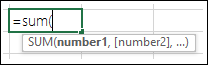
=SUM(A1:A10) is an example of a single argument.

=SUM(A1:A10, C1:C10) is an example of multiple arguments.

The following table summarizes some of the most common errors that a user can make when entering a formula, and explains how to correct them.

Make sure that you	More information
Start every function with the equal sign (=)	If you omit the equal sign, what you type may be displayed as text or as a date. For example, if you type SUM(A1:A10), Excel displays the text string SUM(A1:A10) and does not perform the calculation. If you type 11/2, Excel displays the date 2-Nov (assuming the cell format is General) instead of dividing 11 by 2.
Match all open and closing parentheses	Make sure that all parentheses are part of a matching pair (opening and closing). When you use a function in a formula, it is important for each parenthesis to be in its correct position for the function to work correctly. For example, the formula *=IF(B5<0),»Not valid»,B51.05) will not work because there are two closing parentheses and only one open parenthesis, when there should only be one each. The formula should look like this: =IF(B5<0,»Not valid»,B51.05)*.
Use a colon to indicate a range	When you refer to a range of cells, use a colon (:) to separate the reference to the first cell in the range and the reference to the last cell in the range. For example, =SUM(A1:A5), not =SUM(A1 A5), which would return a #NULL! Error.
Enter all required arguments	Some functions have required arguments. Also, make sure that you have not entered too many arguments.
Enter the correct type of arguments	Some functions, such as SUM, require numerical arguments. Other functions, such as REPLACE, require a text value for at least one of their arguments. If you use the wrong type of data as an argument, Excel may return unexpected results or display an error.
Nest no more than 64 functions	You can enter, or nest, no more than 64 levels of functions within a function.
Enclose other sheet names in single quotation marks	If a formula refers to values or cells on other worksheets or workbooks, and the name of the other workbook or worksheet contains spaces or non-alphabetical characters, you must enclose its name within single quotation marks ( ‘ ), like =’Quarterly Data’!D3, or =‘123’!A1.
Place an exclamation point (!) after a worksheet name when you refer to it in a formula	For example, to return the value from cell D3 in a worksheet named Quarterly Data in the same workbook, use this formula: =’Quarterly Data’!D3.
Include the path to external workbooks	Make sure that each external reference contains a workbook name and the path to the workbook. A reference to a workbook includes the name of the workbook and must be enclosed in brackets ([Workbookname.xlsx]). The reference must also contain the name of the worksheet in the workbook. If the workbook that you want to refer to is not open in Excel, you can still include a reference to it in a formula. You provide the full path to the file, such as in the following example: =ROWS(‘C:My Documents[Q2 Operations.xlsx]Sales’!A1:A8). This formula returns the number of rows in the range that includes cells A1 through A8 in the other workbook (8). Note: If the full path contains space characters, as does the preceding example, you must enclose the path in single quotation marks (at the beginning of the path and after the name of the worksheet, before the exclamation point).
Enter numbers without formatting	Do not format numbers when you enter them in formulas. For example, if the value that you want to enter is $1,000, enter 1000 in the formula. If you enter a comma as part of a number, Excel treats it as a separator character. If you want numbers displayed so that they show thousands or millions separators, or currency symbols, format the cells after you enter the numbers. For example, if you want to add 3100 to the value in cell A3, and you enter the formula =SUM(3,100,A3), Excel adds the numbers 3 and 100 and then adds that total to the value from A3, instead of adding 3100 to A3 which would be =SUM(3100,A3). Or, if you enter the formula =ABS(-2,134), Excel displays an error because the ABS function accepts only one argument: =ABS(-2134).

You can implement certain rules to check for errors in formulas. These rules do not guarantee that your worksheet is error free, but they can go a long way toward finding common mistakes. You can turn any of these rules on or off individually.

Errors can be marked and corrected in two ways: one error at a time (like a spell checker), or immediately when they occur on the worksheet as you enter data.

You can resolve an error by using the options that Excel displays, or you can ignore the error by clicking Ignore Error. If you ignore an error in a particular cell, the error in that cell does not appear in further error checks. However, you can reset all previously ignored errors so that they appear again.

For Excel on Windows, Click File > Options > Formulas, or
for Excel on Mac, click the Excel menu > Preferences > Error Checking.

In Excel 2007, click the Microsoft Office button > Excel Options > Formulas.
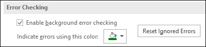
Under Error Checking, check Enable background error checking. Any error that is found, will be marked with a triangle in the top-left corner of the cell.
To change the color of the triangle that marks where an error occurs, in the Indicate errors using this color box, select the color that you want.
Under Excel checking rules, select or clear the check boxes of any of the following rules:
- Cells containing formulas that result in an error: A formula does not use the expected syntax, arguments, or data types. Error values include #DIV/0!, #N/A, #NAME?, #NULL!, #NUM!, #REF!, and #VALUE!. Each of these error values have different causes and are resolved in different ways.
  
  Note: If you enter an error value directly in a cell, it is stored as that error value but is not marked as an error. However, if a formula in another cell refers to that cell, the formula returns the error value from that cell.
- Inconsistent calculated column formula in tables: A calculated column can include individual formulas that are different from the master column formula, which creates an exception. Calculated column exceptions are created when you do any of the following:
  - Type data other than a formula in a calculated column cell.
  - Type a formula in a calculated column cell, and then use Ctrl +Z or click Undo on the Quick Access Toolbar.
  - Type a new formula in a calculated column that already contains one or more exceptions.
  - Copy data into the calculated column that does not match the calculated column formula. If the copied data contains a formula, this formula overwrites the data in the calculated column.
  - Move or delete a cell on another worksheet area that is referenced by one of the rows in a calculated column.
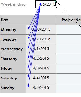
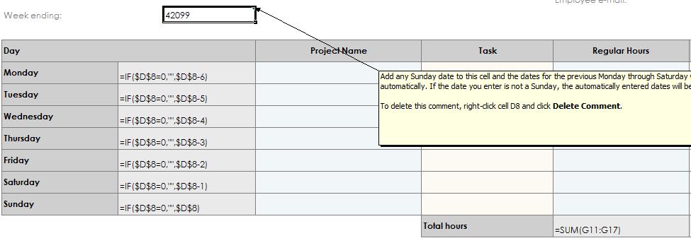
- Cells containing years represented as 2 digits: The cell contains a text date that can be misinterpreted as the wrong century when it is used in formulas. For example, the date in the formula =YEAR(«1/1/31») could be 1931 or 2031. Use this rule to check for ambiguous text dates.
- Numbers formatted as text or preceded by an apostrophe: The cell contains numbers stored as text. This typically occurs when data is imported from other sources. Numbers that are stored as text can cause unexpected sorting results, so it is best to convert them to numbers. ‘=SUM(A1:A10) is seen as text.
- Formulas inconsistent with other formulas in the region: The formula does not match the pattern of other formulas near it. In many cases, formulas that are adjacent to other formulas differ only in the references used. In the following example of four adjacent formulas, Excel displays an error next to the formula =SUM(A10:C10) in cell D4 because the adjacent formulas increment by one row, and that one increments by 8 rows — Excel expects the formula =SUM(A4:C4).
  
  If the references that are used in a formula are not consistent with those in the adjacent formulas, Excel displays an error.
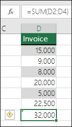
- Formulas which omit cells in a region: A formula may not automatically include references to data that you insert between the original range of data and the cell that contains the formula. This rule compares the reference in a formula against the actual range of cells that is adjacent to the cell that contains the formula. If the adjacent cells contain additional values and are not blank, Excel displays an error next to the formula.
  
  For example, Excel inserts an error next to the formula =SUM(D2:D4) when this rule is applied, because cells D5, D6, and D7 are adjacent to the cells that are referenced in the formula and the cell that contains the formula (D8), and those cells contain data that should have been referenced in the formula.
- Unlocked cells containing formulas: The formula is not locked for protection. By default, all cells on a worksheet are locked so they can’t be changed when the worksheet is protected. This can help avoid inadvertent mistakes like accidentally deleting or altering formulas. This error indicates that the cell has been set to be unlocked, but the sheet has not been protected. Check to make sure that you do not want the cell locked or not.
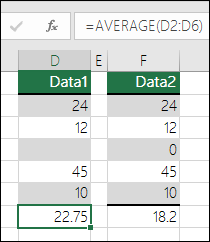
- Formulas referring to empty cells: The formula contains a reference to an empty cell. This can cause unintended results, as shown in the following example.
  
  Suppose you want to calculate the average of the numbers in the following column of cells. If the third cell is blank, it is not included in the calculation and the result is 22.75. If the third cell contains 0, the result is 18.2.
- Data entered in a table is invalid: There is a validation error in a table. Check the validation setting for the cell by going to the Data tab > Data Tools group > Data Validation.

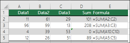
Select the worksheet you want to check for errors.
If the worksheet is manually calculated, press F9 to recalculate.

If the Error Checking dialog is not displayed, then click on the Formulas tab > Formula Auditing > Error Checking button.
If you have previously ignored any errors, you can check for those errors again by doing the following: click File > Options > Formulas. For Excel on Mac, click the Excel menu > Preferences > Error Checking.

In the Error Checking section, click Reset Ignored Errors > OK.

Note: Resetting ignored errors resets all errors in all sheets in the active workbook.

Tip: It might help if you move the Error Checking dialog box just below the formula bar.
Click one of the action buttons in the right side of the dialog box. The available actions differ for each type of error.
Click Next.

Note: If you click Ignore Error, the error is marked to be ignored for each consecutive check.

Next to the cell, click the Error Checking button that appears, and then click the option you want. The available commands differ for each type of error, and the first entry describes the error.

If you click Ignore Error, the error is marked to be ignored for each consecutive check.

If a formula cannot correctly evaluate a result, Excel displays an error value, such as #####, #DIV/0!, #N/A, #NAME?, #NULL!, #NUM!, #REF!, and #VALUE!. Each error type has different causes, and different solutions.

The following table contains links to articles that describe these errors in detail, and a brief description to get you started.

Topic	Description
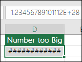
Correct a #### error	Excel displays this error when a column is not wide enough to display all the characters in a cell, or a cell contains negative date or time values. For example, a formula that subtracts a date in the future from a date in the past, such as =06/15/2008-07/01/2008, results in a negative date value. Tip: Try to auto-fit the cell by double-clicking between the column headers. If ### is displayed because Excel can’t display all of the characters this will correct it.
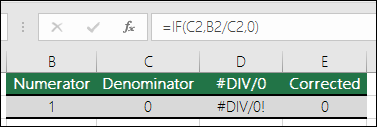
Correct a #DIV/0! error	Excel displays this error when a number is divided either by zero (0) or by a cell that contains no value. Tip: Add an error handler like in the following example, which is =IF(C2,B2/C2,0)
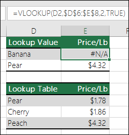
Correct a #N/A error	Excel displays this error when a value is not available to a function or formula. If you’re using a function like VLOOKUP, does what you’re trying to lookup have a match in the lookup range? Most often it doesn’t. Try using IFERROR to suppress the #N/A. In this case you could use: =IFERROR(VLOOKUP(D2,$D$6:$E$8,2,TRUE),0)
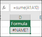
Correct a #NAME? error	This error is displayed when Excel does not recognize text in a formula. For example, a range name or the name of a function may be spelled incorrectly. Note: If you’re using a function, make sure the function name is spelled correctly. In this case SUM is spelled incorrectly. Remove the “e” and Excel will correct it.
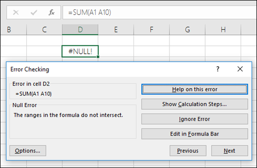
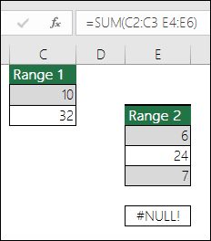
Correct a #NULL! error	Excel displays this error when you specify an intersection of two areas that do not intersect (cross). The intersection operator is a space character that separates references in a formula. Note: Make sure your ranges are correctly separated — the areas C2:C3 and E4:E6 do not intersect, so entering the formula =SUM(C2:C3 E4:E6) returns the #NULL! error. Putting a comma between the C and E ranges will correct it =SUM(C2:C3,E4:E6)
Correct a #NUM! error	Excel displays this error when a formula or function contains invalid numeric values. Are you using a function that iterates, such as IRR or RATE? If so, the #NUM! error is probably because the function can’t find a result. Refer to the help topic for resolution steps.
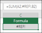
Correct a #REF! error	Excel displays this error when a cell reference is not valid. For example, you may have deleted cells that were referred to by other formulas, or you may have pasted cells that you moved on top of cells that were referred to by other formulas. Did you accidentally delete a row or column? We deleted column B in this formula, =SUM(A2,B2,C2), and look what happened. Either use Undo (Ctrl+Z) to undo the deletion, rebuild the formula, or use a continuous range reference like this: =SUM(A2:C2), which would have automatically updated when column B was deleted.
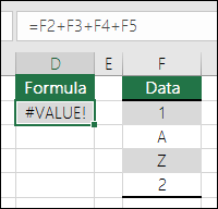
Correct a #VALUE! error	Excel can display this error if your formula includes cells that contain different data types. Are you using Math operators (+, -, *, /, ^) with different data types? If so, try using a function instead. In this case =SUM(F2:F5) would correct the problem.

When cells are not visible on a worksheet, you can watch those cells and their formulas in the Watch Window toolbar. The Watch Window makes it convenient to inspect, audit, or confirm formula calculations and results in large worksheets. By using the Watch Window, you don’t need to repeatedly scroll or go to different parts of your worksheet.

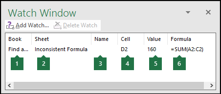
This toolbar can be moved or docked like any other toolbar. For example, you can dock it on the bottom of the window. The toolbar keeps track of the following cell properties: 1) Workbook, 2) Sheet, 3) Name (if the cell has a corresponding Named Range), 4) Cell address, 5) Value, and 6) Formula.

Note: You can have only one watch per cell.

Add cells to the Watch Window

Select the cells that you want to watch.

To select all cells on a worksheet with formulas, on the Home tab, in the Editing group, click Find & Select (or you can use Ctrl+G, or Control+G on the Mac)> Go To Special > Formulas.
On the Formulas tab, in the Formula Auditing group, click Watch Window.
Click Add Watch.
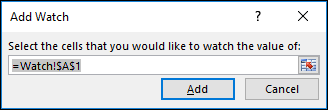
Confirm that you have selected all of the cells you want to watch and click Add.
To change the width of a Watch Window column, drag the boundary on the right side of the column heading.
To display the cell that an entry in Watch Window toolbar refers to, double-click the entry.

Note: Cells that have external references to other workbooks are displayed in the Watch Window toolbar only when the other workbooks are open.

Remove cells from the Watch Window

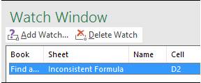
If the Watch Window toolbar is not displayed, on the Formulas tab, in the Formula Auditing group, click Watch Window.
Select the cells that you want to remove.

To select multiple cells, press CTRL and then click the cells.
Click Delete Watch.

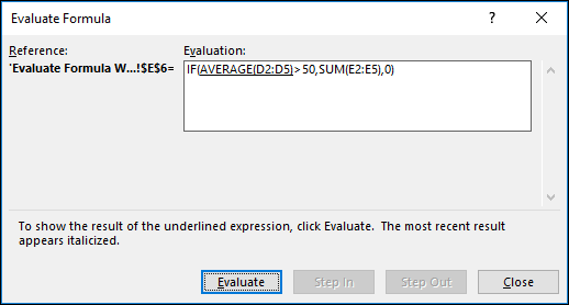
Sometimes, understanding how a nested formula calculates the final result is difficult because there are several intermediate calculations and logical tests. However, by using the Evaluate Formula dialog box, you can see the different parts of a nested formula evaluated in the order the formula is calculated. For example, the formula =IF(AVERAGE(D2:D5)>50,SUM(E2:E5),0)is easier to understand when you can see the following intermediate results:

In the Evaluate Formula dialog box	Description
=IF(AVERAGE(D2:D5)>50,SUM(E2:E5),0)	The nested formula is initially displayed. The AVERAGE function and the SUM function are nested within the IF function. The cell range D2:D5 contains the values 55, 35, 45, and 25, and so the result of the AVERAGE(D2:D5) function is 40.
=IF(40>50,SUM(E2:E5),0)	The cell range D2:D5 contains the values 55, 35, 45, and 25, and so the result of the AVERAGE(D2:D5) function is 40.
=IF(False,SUM(E2:E5),0)	Because 40 is not greater than 50, the expression in the first argument of the IF function (the logical_test argument) is False. The IF function returns the value of the third argument (the value_if_false argument). The SUM function is not evaluated because it is the second argument to the IF function (value_if_true argument), and it is returned only when the expression is True.

Select the cell that you want to evaluate. Only one cell can be evaluated at a time.
Select the Formulas tab > Formula Auditing > Evaluate Formula.
Click Evaluate to examine the value of the underlined reference. The result of the evaluation is shown in italics.

If the underlined part of the formula is a reference to another formula, click Step In to display the other formula in the Evaluation box. Click Step Out to go back to the previous cell and formula.

The Step In button is not available for a reference the second time the reference appears in the formula, or if the formula refers to a cell in a separate workbook.
Continue clicking Evaluate until each part of the formula has been evaluated.
To see the evaluation again, click Restart.
To end the evaluation, click Close.

Notes:

Some parts of formulas that use the IF and CHOOSE functions are not evaluated — in these cases, #N/A is displayed in the Evaluation box.
If a reference is blank, a zero value (0) is displayed in the Evaluation box.
The following functions are recalculated each time the worksheet changes, and can cause the Evaluate Formula dialog box to give results different from what appears in the cell: RAND, AREAS, INDEX, OFFSET, CELL, INDIRECT, ROWS, COLUMNS, NOW, TODAY, RANDBETWEEN.

Need more help?

You can always ask an expert in the Excel Tech Community or get support in the Answers community.

Transcript

One thing you’ll frequently do in Excel is check or debug formulas.

In this video, we’ll look at how to use the F9 key to quickly break a formula down into pieces that you can understand.

Here we have a simple list of names. In addition to names, we have a column for birthdate, a column for age, and a column for legal status.

We’ve covered this before, but whenever you inherit a new worksheet, make sure you understand first where the formulas are. You can do this quickly by using Go To Special > Formulas.

You can see that both Age and Status are calculated values.

Now let’s use the F9 key to see what the STATUS formula is doing.

In general, it’s easier to debug a formula in the formula bar. And you may want to expand the formula bar to give yourself more space to work.

Once you’re in Edit Mode, you can use the F9 key to check the calculated value of any part of the formula.

Although you can select parts of the formula manually, the Function Tooltip makes it much easier to select things precisely.

To display the tooltip, click directly on or inside any function. For example, when we click anywhere inside the IF function, we see its three arguments listed in the tooltip, and we can simply click to select each argument in the formula.

Once you have an argument selected, press the F9 key to evaluate. In this case, H5 evaluates to «Minor», H6 evaluates to «Adult», and the logical test evaluates to FALSE since Michael is only 12 years old.

Press the Escape key to exit the formula editor without making changes.

Pay attention to your selection before you press F9. If the cursor is outside the last set of parentheses, or if nothing is selected, you’ll see only the final result of the formula when you use F9. Again, press Escape to exit without making changes.

Now let’s look at the formula that calculates Age.

You can see that the formula uses two functions: YEARFRAC and INT.

Working from the inside out, we see the start date and end date both evaluate to date serial numbers. Next, the YEARFRAC function returns years as a fractional value. And finally, the INT function gives us just the integer value, which corresponds to a person’s age as of today.

Use the F9 key whenever you want to understand or debug a formula. It’s a great way to quickly understand how a formula works, and it will save you the trouble of breaking the formula down into separate formulas on the worksheet.

Источник

MS Excel is mainly used and famous for its function, formulas, and Macros. But what if we are getting some issues while writing the formula, or we cannot get the desired result in a cell as we have not formulated the function correctly? That is why MS Excel provides many built-in tools for auditing and troubleshooting formulas.

Formula Auditing Tools in Excel
- Examples of Auditing Tools in Excel
  - #1 – Trace Precedents
  - #2 – Remove Arrows
  - #3 – Trace Dependents
  - #4 – Show Formulas
  - #5 – Error Checking
- Things to Remember
- Recommended Articles

The tools which we can use for auditing and formula troubleshooting in ExcelTroubleshooting in Excel helps when we tend to get some errors or unexpected results associated with the formula we use in Excel. read more are:

Trace Precedents
Trace Dependents
Remove Arrows
Show Formulas
Error Checking
Evaluate FormulaThe Evaluate formula in Excel is used to analyze and understand any fundamental Excel formula such as SUM, COUNT, COUNTA, and AVERAGE. For this, you may use the F9 key to break down the formula and evaluate it step by step, or you may use the “Evaluate” tool.read more

Examples of Auditing Tools in Excel

We will learn about each of the above auditing tools using some examples in Excel.

You can download this Auditing Tools Excel Template here – Auditing Tools Excel Template

#1 – Trace Precedents

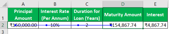
Suppose we have the following formula in the D2 cell for calculating interest for an FD account in a bank.

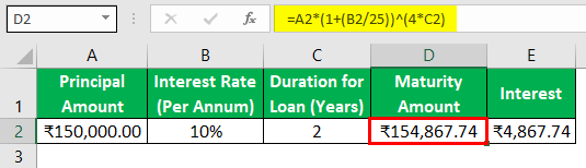
If we want to check the formula’s precedents, we can press F2 to get into edit mode after selecting the required cell so that precedents cells get bordered with various colors and written in the same color and cell reference.

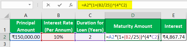
We can see that A2 is written with blue in the formula cell, and with the same color, the A2 cell is bordered.

In the same way,

B2 cell has a red color.

C2 cell has a purple color.

This way is good. But we have a more convenient way to check precedents for the formula cell.

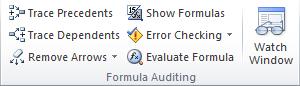
We can use the “Trace Precedents” command in the “Formula Auditing” group under the “Formulas” tab to trace precedents.

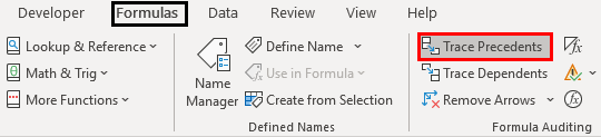
Select the formula cell and click on the “Trace Precedents” command. Then, you can see an arrow, as shown below.

We can see that precedent cells are highlighted with blue dots.

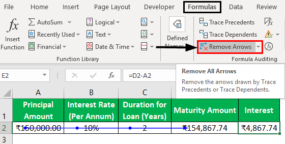
#2 – Remove Arrows

We can use the “Remove Arrows” command in the “Formula Auditing” group under the “Formulas” tab to remove these arrows.

#3 – Trace Dependents

This command traces the cell, dependent on the selected cell.

Let us use this command using an example.

Suppose we have four amounts that we can invest in. We want to know how much interest we can earn if we invest.

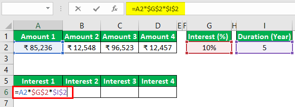
In the above image, we can see that we have applied a formula for calculating interest with Amount 1 and specified interest percentage and duration in the year.

We will copy the formula and paste it into the adjacent cells for Amount 2, Amount 3, and Amount 4. One can notice that we have used an absolute cell referenceAbsolute reference in excel is a type of cell reference in which the cells being referred to do not change, as they did in relative reference. By pressing f4, we can create a formula for absolute referencing.read more for G2 and I2 cells as we do not want to change these references while copying and pasting.

If we want to check which cells are dependent on the G2 cell, we will use the “Trace Dependents” command available in the “Formula Auditing” group under the “Formulas” tab.

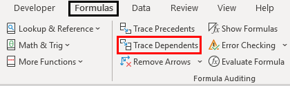
Select the G2 cell and click on the “Trace Dependents” command.

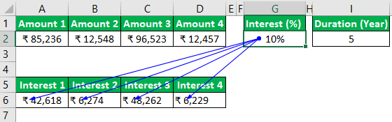
In the above image, we can see the arrow lines where arrows indicate which cells are dependent on the cells.

We will remove the arrow lines using the ‘Remove Arrows’ command.

#4 – Show Formulas

We can use this command to display formulas written in the excel sheet. The shortcut key for this command is ‘Ctrl+~.’

See the below image, where we can see the formulas in the cell.

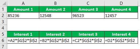
We can see that we can see the formula instead of the formula results. For amounts, the currency format is not visible.

Press ‘Ctrl+~’ again or click on the ‘Show Formulas’ command to deactivate this mode.

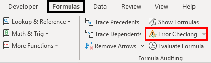
#5 – Error Checking

This command is used to check the specified formula or function error.

Let us take an example to understand this.

See the below image where we have an error in the function applied for the result.

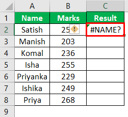
We will use the ‘Error CheckingWhen we insert a formula and forget to include some required input, we get an error in Excel. Some of the most common errors in Excel formulas are #NAME?, #DIV/0!, #REF!, #NULL!, #N/A, ######, #VALUE! and #NUM!.read more‘ command to solve this error.

The steps would be:

Select the cell where the formula or function is written, then click “Error Checking.”

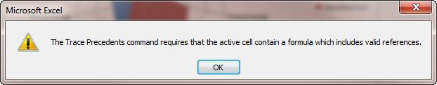
As we click on the command, we get the dialog box “Error Checking.”

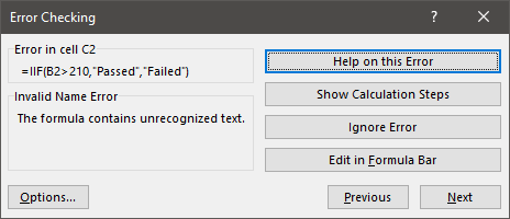
In the above dialog box, it can be seen that there is some invalid name error. Therefore, the formula contains the unrecognized text.

Suppose we use the function or construct the formula for the first time. In that case, we can click on the“Help on this Error” button, which will open the help page for the function in the browser, where we can see all the related information online, understand the cause, and find all the possible solutions.

We will find the following page as we click on this button now.

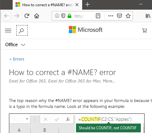
On this page, we get to know about the error that this error occurs when:

The formula refers to a name that has not been defined. For example, the function name or named range has not been described earlier.
The formula has a typo in the defined name. It means that there is some typing error.

If we have used the function earlier and know about the function, then we can click on the “Show Calculation Steps” button to check how the evaluation of the function results in an error.

If we click on this button, the following steps are displayed:

The next dialog box displays when we click the “Show Calculation Steps” button.

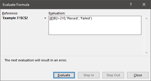
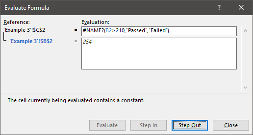
After clicking on the ‘Evaluate’ button, the underlined expression, i.e., ‘IIF,’ gets evaluated and gives the following information as displayed in the dialog box.

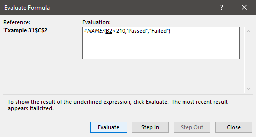
Does the above image show that the “IIF” expression is evaluated as an error; #NAME? The following expression or reference, i.e., B2, was underlined. If we click the “Step In” button, we can check the internal details and come out by pressing the “Step Out” button.

Now, we will click on the “Evaluate” button to check the result of the underlined expression. After clicking, we get the following result.

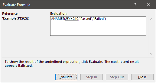
After clicking the “Evaluate” button, we get the result of the applied function.

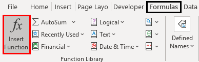
We got an error. As a result, as we analyzed the function step by step, we learned that there was some error in “IIF.” We can use the “Insert Function” command in the “Function Library” group under the “Formulas” tab.

As we typed the “IF,” we got a similar function in the list; we needed to choose the appropriate function.

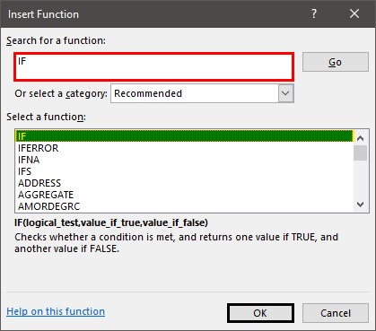
After selecting the “IF” function, we get the following dialog box with text boxes for argument, and we need to fill in all the details.

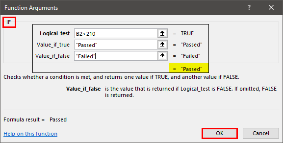
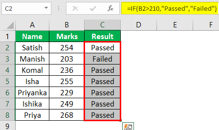
After clicking on “OK,“ we get the result in the cell. Next, we will copy down the function for all the students.

Things to Remember

The dates are also shown in the number format if we activate the ‘Show Formulas’ command.
While evaluating the formula, we can also use “F9” as a shortcut in ExcelAn Excel shortcut is a technique of performing a manual task in a quicker way.read more.

Tracing Formula Precedents and Dependents

Tracing precedents allows you to backtrack through all of the cells that are used to calculate a formula. This allows you to quickly find and identify what values a selected formula is dependent on. In the image below, we have selected cell D2. This cell contains a formula that calculates monthly payments:

Next, we clicked Formulas → Trace Precedents:

You will now see a blue arrow drawn across the current row, where all of the data used by the currently selected formula appears. Each blue dot on this arrow corresponds to a value that is used in the formula, while the arrowhead points to the end value. In this particular example, you can see that cells A2, B2, and C2 are all used by the formula in D2 to calculate the end value:

The Trace Dependents command works the opposite way of Trace Precedents: it highlights all the items that depend on the value in the current cell. This command will not work for values in the Monthly Payment column (D) because it has no dependents. However, the Loan Period (B) column does have dependents.

If we Click cell B4 and then click Formulas → Trace Dependents:

Another blue arrow will be drawn from the selected cell, pointing towards the dependent cell, which in this case is the formula in cell D4:

As you can see in the images, the Trace Precedents and Trace Dependents commands can be used at the same time.

To remove the arrows, click Formulas → Remove Arrows (drop-down arrow):

Clicking on the Formulas → Remove Arrows command directly will remove all arrows from the worksheet. The drop-down command allows you to remove all arrows, remove only precedent arrows, or remove only dependent arrows:

For this example, we have clicked Remove Arrows. All arrows on the current workbook will be removed:

Showing Formulas

When working with multiple formulas in your workbook, it is sometimes easier to view all of the formulas in the worksheet rather than their computed values.

To do this, click Formulas → Show Formulas:

All formulas will now be displayed in full. This command will also expand the column widths for all columns so that formulas are easier to read:

Click Formulas → Show Formulas again to return to the default view that shows calculated values and returns columns to their normal widths.

If you are using later versions of Excel, you can also use the function FORMULATEXT.

The syntax for FORMULATEXT is

=FORMULATEXT(reference)

where reference is the cell containing the formula that you want to display.

Working with Formulas

When you are working with a formula there are a number of options to help you avoid errors or to correct errors.

A quick reminder for those that have forgotten, you can edit the formula in a selected cell by pressing F2. When a formula is in edit mode, the corresponding cells in the workbook are color coded. This makes the formula easy to debug.

When you are entering a formula or in edit mode, you can check for accuracy as you go along. Highlight any part of the formula in the formula bar and press F9.

This will calculate that part of the formula for you and show you the result in the formula.

However using F9 comes with a heath warning. You must press ESC to return the formual to the original state. If you press enter when in F9 mode, the formula will accept the calculated value and not the original formual.

Evaluating Formulas

Tracing formula precedents and dependents allows you to quickly and accurately track what a selected formula is doing. The Evaluate Formula command takes this concept one step further by showing you every single calculation that was used by the formula to reach its end value.

To use this command, first select the cell that contains the formula that you would like to work with. For this example, we have selected cell D2:

Next, click Formulas → Evaluate Formula:

This action will open the Evaluate Formula dialog box, which will show the formula that will be evaluated. Click Evaluate to step into the first part of the formula:

In this case, you can see that “A2” in the formula was replaced to show “.06” (that cell’s actual value). Click the Step In button:

Clicking the Step In button will dive one level deeper in the formula, just as the Show Precedents/Show Dependents command would backtrack an additional level. Here, the value of B2 is shown in a separate text area. Click Step Out to hide the separate text area and progress to the next step:

Now, the next value is highlighted and the option to step in is available again. Click Evaluate to continue:

Continue clicking the Evaluate button to step through all the calculations one at a time. Stop when all the values of the formula are displayed and the entire formula is underlined. Click the Evaluate button once more:

The end result of this formula will now be displayed:

Clicking Restart will start the process over from the beginning. Click Close:

Setting Error Checking Options

Excel 2013 includes robust error checking features that have been refined over many different versions to catch just about any formula mistake. However, the effectiveness of error checking depends on Excel being properly configured.

To view and manage these settings, click File → Options:

Then, click the Formulas category. Options to help you construct formulas and check them for errors can be found here:

Using Error Option Buttons

If automatic error checking is enabled, Excel will notify you when a formula error occurs. In the sample worksheet, cell D4 contains a #NAME? error. Click cell D4 and click the option button that appears:

If you hover over the option button, you will see a ScreenTip describing the error. Clicking the option button itself will show commands for resolving the error and modifying error checking options:

Click inside the worksheet to close the menu.

Running an Error Check

The Error Check feature works similar to the spell check feature found in most word processing applications. While Excel does actively check for errors while you are creating formulas, there are some problems that Excel’s automatic checking cannot account for.

Run an error check by clicking Formulas → Error Checking:

When the Error Checking tool is launched, it will immediately search your workbook for any formula errors. Any errors that are found will be listed one at a time. In this example, an error will be found in D2:

Cell D2 contains a naming error: the cell reference “A” is incomplete. You can use the buttons on the right to:

Open the Help file for specific information about this error
Show the calculation steps that were followed in order to reach this point
Ignore this error for the time being
Fix the error by hand with the formula bar

As well, the Options button will open the Excel Options dialog to the Formulas category, where you can customize Excel’s error handling settings.

Click Next to move to the next error

If no other errors are found in the current worksheet, a dialog will be displayed. Click OK:

Источник

Formula auditing in Excel allows you to display the relationship between formulas and cells. The example below helps you master Formula Auditing quickly and easily.