
Excel for Microsoft 365 Excel for Microsoft 365 for Mac Excel 2021 Excel 2021 for Mac Excel 2019 Excel 2019 for Mac Excel 2016 Excel 2016 for Mac Excel 2013 Excel 2010 Excel 2007 Excel for Mac 2011 Excel Starter 2010 More…Less
Formulas can sometimes result in error values in addition to returning unintended results. The following are some tools that you can use to find and investigate the causes of these errors and determine solutions.
Note: This topic contains techniques that can help you correct formula errors. It is not an exhaustive list of methods for correcting every possible formula error. For help on specific errors, you can search for questions like yours in the Excel Community Forum, or post one of your own.

Learn how to enter a simple formula
Formulas are equations that perform calculations on values in your worksheet. A formula starts with an equal sign (=). For example, the following formula adds 3 to 1.
=3+1
A formula can also contain any or all of the following: functions, references, operators, and constants.

Parts of a formula
-
Functions: included with Excel, functions are engineered formulas that carry out specific calculations. For example, the PI() function returns the value of pi: 3.142…
-
References: refer to individual cells or ranges of cells. A2 returns the value in cell A2.
-
Constants: numbers or text values entered directly into a formula, such as 2.
-
Operators: The ^ (caret) operator raises a number to a power, and the * (asterisk) operator multiplies. Use + and – add and subtract values, and / to divide.
Note: Some functions require what are referred to as arguments. Arguments are the values that certain functions use to perform their calculations. When required, arguments are placed between the function’s parentheses (). The PI function does not require any arguments, which is why it’s blank. Some functions require one or more arguments, and can leave room for additional arguments. You need to use a comma to separate arguments, or a semi-colon (;) depending on your location settings.
The SUM function for example, requires only one argument, but can accommodate 255 total arguments.
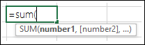
=SUM(A1:A10) is an example of a single argument.
=SUM(A1:A10, C1:C10) is an example of multiple arguments.
The following table summarizes some of the most common errors that a user can make when entering a formula, and explains how to correct them.
|
Make sure that you |
More information |
|
Start every function with the equal sign (=) |
If you omit the equal sign, what you type may be displayed as text or as a date. For example, if you type SUM(A1:A10), Excel displays the text string SUM(A1:A10) and does not perform the calculation. If you type 11/2, Excel displays the date 2-Nov (assuming the cell format is General) instead of dividing 11 by 2. |
|
Match all open and closing parentheses |
Make sure that all parentheses are part of a matching pair (opening and closing). When you use a function in a formula, it is important for each parenthesis to be in its correct position for the function to work correctly. For example, the formula =IF(B5<0),»Not valid»,B5*1.05) will not work because there are two closing parentheses and only one open parenthesis, when there should only be one each. The formula should look like this: =IF(B5<0,»Not valid»,B5*1.05). |
|
Use a colon to indicate a range |
When you refer to a range of cells, use a colon (:) to separate the reference to the first cell in the range and the reference to the last cell in the range. For example, =SUM(A1:A5), not =SUM(A1 A5), which would return a #NULL! Error. |
|
Enter all required arguments |
Some functions have required arguments. Also, make sure that you have not entered too many arguments. |
|
Enter the correct type of arguments |
Some functions, such as SUM, require numerical arguments. Other functions, such as REPLACE, require a text value for at least one of their arguments. If you use the wrong type of data as an argument, Excel may return unexpected results or display an error. |
|
Nest no more than 64 functions |
You can enter, or nest, no more than 64 levels of functions within a function. |
|
Enclose other sheet names in single quotation marks |
If a formula refers to values or cells on other worksheets or workbooks, and the name of the other workbook or worksheet contains spaces or non-alphabetical characters, you must enclose its name within single quotation marks ( ‘ ), like =’Quarterly Data’!D3, or =‘123’!A1. |
|
Place an exclamation point (!) after a worksheet name when you refer to it in a formula |
For example, to return the value from cell D3 in a worksheet named Quarterly Data in the same workbook, use this formula: =’Quarterly Data’!D3. |
|
Include the path to external workbooks |
Make sure that each external reference contains a workbook name and the path to the workbook. A reference to a workbook includes the name of the workbook and must be enclosed in brackets ([Workbookname.xlsx]). The reference must also contain the name of the worksheet in the workbook. If the workbook that you want to refer to is not open in Excel, you can still include a reference to it in a formula. You provide the full path to the file, such as in the following example: =ROWS(‘C:My Documents[Q2 Operations.xlsx]Sales’!A1:A8). This formula returns the number of rows in the range that includes cells A1 through A8 in the other workbook (8). Note: If the full path contains space characters, as does the preceding example, you must enclose the path in single quotation marks (at the beginning of the path and after the name of the worksheet, before the exclamation point). |
|
Enter numbers without formatting |
Do not format numbers when you enter them in formulas. For example, if the value that you want to enter is $1,000, enter 1000 in the formula. If you enter a comma as part of a number, Excel treats it as a separator character. If you want numbers displayed so that they show thousands or millions separators, or currency symbols, format the cells after you enter the numbers. For example, if you want to add 3100 to the value in cell A3, and you enter the formula =SUM(3,100,A3), Excel adds the numbers 3 and 100 and then adds that total to the value from A3, instead of adding 3100 to A3 which would be =SUM(3100,A3). Or, if you enter the formula =ABS(-2,134), Excel displays an error because the ABS function accepts only one argument: =ABS(-2134). |
You can implement certain rules to check for errors in formulas. These rules do not guarantee that your worksheet is error free, but they can go a long way toward finding common mistakes. You can turn any of these rules on or off individually.
Errors can be marked and corrected in two ways: one error at a time (like a spell checker), or immediately when they occur on the worksheet as you enter data.
You can resolve an error by using the options that Excel displays, or you can ignore the error by clicking Ignore Error. If you ignore an error in a particular cell, the error in that cell does not appear in further error checks. However, you can reset all previously ignored errors so that they appear again.
-
For Excel on Windows, Click File > Options > Formulas, or
for Excel on Mac, click the Excel menu > Preferences > Error Checking.In Excel 2007, click the Microsoft Office button
 > Excel Options > Formulas.
 -
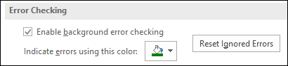
Under Error Checking, check Enable background error checking. Any error that is found, will be marked with a triangle in the top-left corner of the cell.
-
To change the color of the triangle that marks where an error occurs, in the Indicate errors using this color box, select the color that you want.
-
Under Excel checking rules, select or clear the check boxes of any of the following rules:
-
Cells containing formulas that result in an error: A formula does not use the expected syntax, arguments, or data types. Error values include #DIV/0!, #N/A, #NAME?, #NULL!, #NUM!, #REF!, and #VALUE!. Each of these error values have different causes and are resolved in different ways.
Note: If you enter an error value directly in a cell, it is stored as that error value but is not marked as an error. However, if a formula in another cell refers to that cell, the formula returns the error value from that cell.
-
Inconsistent calculated column formula in tables: A calculated column can include individual formulas that are different from the master column formula, which creates an exception. Calculated column exceptions are created when you do any of the following:
-
Type data other than a formula in a calculated column cell.
-
Type a formula in a calculated column cell, and then use Ctrl +Z or click Undo
on the Quick Access Toolbar. -
Type a new formula in a calculated column that already contains one or more exceptions.
-
Copy data into the calculated column that does not match the calculated column formula. If the copied data contains a formula, this formula overwrites the data in the calculated column.
-
Move or delete a cell on another worksheet area that is referenced by one of the rows in a calculated column.
-
-
Cells containing years represented as 2 digits: The cell contains a text date that can be misinterpreted as the wrong century when it is used in formulas. For example, the date in the formula =YEAR(«1/1/31») could be 1931 or 2031. Use this rule to check for ambiguous text dates.
-
Numbers formatted as text or preceded by an apostrophe: The cell contains numbers stored as text. This typically occurs when data is imported from other sources. Numbers that are stored as text can cause unexpected sorting results, so it is best to convert them to numbers. ‘=SUM(A1:A10) is seen as text.
-
Formulas inconsistent with other formulas in the region: The formula does not match the pattern of other formulas near it. In many cases, formulas that are adjacent to other formulas differ only in the references used. In the following example of four adjacent formulas, Excel displays an error next to the formula =SUM(A10:C10) in cell D4 because the adjacent formulas increment by one row, and that one increments by 8 rows — Excel expects the formula =SUM(A4:C4).
If the references that are used in a formula are not consistent with those in the adjacent formulas, Excel displays an error.
-
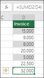
Formulas which omit cells in a region: A formula may not automatically include references to data that you insert between the original range of data and the cell that contains the formula. This rule compares the reference in a formula against the actual range of cells that is adjacent to the cell that contains the formula. If the adjacent cells contain additional values and are not blank, Excel displays an error next to the formula.
For example, Excel inserts an error next to the formula =SUM(D2:D4) when this rule is applied, because cells D5, D6, and D7 are adjacent to the cells that are referenced in the formula and the cell that contains the formula (D8), and those cells contain data that should have been referenced in the formula.
-
Unlocked cells containing formulas: The formula is not locked for protection. By default, all cells on a worksheet are locked so they can’t be changed when the worksheet is protected. This can help avoid inadvertent mistakes like accidentally deleting or altering formulas. This error indicates that the cell has been set to be unlocked, but the sheet has not been protected. Check to make sure that you do not want the cell locked or not.
-
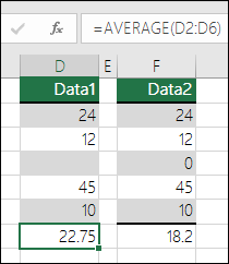
Formulas referring to empty cells: The formula contains a reference to an empty cell. This can cause unintended results, as shown in the following example.
Suppose you want to calculate the average of the numbers in the following column of cells. If the third cell is blank, it is not included in the calculation and the result is 22.75. If the third cell contains 0, the result is 18.2.
-
Data entered in a table is invalid: There is a validation error in a table. Check the validation setting for the cell by going to the Data tab > Data Tools group > Data Validation.
-
 > Excel Options > Formulas.
 on the Quick Access Toolbar.
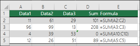
-
Select the worksheet you want to check for errors.
-
If the worksheet is manually calculated, press F9 to recalculate.
If the Error Checking dialog is not displayed, then click on the Formulas tab > Formula Auditing > Error Checking button.
-
If you have previously ignored any errors, you can check for those errors again by doing the following: click File > Options > Formulas. For Excel on Mac, click the Excel menu > Preferences > Error Checking.
In the Error Checking section, click Reset Ignored Errors > OK.
Note: Resetting ignored errors resets all errors in all sheets in the active workbook.
Tip: It might help if you move the Error Checking dialog box just below the formula bar.
-
Click one of the action buttons in the right side of the dialog box. The available actions differ for each type of error.
-
Click Next.
Note: If you click Ignore Error, the error is marked to be ignored for each consecutive check.
-
Next to the cell, click the Error Checking button
that appears, and then click the option you want. The available commands differ for each type of error, and the first entry describes the error.If you click Ignore Error, the error is marked to be ignored for each consecutive check.
 that appears, and then click the option you want. The available commands differ for each type of error, and the first entry describes the error.
If a formula cannot correctly evaluate a result, Excel displays an error value, such as #####, #DIV/0!, #N/A, #NAME?, #NULL!, #NUM!, #REF!, and #VALUE!. Each error type has different causes, and different solutions.
The following table contains links to articles that describe these errors in detail, and a brief description to get you started.
|
Topic |
Description |
|
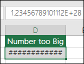
Correct a #### error |
Excel displays this error when a column is not wide enough to display all the characters in a cell, or a cell contains negative date or time values. For example, a formula that subtracts a date in the future from a date in the past, such as =06/15/2008-07/01/2008, results in a negative date value. Tip: Try to auto-fit the cell by double-clicking between the column headers. If ### is displayed because Excel can’t display all of the characters this will correct it. |
|
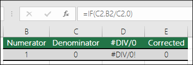
Correct a #DIV/0! error |
Excel displays this error when a number is divided either by zero (0) or by a cell that contains no value. Tip: Add an error handler like in the following example, which is =IF(C2,B2/C2,0) |
|
Correct a #N/A error |
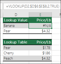
Excel displays this error when a value is not available to a function or formula. If you’re using a function like VLOOKUP, does what you’re trying to lookup have a match in the lookup range? Most often it doesn’t. Try using IFERROR to suppress the #N/A. In this case you could use: =IFERROR(VLOOKUP(D2,$D$6:$E$8,2,TRUE),0) |
|
Correct a #NAME? error |
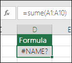
This error is displayed when Excel does not recognize text in a formula. For example, a range name or the name of a function may be spelled incorrectly. Note: If you’re using a function, make sure the function name is spelled correctly. In this case SUM is spelled incorrectly. Remove the “e” and Excel will correct it. |
|
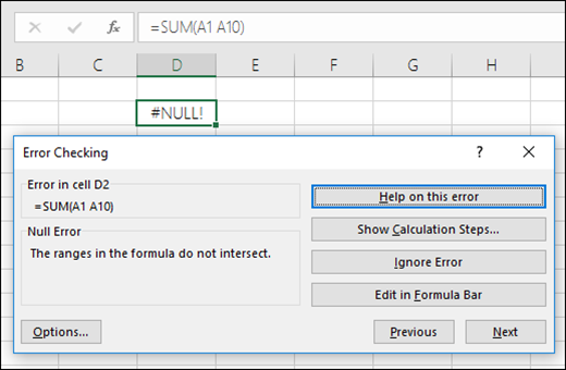
Correct a #NULL! error |
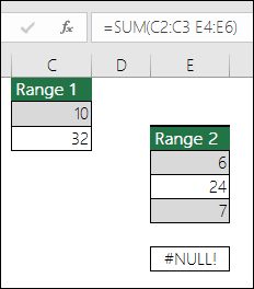
Excel displays this error when you specify an intersection of two areas that do not intersect (cross). The intersection operator is a space character that separates references in a formula. Note: Make sure your ranges are correctly separated — the areas C2:C3 and E4:E6 do not intersect, so entering the formula =SUM(C2:C3 E4:E6) returns the #NULL! error. Putting a comma between the C and E ranges will correct it =SUM(C2:C3,E4:E6) |
|
Correct a #NUM! error |
Excel displays this error when a formula or function contains invalid numeric values. Are you using a function that iterates, such as IRR or RATE? If so, the #NUM! error is probably because the function can’t find a result. Refer to the help topic for resolution steps. |
|
Correct a #REF! error |
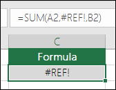
Excel displays this error when a cell reference is not valid. For example, you may have deleted cells that were referred to by other formulas, or you may have pasted cells that you moved on top of cells that were referred to by other formulas. Did you accidentally delete a row or column? We deleted column B in this formula, =SUM(A2,B2,C2), and look what happened. Either use Undo (Ctrl+Z) to undo the deletion, rebuild the formula, or use a continuous range reference like this: =SUM(A2:C2), which would have automatically updated when column B was deleted. |
|
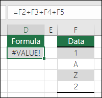
Correct a #VALUE! error |
Excel can display this error if your formula includes cells that contain different data types. Are you using Math operators (+, -, *, /, ^) with different data types? If so, try using a function instead. In this case =SUM(F2:F5) would correct the problem. |
When cells are not visible on a worksheet, you can watch those cells and their formulas in the Watch Window toolbar. The Watch Window makes it convenient to inspect, audit, or confirm formula calculations and results in large worksheets. By using the Watch Window, you don’t need to repeatedly scroll or go to different parts of your worksheet.
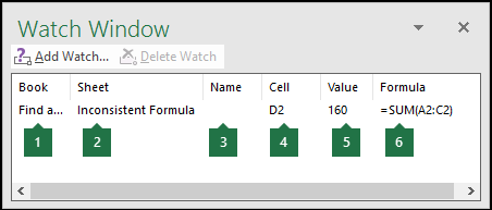
This toolbar can be moved or docked like any other toolbar. For example, you can dock it on the bottom of the window. The toolbar keeps track of the following cell properties: 1) Workbook, 2) Sheet, 3) Name (if the cell has a corresponding Named Range), 4) Cell address, 5) Value, and 6) Formula.
Note: You can have only one watch per cell.
Add cells to the Watch Window
-
Select the cells that you want to watch.
To select all cells on a worksheet with formulas, on the Home tab, in the Editing group, click Find & Select (or you can use Ctrl+G, or Control+G on the Mac)> Go To Special > Formulas.
-
On the Formulas tab, in the Formula Auditing group, click Watch Window.
-
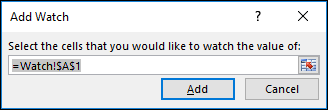
Click Add Watch.
-
Confirm that you have selected all of the cells you want to watch and click Add.
-
To change the width of a Watch Window column, drag the boundary on the right side of the column heading.
-
To display the cell that an entry in Watch Window toolbar refers to, double-click the entry.
Note: Cells that have external references to other workbooks are displayed in the Watch Window toolbar only when the other workbooks are open.


Remove cells from the Watch Window
-
If the Watch Window toolbar is not displayed, on the Formulas tab, in the Formula Auditing group, click Watch Window.
-
Select the cells that you want to remove.
To select multiple cells, press CTRL and then click the cells.
-
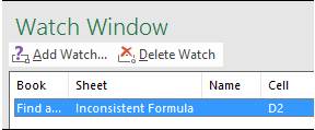
Click Delete Watch.
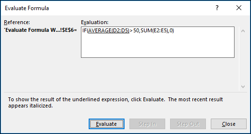
Sometimes, understanding how a nested formula calculates the final result is difficult because there are several intermediate calculations and logical tests. However, by using the Evaluate Formula dialog box, you can see the different parts of a nested formula evaluated in the order the formula is calculated. For example, the formula =IF(AVERAGE(D2:D5)>50,SUM(E2:E5),0)is easier to understand when you can see the following intermediate results:
|
In the Evaluate Formula dialog box |
Description |
|
=IF(AVERAGE(D2:D5)>50,SUM(E2:E5),0) |
The nested formula is initially displayed. The AVERAGE function and the SUM function are nested within the IF function. The cell range D2:D5 contains the values 55, 35, 45, and 25, and so the result of the AVERAGE(D2:D5) function is 40. |
|
=IF(40>50,SUM(E2:E5),0) |
The cell range D2:D5 contains the values 55, 35, 45, and 25, and so the result of the AVERAGE(D2:D5) function is 40. |
|
=IF(False,SUM(E2:E5),0) |
Because 40 is not greater than 50, the expression in the first argument of the IF function (the logical_test argument) is False. The IF function returns the value of the third argument (the value_if_false argument). The SUM function is not evaluated because it is the second argument to the IF function (value_if_true argument), and it is returned only when the expression is True. |
-
Select the cell that you want to evaluate. Only one cell can be evaluated at a time.
-
Select the Formulas tab > Formula Auditing > Evaluate Formula.
-
Click Evaluate to examine the value of the underlined reference. The result of the evaluation is shown in italics.
If the underlined part of the formula is a reference to another formula, click Step In to display the other formula in the Evaluation box. Click Step Out to go back to the previous cell and formula.
The Step In button is not available for a reference the second time the reference appears in the formula, or if the formula refers to a cell in a separate workbook.
-
Continue clicking Evaluate until each part of the formula has been evaluated.
-
To see the evaluation again, click Restart.
-
To end the evaluation, click Close.
Notes:
-
Some parts of formulas that use the IF and CHOOSE functions are not evaluated — in these cases, #N/A is displayed in the Evaluation box.
-
If a reference is blank, a zero value (0) is displayed in the Evaluation box.
-
The following functions are recalculated each time the worksheet changes, and can cause the Evaluate Formula dialog box to give results different from what appears in the cell: RAND, AREAS, INDEX, OFFSET, CELL, INDIRECT, ROWS, COLUMNS, NOW, TODAY, RANDBETWEEN.
Need more help?

You can always ask an expert in the Excel Tech Community or get support in the Answers community.
See Also
Display the relationships between formulas and cells
How to avoid broken formulas
Need more help?
Want more options?
Explore subscription benefits, browse training courses, learn how to secure your device, and more.
Communities help you ask and answer questions, give feedback, and hear from experts with rich knowledge.
Errors are quite common. You will not find a single person who does not make any errors in Excel. When the errors are part and parcel of Excel, one must know how to find those errors and resolve those issues.
When using Excel routinely, we may encounter many errors flagged if the error handler is enabled. Otherwise, we may get potential calculation errors. So if you are new to error handling in Excel, this article is a perfect guide for you.
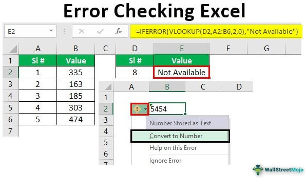
Table of contents
- How to Find Errors in Excel?
- Find and Handle Errors in Excel
- Example #1 – Error Handling through Error Handler
- Example #2 – Formulas Error Handling
- Things to Remember
- Recommended Articles
- Find and Handle Errors in Excel
Find and Handle Errors in Excel
You can download this Error Checking Excel Template here – Error Checking Excel Template
Whenever an Excel cell encounters an error, it will, by default, display the error through the error handler. The error handler in Excel is a built-in tool. We can enable this using this and get the full benefit of it.
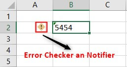
As we can see in the above image, we have an error notifier showing that there is an error with the cell B2 value.
You also must have come across this error handler in Excel but are not aware of this. If the Excel worksheet does not show this error handling message, we must enable this by following the below steps:
- We must first click on the “File” tab in the ribbon.

- Under the “File” tab, click on “Options.”

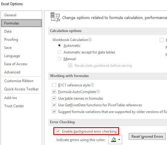
- It will open the “Excel Options” window. Next, click on the “Formulas” tab.

- Under “Error Checking,” check the “Enable background error checking” box.

At the bottom, we can choose the color which can notify the error. The green color has been selected by default, but we can change this.


Example #1 – Error Handling through Error Handler
When the data format is not proper, we may get errors. So in those scenarios, in that particular cell, we may see that error notification.
- For example, look at the below image of an error.
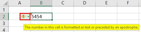
When we place our cursor on that error handler, it shows the message, “The number in this cell is formatted as text or preceded by an apostrophe.”
- To fix this error, we must click on the drop-down listA drop-down list in excel is a pre-defined list of inputs that allows users to select an option.read more of the icon, and we see the below options.
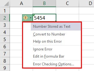
- The first displays “Number Stored as Text,” which is the error. To fix this excel errorErrors in excel are common and often occur at times of applying formulas. The list of nine most common excel errors are — #DIV/0, #N/A, #NAME?, #NULL!, #NUM!, #REF!, #VALUE!, #####, Circular Reference.read more, look at the second option. The “Convert to Number” mentions clicking on these options. Therefore, it will solve the error.
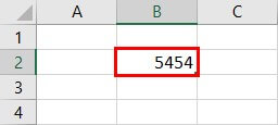
Now, look at the cell. It has no error message icon now. Like this, we can fix data format-related errors easily.
Example #2 – Formulas Error Handling
Formulas often return an error. To deal with those errors, we need to employ a different strategy. Before handling the error, we need to look at the kind of errors we encounter in different scenarios.
Below are the kind of errors we see in Excel.
- #DIV/0! – If the number is divided by 0 or an empty cell, we may get the #DIV/0 error#DIV/0! is the division error in Excel which occurs every time a number is divided by zero. Simply put, we get this error when we divide any number by an empty or zero-value cell.read more.
- #N/A – If the VLOOKUP formula does not find a value, then we get this error.
- #NAME? – If the formula name is not recognized, we get this error.
- #REF! – When the formula reference cell is deleted, or the formula reference area is out of range, we may get this #REF! Error.
- #VALUE! – When wrong data types are included in the formula, we may get the #VALUE! Error#VALUE! Error in Excel represents that the reference cell the user has either entered an incorrect formula or used a wrong data type (mostly numerical data). Sometimes, it is difficult to identify the kind of mistake behind this error.read more.
So, to deal with the above error values, we need to use the IFERROR functionThe IFERROR function in Excel checks a formula (or a cell) for errors and returns a specified value in place of the error.read more.
- For example, look at the below formula image.
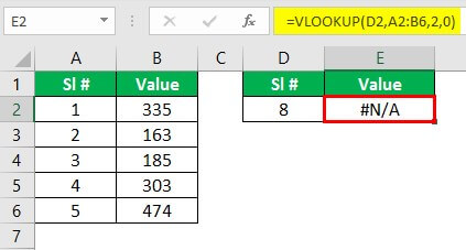
The VLOOKUP formula has been applied. However, the LOOKUP value “8” is not mentioned in the “Table Array” range A2 to B6, so the VLOOKUP returns an error value as #N/A, i.e., not available error.
- To fix this error, we must use the IFERROR function.
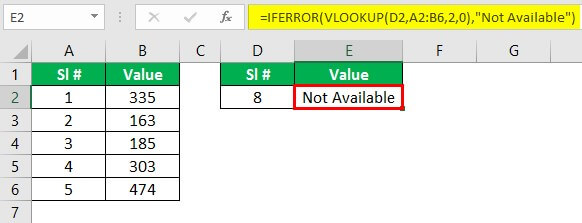
Before using the VLOOKUP function, we used the IFERROR function. If the VLOOKUP function returns an error instead of a result, the IFERROR function returns the alternative outcome, “Not Available,” instead of the traditional #N/A error result.
Like this, we can handle errors in Excel.
Things to Remember
- The error notifier will show an error icon if the cell value data type is unsuitable.
- The IFERROR function is typically used to check formula errors.
Recommended Articles
This article is a guide to Finding Errors in Excel. Here, we discuss finding and handling errors in Excel, practical examples, and a downloadable Excel template. You may learn more about financing from the following articles: –
- Error Bars in Excel
- Formula Errors in Excel
- IFERROR with VLOOKUP in Excel
- Excel Test
See all How-To Articles
This tutorial will demonstrate how to use Error Checking in Excel and Google Sheets.
Background Error Checking
Errors in Excel formulas usually show up as a small green triangle in the top left-hand corner of a cell. If you click in the cell that contains an error, a drop down list is enabled from which you can select the option you require.
If the background error checking options are not switched on in Excel, then this triangle will not show up, but the cell will still contain an error value.
In order to ensure you see the triangle, which makes error checking easier, make sure background checking is switched on in Excel options.
1. In the Ribbon, select File. Then select Options > Formulas.
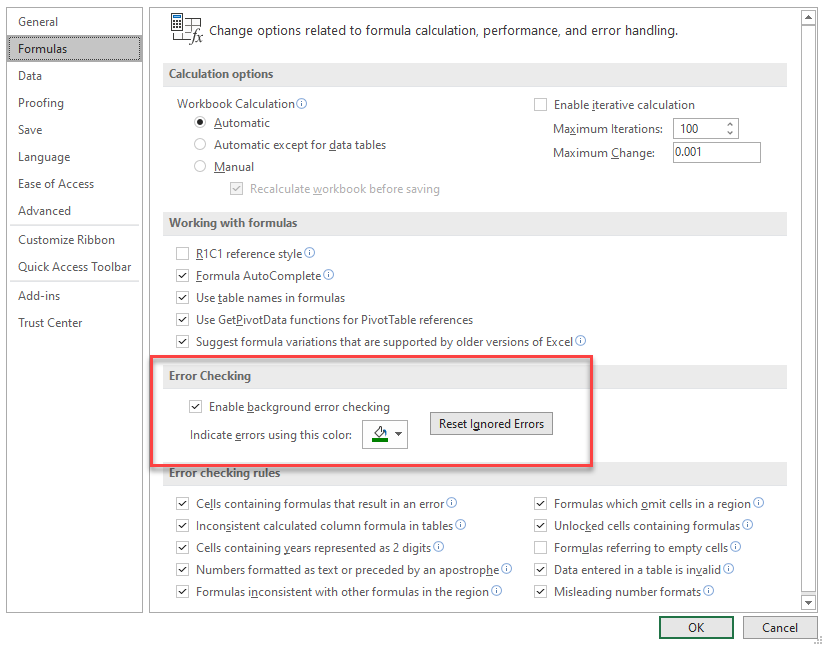
2. Make sure the check-mark “Enable background error checking” is checked and then click OK. (Usually, this is already checked by default in Excel.)
How to Use Error Checking
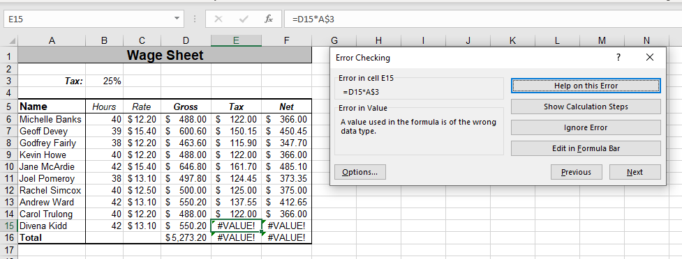
1. With the file that contains the errors open in Excel, in the Ribbon, select Formula > Formula Auditing > Error Checking.

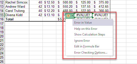
2. In the Error Checking dialog box, click Show Calculation Steps.
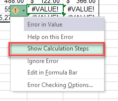
OR
Click on the small green triangle in the left-hand side of the cell that contains the error, and select Show Calculation Steps.
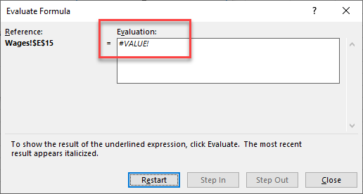
3. Click Evaluate to evaluate the error.
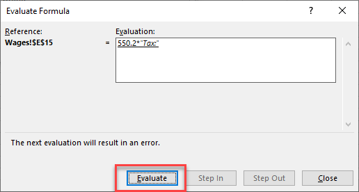
4. Keep clicking evaluate until you get the message: “The next evaluation will result in an error.”
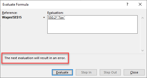
The error is shown in the formula in the dialog box.
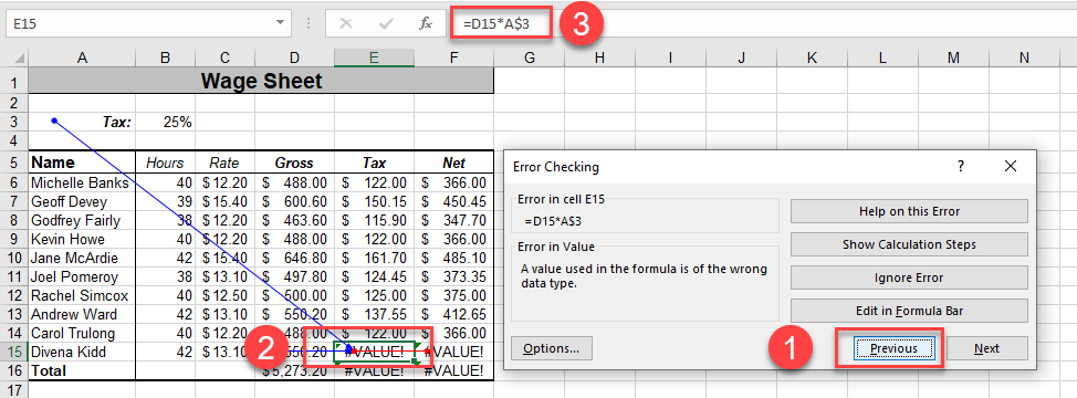
5. Click Close, and then (1) click Next to move to the next error. Then (2) click Trace to trace the error.
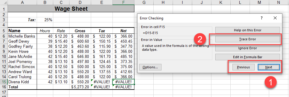
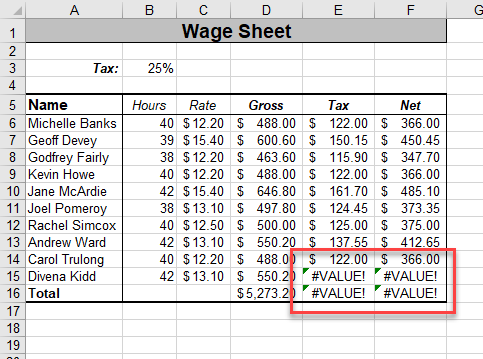
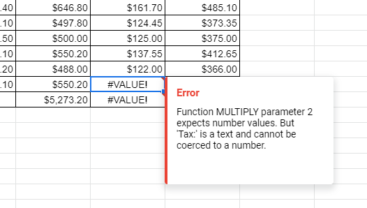
Excel will highlight the error with tracing arrows allowing you to see where the error is originating from. In this case, the #VALUE in the error is coming from the #VALUE in the previous error but the formula in the formula bar looks fine.
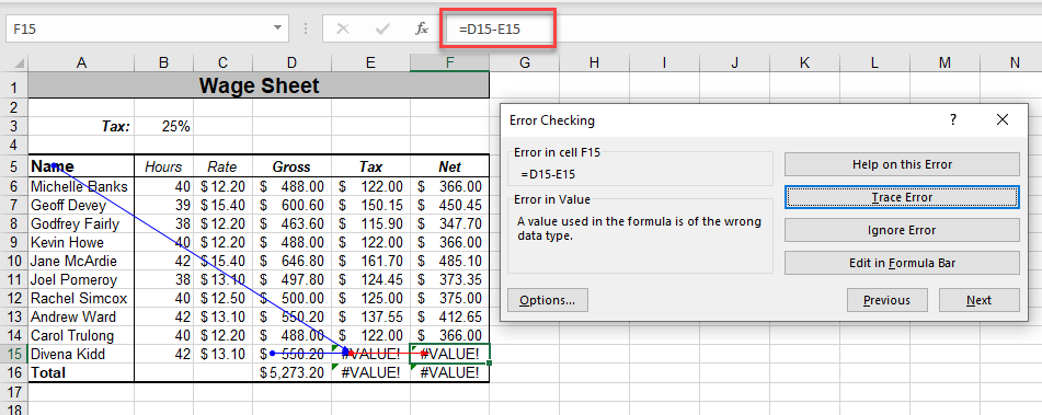
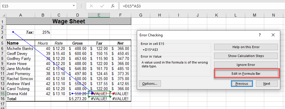
6. Click (1) Previous to move to the previous error. The cell pointer will in this case (2) move to E15. The formula in E15 is shown (3) in the formula bar. Here, you can see that the formula is multiplying a value (e.g., in D15) with text (e.g., in A3).
7. Click Edit in Formula bar.
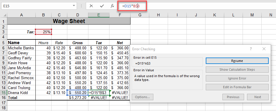
8. Amend the formula as appropriate, and then click Resume.
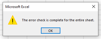
If all the errors in the worksheet are fixed, Error Checking will stop.
This example showed #VALUE errors, but Error Checking will find all # errors. There is a different option for circular references.
Error Checking in Google Sheets
Error checking is automatic in Google Sheets. As soon as you have a cell that contains an error, it will show up on the screen with details about the error.
 In this Excel IFERROR, ISERROR, ISERR, IFNA and ISNA Tutorial, you learn how to use the IFERROR, ISERROR, ISERR, IFNA and ISNA functions in your worksheet formulas for the following:
- Identify errors, including the #N/A error.
- Handle errors, including the #N/A error, and return a specific:
- Value;
- Formula;
- Expression; or
- Reference.
- Carry out VLookups that handle errors, including the #N/A error, and return a specific:
- Value;
- Formula;
- Expression; or
- Reference.
- Check whether a specific value exists in a list or compare 2 columns.
This Excel IFERROR, ISERROR, ISERR, IFNA and ISNA Tutorial is accompanied by an Excel workbook containing the data and formulas I use in the examples below. You can get immediate free access to this example workbook by subscribing to the Power Spreadsheets Newsletter.
Use the following Table of Contents to navigate to the section you’re interested in.
Related Excel Tutorials
The following Tutorials may help you better understand and implement the contents below:
- Formulas and functions:
- Learn how to work with the LEFT, RIGHT, MID, LEN, FIND and SEARCH functions here.
- Macros and VBA:
- Learn how to use worksheet functions in macros here.
- Learn how to work with the VLookup function in VBA here.
You can find additional Tutorials in the Archives.
IFERROR formula
To handle possible errors with the IFERROR function, use a formula with the following structure:
=IFERROR(Value,ValueIfError)
IFERROR process
To handle possible errors with the IFERROR function, follow these steps:
- Specify the expression you want to check for errors (Value).
- Specify that, if Value returns an error (IFERROR), another value (ValueIfError) is returned.
IFERROR formula explanation
Item: IFERROR
The IFERROR function:
- Returns the value you specify (ValueIfError) if an expression (Value) returns an error; and
- Returns the result of that expression (Value) otherwise.
In other words, IFERROR does the following:
- Checks an expression (Value).
- If Value returns an error, IFERROR returns the value you specify (ValueIfError).
- If Value doesn’t return an error, IFERROR returns the result of that expression.
Therefore, you usually use IFERROR to trap and handle errors in worksheet formulas. The IFERROR function deals with the following errors:
- #N/A.
- #VALUE!
- #REF!
- #DIV/0!
- #NUM!
- #NAME?
- #NULL!
Item: Value
The value argument of the IFERROR function (Value) is a value, formula, expression or reference that Excel checks for errors.
If Value doesn’t return an error, IFERROR returns the result of that expression.
Item: ValueIfError
The value_if_error argument of the IFERROR function (ValueIfError) is the value, formula, expression or reference that Excel returns if the value argument of the IFERROR function (Value) evaluates to an error.
IFERROR formula example
The worksheet formulas below handle possible errors with the IFERROR function, as follows:
- Value: The quotient obtained by dividing:
- The value specified in column G (G12 to G16); by
- The value specified in column F (F12 to F16).
- ValueIfError: The string “Total Sales are $ 0” (“Total Sales are $ 0”).
| No. | IFERROR formula |
| 1 | =IFERROR(G12/F12,"Total Sales are $ 0") |
| 2 | =IFERROR(G13/F13,"Total Sales are $ 0") |
| 3 | =IFERROR(G14/F14,"Total Sales are $ 0") |
| 4 | =IFERROR(G15/F15,"Total Sales are $ 0") |
| 5 | =IFERROR(G16/F16,"Total Sales are $ 0") |
Effects of using IFERROR formula example
The following image illustrates the results returned by the IFERROR formula that handles possible errors. As expected, the formulas (in cells H12 to H16):
- Check an expression (Value) for errors; and
- Return the following:
- If Value returns an error: The string “Total Sales are $ 0” (ValueIfError).
- If Value doesn’t return an error: Value itself.
Notice the difference between the result returned by the IFERROR formula that handles errors in cell H16 and the result returned by the regular formula (without IFERROR) in cell H11.

#2: IFERROR then 0
IFERROR then 0 formula
To return 0 if an expression returns an error (with the IFERROR function), use a formula with the following structure:
IFERROR then 0 process
To return 0 if an expression returns an error (with the IFERROR function), follow these steps:
- Specify the expression you want to check for errors (Value).
- Specify that, if Value returns an error (IFERROR), 0 (0) is returned.
IFERROR then 0 formula explanation
Item: IFERROR
The IFERROR function:
- Returns the value you specify (0) if an expression (Value) returns an error; and
- Returns the result of that expression (Value) otherwise.
In other words, IFERROR does the following:
- Checks an expression (Value).
- If Value returns an error, IFERROR returns the value you specify (0).
- If Value doesn’t return an error, IFERROR returns the result of that expression.
Therefore, you usually use IFERROR to trap and handle errors in worksheet formulas. The IFERROR function deals with the following errors:
- #N/A.
- #VALUE!
- #REF!
- #DIV/0!
- #NUM!
- #NAME?
- #NULL!
Item: Value
The value argument of the IFERROR function (Value) is a value, formula, expression or reference that Excel checks for errors.
If Value doesn’t return an error, IFERROR returns the result of that expression.
Item: 0
The value_if_error argument of the IFERROR function (0) is the value, formula, expression or reference that Excel returns if the value argument of the IFERROR function (Value) evaluates to an error.
To return 0 if an expression (Value) returns an error, set value_if_error to 0.
IFERROR then 0 formula example
The worksheet formulas below return 0 if an expression returns an error (with the IFERROR function), where Value is the quotient obtained by dividing:
- The value specified in column G (G22 to G26); by
- The value specified in column F (F22 to F26).
| No. | IFERROR then 0 formula |
| 1 | =IFERROR(G22/F22,0) |
| 2 | =IFERROR(G23/F23,0) |
| 3 | =IFERROR(G24/F24,0) |
| 4 | =IFERROR(G25/F25,0) |
| 5 | =IFERROR(G26/F26,0) |
Effects of using IFERROR then 0 formula example
The following image illustrates the results returned by the IFERROR formula that handles possible errors by returning 0. As expected, the formulas (in cells H22 to H26):
- Check an expression (Value) for errors; and
- Return the following:
- If Value returns an error: 0.
- If Value doesn’t return an error: Value itself.
Notice the difference between the result returned by the IFERROR formula that handles errors by returning 0 in cell H26 and the result returned by the regular formula (without IFERROR then 0) in cell H21.

#3: IFERROR then blank
IFERROR then blank formula
To return a blank if an expression returns an error (with the IFERROR function), use a formula with the following structure:
IFERROR then blank process
To return a blank if an expression returns an error (with the IFERROR function), follow these steps:
- Specify the expression you want to check for errors (Value).
- Specify that, if Value returns an error (IFERROR), a zero-length string (“”) is returned.
IFERROR then blank formula explanation
Item: IFERROR
The IFERROR function:
- Returns the value you specify (“”) if an expression (Value) returns an error; and
- Returns the result of that expression (Value) otherwise.
In other words, IFERROR does the following:
- Checks an expression (Value).
- If Value returns an error, IFERROR returns the value you specify (“”).
- If Value doesn’t return an error, IFERROR returns the result of that expression.
Therefore, you usually use IFERROR to trap and handle errors in worksheet formulas. The IFERROR function deals with the following errors:
- #N/A.
- #VALUE!
- #REF!
- #DIV/0!
- #NUM!
- #NAME?
- #NULL!
Item: Value
The value argument of the IFERROR function (Value) is a value, formula, expression or reference that Excel checks for errors.
If Value doesn’t return an error, IFERROR returns the result of that expression.
Item: “”
The value_if_error argument of the IFERROR function (“”) is the value, formula, expression or reference that Excel returns if the value argument of the IFERROR function (Value) evaluates to an error.
To return a blank if an expression (Value) returns an error, set value_if_error to a zero-length string (“”).
IFERROR then blank formula example
The worksheet formulas below return a blank if an expression returns an error (with the IFERROR function), where Value is the quotient obtained by dividing:
- The value specified in column G (G32 to G36); by
- The value specified in column F (F32 to F36).
| No. | IFERROR then blank formula |
| 1 | =IFERROR(G32/F32,"") |
| 2 | =IFERROR(G33/F33,"") |
| 3 | =IFERROR(G34/F34,"") |
| 4 | =IFERROR(G35/F35,"") |
| 5 | =IFERROR(G36/F36,"") |
Effects of using IFERROR then blank formula example
The following image illustrates the results returned by the IFERROR formula that handles possible errors by returning a blank (“”). As expected, the formulas (in cells H32 to H36):
- Check an expression (Value) for errors; and
- Return the following:
- If Value returns an error: A zero-length string (“”).
- If Value doesn’t return an error: Value itself.
Notice the difference between the result returned by the IFERROR formula that handles errors by returning a blank in cell H36 and the result returned by the regular formula (without IFERROR then blank) in cell H31.

#4: IFERROR VLOOKUP
IFERROR VLOOKUP formula
To carry out a VLookup that handles possible errors (with IFERROR vs. IFNA), use a formula with the following structure:
=IFERROR(VLOOKUP(LookupValue,LookupTable,ColumnIndex,RangeLookup),ValueIfError)
IFERROR VLOOKUP process
To carry out a VLookup that handles possible errors (with IFERROR vs. IFNA), follow these steps:
- Specify the value you want to look up (LookupValue) in the first (leftmost) column of a table (LookupTable).
- Identify the cell range (a table array) containing the lookup table (LookupTable).
- Specify the index number of the column (within LookupTable) from which you want to obtain a value (ColumnIndex).
- Specify whether VLOOKUP searches for an exact or approximate match (RangeLookup).
- Specify that, if VLOOKUP returns an error (IFERROR), another value (ValueIfError) is returned.
IFERROR VLOOKUP formula explanation
Formula #1: VLOOKUP(LookupValue,LookupTable,ColumnIndex,RangeLookup)
Item: VLOOKUP
The VLOOKUP function does the following:
- Looks for a value (LookupValue) in the first (leftmost) column of a table (LookupTable); and
- Returns a value in the same row but from another column you specify (ColumnIndex).
Item: LookupValue
The lookup_value argument of the VLOOKUP function (LookupValue) is the value you look up in the first (leftmost) column of LookupTable. In other words, LookupValue must usually be in the first column of the cell range you specify as LookupTable.
If VLOOKUP doesn’t find LookupValue in the first column of LookupTable, it usually returns the #N/A error.
You can specify LookupValue as either:
- A value;
- A text string; or
- A cell reference.
Item: LookupTable
The table_array argument of the VLOOKUP function (LookupTable) is the cell range in which VLOOKUP searches for the following:
- The LookupValue in the first column of LookupTable; and
- The value to return in the column you specify (ColumnIndex).
Therefore, the cell range you specify as LookupTable must usually include both of the following columns:
- The first column, which must contain the LookupValue; and
- The column from which VLOOKUP should return a value.
If VLOOKUP doesn’t find LookupValue in the first column of LookupTable, it usually returns the #N/A error.
Item: ColumnIndex
The col_index_num argument of the VLOOKUP function (ColumnIndex) is the column number within the LookupTable from which VLOOKUP returns a value, as follows:
| Column | ColumnIndex | Comments |
| First | 1 | Must usually contain the LookupValue. Otherwise, VLOOKUP usually returns the #N/A error. |
| Second | 2 | |
| Third | 3 | |
| … | … | |
| #th | # |
Item: RangeLookup
The range_lookup argument of the VLOOKUP function (RangeLookup) specifies whether VLOOKUP searches for an approximate or an exact match for LookupValue in the first column of LookupTable.
- Set RangeLookup to TRUE when searching for an approximate match.
- Set RangeLookup to FALSE when searching for an exact match.
Formula #2: IFERROR(VLOOKUP(…),ValueIfError)
Item: IFERROR
The IFERROR function:
- Returns the value you specify (ValueIfError) if an expression (VLOOKUP(…)) returns an error; and
- Returns the result of that expression (VLOOKUP(…)) otherwise.
In other words, IFERROR does the following:
- Checks an expression (VLOOKUP(…)).
- If VLOOKUP(…) returns an error, IFERROR returns the value you specify (ValueIfError).
- If VLOOKUP(…) doesn’t return an error, IFERROR returns the result of that formula.
Item: VLOOKUP(…)
The value argument of the IFERROR function (VLOOKUP(…)) is a value, formula, expression or reference that Excel checks for errors.
If VLOOKUP(….) doesn’t return an error, IFERROR returns the result of that formula. For the explanation of this VLOOKUP function, please refer to the appropriate section in this Tutorial.
One of the most common errors returned by the VLOOKUP function is #N/A. The VLOOKUP function usually returns an #N/A error when you either:
- Give an inappropriate value (including a value that isn’t found in the first column of LookupTable) for the lookup_value argument (LookupValue); or
- Use the function to locate a value in a table (LookupTable) that isn’t properly sorted.
Item: ValueIfError
The value_if_error argument of the IFERROR function (ValueIfError) is the value, formula, expression or reference that Excel returns if the value argument of the IFERROR function (VLOOKUP(…)) evaluates to an error.
IFERROR VLOOKUP formula example
The worksheet formula below carries out an exact match VLookup and handles possible errors (with IFERROR vs. IFNA), as follows:
- LookupValue: The value specified in cell M8 ($M$8).
- LookupTable: The lookup table in cells A8 to E57 ($A$8:$E$57).
- ColumnIndex: The column number specified in column K (K10).
- RangeLookup: FALSE.
- ValueIfError: The string “Sales Manager not found” (“Sales Manager not found”).
=IFERROR(VLOOKUP($M$8,$A$8:$E$57,K10,FALSE),"Sales Manager not found")
Effects of using IFERROR VLOOKUP formula example
The following images illustrate the results returned by the IFERROR VLOOKUP formula that carries out a VLookup that handles possible errors (with IFERROR vs. IFNA).
The image below displays the LookupTable.

The image below displays the results returned by IFERROR VLOOKUP. As expected, the formula in cell M10 does the following:
- Looks for the value (LookupValue) specified in cell M8 (Shawn Brooks) in the first column (column A) of the lookup table (LookupTable).
- The LookupValue (Shawn Brooks) isn’t found in the first column of LookupTable. Therefore, the IFERROR VLOOKUP formula returns “Sales Manager not found”.
Notice the difference between the result returned by the IFERROR VLOOKUP formula that handles errors (cell M10) and the result returned by the regular VLOOKUP formula in cell M9 (#N/A).
")
#5: ISERROR
ISERROR formula
To check whether an expression returns an error (with the ISERROR function), use a formula with the following structure:
ISERROR process
To check whether an expression returns an error (with the ISERROR function), specify the expression you want to check for errors (Value).
ISERROR formula explanation
Item: ISERROR
The ISERROR function:
- Tests whether an expression (Value) returns an error; and
- Returns:
- TRUE if Value returns an error; or
- FALSE otherwise.
The ISERROR function identifies the following errors:
- #N/A.
- #VALUE!
- #REF!
- #DIV/0!
- #NUM!
- #NAME?
- #NULL!
Item: Value
The value argument of the ISERROR function (Value) is a value, formula, expression or reference that Excel checks for errors.
ISERROR formula example
The worksheet formulas below check whether an expression returns an error (with the ISERROR function), where Value is the quotient obtained by dividing:
- The value specified in column G (G42 to G46); by
- The value specified in column F (F42 to F46).
| No. | ISERROR formula |
| 1 | =ISERROR(G42/F42) |
| 2 | =ISERROR(G43/F43) |
| 3 | =ISERROR(G44/F44) |
| 4 | =ISERROR(G45/F45) |
| 5 | =ISERROR(G46/F46) |
Effects of using ISERROR formula example
The following image illustrates the results returned by the ISERROR formula that checks whether an expression returns an error. As expected, the formulas (in cells H42 to H46):
- Check an expression (Value) for errors; and
- Return the following:
- TRUE: If Value returns an error.
- FALSE: If Value doesn’t return an error.
Notice the difference between the result returned by the ISERROR formula that checks whether an expression returns an error in cell H46 and the result returned by the regular formula (without ISERROR) in cell H41.

#6: IF ISERROR
IF ISERROR formula
To handle possible errors (with IF ISERROR vs. IFERROR), use a formula with the following structure:
=IF(ISERROR(Value),ValueIfError,Value)
IF ISERROR process
To handle possible errors (with IF ISERROR vs. IFERROR), follow these steps:
- Specify the expression you want to check for errors (Value).
- Test whether Value returns an error (ISERROR) and specify (IF) that:
- If Value returns an error, another value (ValueIfError) is returned; and
- If Value doesn’t return an error, Value itself is returned.
IF ISERROR formula explanation
Formula #1: ISERROR(Value)
Item: ISERROR
The ISERROR function:
- Tests whether an expression (Value) returns an error; and
- Returns:
- TRUE if Value returns an error; or
- FALSE otherwise.
The ISERROR function identifies the following errors:
- #N/A.
- #VALUE!
- #REF!
- #DIV/0!
- #NUM!
- #NAME?
- #NULL!
Item: Value
The value argument of the ISERROR function (Value) is a value, formula, expression or reference that Excel checks for errors.
If Value doesn’t return an error, IF returns the result of that expression. For the explanation of this IF function, please refer to the appropriate section in this Tutorial.
Formula #2: IF(ISERROR(…),ValueIfError,Value)
Item: IF
The IF function:
- Tests whether a condition (ISERROR(…)) is met; and
- Returns:
- One value (ValueIfError) if the condition (ISERROR(…)) is met and returns TRUE; and
- Another value (Value) if the condition (ISERROR(…)) isn’t met and returns FALSE.
Item: ISERROR(…)
The logical_test argument of the IF function (ISERROR(…)) is the condition Excel tests and evaluates to either:
- TRUE; or
- FALSE.
For the explanation of this ISERROR function, please refer to the appropriate section in this Tutorial.
Item: ValueIfError
The value_if_true argument of the IF function (ValueIfError) is the value, formula, expression or reference that Excel returns if ISERROR(…) returns TRUE.
In other words, ValueIfError is the value, formula, expression or reference that Excel returns if the value argument of the ISERROR function (Value) returns an error.
Item: Value
The value_if_false argument of the IF function (Value) is the value, formula, expression or reference that Excel returns if ISERROR(…) returns FALSE.
In other words, Value is the value, formula, expression or reference that Excel returns if the value argument of the ISERROR function (Value itself) doesn’t return an error.
IF ISERROR formula example
The worksheet formulas below handle possible errors (with IF ISERROR vs. IFERROR), as follows:
- Value: The quotient obtained by dividing:
- The value specified in column G (G52 to G56); by
- The value specified in column F (F52 to F56).
- ValueIfError: The string “Total Sales are $ 0” (“Total Sales are $ 0”).
| No. | IF ISERROR formula |
| 1 | =IF(ISERROR(G52/F52),"Total Sales are $ 0",G52/F52) |
| 2 | =IF(ISERROR(G53/F53),"Total Sales are $ 0",G53/F53) |
| 3 | =IF(ISERROR(G54/F54),"Total Sales are $ 0",G54/F54) |
| 4 | =IF(ISERROR(G55/F55),"Total Sales are $ 0",G55/F55) |
| 5 | =IF(ISERROR(G56/F56),"Total Sales are $ 0",G56/F56) |
Effects of using IF ISERROR formula example
The following image illustrates the results returned by the IF ISERROR formula that handles possible errors (with IF ISERROR vs. IFERROR). As expected, the formulas (in cells H52 to H56):
- Check an expression (Value) for errors; and
- Return the following:
- If Value returns an error: The string “Total Sales are $ 0” (ValueIfError).
- If Value doesn’t return an error: Value itself.
Notice the difference between the result returned by the IF ISERROR formula that handles errors in cell H56 and the result returned by the regular formula (without IF ISERROR) in cell H51.
")
#7: IF ISERROR VLOOKUP
IF ISERROR VLOOKUP formula
To carry out a VLookup that handles possible errors (with IF ISERROR vs. IFERROR), use a formula with the following structure:
=IF(ISERROR(VLOOKUP(LookupValue,LookupTable,ColumnIndex,RangeLookup)),ValueIfError,VLOOKUP(LookupValue,LookupTable,ColumnIndex,RangeLookup))
IF ISERROR VLOOKUP process
To carry out a VLookup that handles possible errors (with IF ISERROR vs. IFERROR), follow these steps:
- Specify the value you want to look up (LookupValue) in the first (leftmost) column of a table (LookupTable).
- Identify the cell range (a table array) containing the lookup table (LookupTable).
- Specify the index number of the column (within LookupTable) from which you want to obtain a value (ColumnIndex).
- Specify whether VLOOKUP searches for an exact or approximate match (RangeLookup).
- Test whether VLOOKUP returns an error (ISERROR) and specify (IF) that:
- If VLOOKUP returns an error, another value (ValueIfError) is returned; and
- If VLOOKUP doesn’t return an error, the result of VLOOKUP is returned.
IF ISERROR VLOOKUP formula explanation
Formula #1: VLOOKUP(LookupValue,LookupTable,ColumnIndex,RangeLookup)
Item: VLOOKUP
The VLOOKUP function does the following:
- Looks for a value (LookupValue) in the first (leftmost) column of a table (LookupTable); and
- Returns a value in the same row but from another column you specify (ColumnIndex).
Item: LookupValue
The lookup_value argument of the VLOOKUP function (LookupValue) is the value you look up in the first (leftmost) column of LookupTable. In other words, LookupValue must usually be in the first column of the cell range you specify as LookupTable.
If VLOOKUP doesn’t find LookupValue in the first column of LookupTable, it usually returns the #N/A error.
You can specify LookupValue as either:
- A value;
- A text string; or
- A cell reference.
Item: LookupTable
The table_array argument of the VLOOKUP function (LookupTable) is the cell range in which VLOOKUP searches for the following:
- The LookupValue in the first column of LookupTable; and
- The value to return in the column you specify (ColumnIndex).
Therefore, the cell range you specify as LookupTable must usually include both of the following columns:
- The first column, which must contain the LookupValue; and
- The column from which VLOOKUP should return a value.
If VLOOKUP doesn’t find LookupValue in the first column of LookupTable, it usually returns the #N/A error.
Item: ColumnIndex
The col_index_num argument of the VLOOKUP function (ColumnIndex) is the column number within the LookupTable from which VLOOKUP returns a value, as follows:
| Column | ColumnIndex | Comments |
| First | 1 | Must usually contain the LookupValue. Otherwise, VLOOKUP usually returns the #N/A error. |
| Second | 2 | |
| Third | 3 | |
| … | … | |
| #th | # |
Item: RangeLookup
The range_lookup argument of the VLOOKUP function (RangeLookup) specifies whether VLOOKUP searches for an approximate or an exact match for LookupValue in the first column of LookupTable.
- Set RangeLookup to TRUE when searching for an approximate match.
- Set RangeLookup to FALSE when searching for an exact match.
Formula #2: ISERROR(VLOOKUP(…))
Item: ISERROR
The ISERROR function:
- Tests whether an expression (VLOOKUP(…)) returns an error; and
- Returns:
- TRUE if VLOOKUP(…) returns an error; or
- FALSE otherwise.
The ISERROR function identifies the following errors:
- #N/A.
- #VALUE!
- #REF!
- #DIV/0!
- #NUM!
- #NAME?
- #NULL!
Item: VLOOKUP(…)
The value argument of the ISERROR function (VLOOKUP(…)) is a value, formula, expression or reference that Excel checks for errors.
If VLOOKUP(…) doesn’t return an error, IF returns the result of that formula. For the explanation of these IF and VLOOKUP functions, please refer to the appropriate sections in this Tutorial.
One of the most common errors returned by the VLOOKUP function is #N/A. The VLOOKUP function usually returns an #N/A error when you either:
- Give an inappropriate value (including a value that isn’t found in the first column of LookupTable) for the lookup_value argument (LookupValue); or
- Use the function to locate a value in a table (LookupTable) that isn’t properly sorted.
Formula #3: IF(ISERROR(…),ValueIfError,VLOOKUP(…))
Item: IF
The IF function:
- Tests whether a condition (ISERROR(…)) is met; and
- Returns:
- One value (ValueIfError) if the condition (ISERROR(…)) is met and returns TRUE; and
- Another value (VLOOKUP(…)) if the condition (ISERROR(…)) isn’t met and returns FALSE.
Item: ISERROR(…)
The logical_test argument of the IF function (ISERROR(…)) is the condition Excel tests and evaluates to either:
- TRUE; or
- FALSE.
For the explanation of this ISERROR function, please refer to the appropriate section in this Tutorial.
Item: ValueIfError
The value_if_true argument of the IF function (ValueIfError) is the value, formula, expression or reference that Excel returns if ISERROR(…) returns TRUE. For the explanation of this ISERROR function, please refer to the appropriate section in this Tutorial.
Item: VLOOKUP(…)
The value_if_false argument of the IF function (VLOOKUP(…)) is the value, formula, expression or reference that Excel returns if ISERROR(…) returns FALSE.
In other words, if VLOOKUP(…) doesn’t return an error, IF returns the result of that formula. For the explanation of these IF and VLOOKUP functions, please refer to the appropriate sections in this Tutorial.
IF ISERROR VLOOKUP formula example
The worksheet formula below carries out a VLookup that handles possible errors (with IF ISERROR vs. IFERROR), as follows:
- LookupValue: The value specified in cell M8 ($M$8).
- LookupTable: The lookup table in cells A8 to E57 ($A$8:$E$57).
- ColumnIndex: The column number specified in column K (K11).
- RangeLookup: FALSE.
- ValueIfError: The string “Sales Manager not found” (“Sales Manager not found”).
=IF(ISERROR(VLOOKUP($M$8,$A$8:$E$57,K11,FALSE)),"Sales Manager not found",VLOOKUP($M$8,$A$8:$E$57,K11,FALSE))
Effects of using IF ISERROR VLOOKUP formula example
The following images illustrate the results returned by the IF ISERROR VLOOKUP formula that carries out a VLookup that handles possible errors (with IF ISERROR vs. IFERROR).
The image below displays the LookupTable.

The image below displays the results returned by IF ISERROR VLOOKUP. As expected, the formula in cell M11 does the following:
- Looks for the value (LookupValue) specified in cell M8 (Shawn Brooks) in the first column (column A) of the lookup table (LookupTable).
- The LookupValue (Shawn Brooks) isn’t found in the first column of LookupTable. Therefore, the IF ISERROR VLOOKUP formula returns “Sales Manager not found”.
Notice the difference between the result returned by the IFERROR VLOOKUP formula that handles errors (cell M11) and the result returned by the regular VLOOKUP formula in cell M9 (#N/A).
")
#8: ISERR
ISERR formula
To check whether an expression returns an error other than #N/A (with ISERR vs. ISERROR), use a formula with the following structure:
ISERR process
To check whether an expression returns an error other than #N/A (with ISERR vs. ISERROR), specify the expression (Value) you want to check for errors (other than #N/A).
ISERR formula explanation
Item: ISERR
The ISERR function:
- Tests whether an expression (Value) returns an error (other than the #N/A error); and
- Returns:
- TRUE if Value returns an error (other than the #N/A error); or
- FALSE otherwise.
The ISERR function identifies the following errors:
- #VALUE!
- #REF!
- #DIV/0!
- #NUM!
- #NAME?
- #NULL!
ISERR doesn’t identify the #N/A error.
Item: Value
The value argument of the ISERR function (Value) is a value, formula, expression or reference that Excel checks for errors (other than the #N/A error).
ISERR formula example
The worksheet formulas below check whether an expression returns an error other than #N/A (with ISERR vs. ISERROR). Value is the value specified in column H (H8 to H57) or N (N9 to N12).
| Table | No. | ISERR formula |
| 1 | 1 | =ISERR(H8) |
| 1 | 2 | =ISERR(H9) |
| 1 | 3 | =ISERR(H10) |
| 1 | 4 | =ISERR(H11) |
| 1 | 5 | =ISERR(H12) |
| 1 | … | … |
| 1 | 50 | =ISERR(H57) |
| 2 | 1 | =ISERR(N9) |
| 2 | 2 | =ISERR(N10) |
| 2 | 3 | =ISERR(N11) |
| 2 | 4 | =ISERR(N12) |
Effects of using ISERR formula example
The following images illustrate the results returned by the ISERR formula that checks whether an expression returns an error other than #N/A (with ISERR vs. ISERROR).
As expected, the formulas:
- Check an expression (Value) for errors (other than #N/A); and
- Return the following:
- TRUE: If Value returns an error other than #N/A.
- FALSE: If Value:
- Doesn’t return an error; or
- Returns #N/A.
The image below displays a table containing certain #DIV/0! errors. Notice that, when Value returns such errors (cells H12 and H22), the ISERR formula returns TRUE (cells I12 and I22).
")
The image below displays a table containing certain #N/A errors. Notice that, when Value returns such errors (cells N9 to N12), the ISERR formula continues to return FALSE (cells O9 to O12).
")
#9: IFNA VLOOKUP
IFNA VLOOKUP formula
To carry out a VLookup that handles possible #N/A errors (with IFNA vs. IFERROR), use a formula with the following structure:
=IFNA(VLOOKUP(LookupValue,LookupTable,ColumnIndex,RangeLookup),ValueIfNa)
IFNA VLOOKUP process
To carry out a VLookup that handles possible #N/A errors (with IFNA vs. IFERROR), follow these steps:
- Specify the value you want to look up (LookupValue) in the first (leftmost) column of a table (LookupTable).
- Identify the cell range (a table array) containing the lookup table (LookupTable).
- Specify the index number of the column (within LookupTable) from which you want to obtain a value (ColumnIndex).
- Specify whether VLOOKUP searches for an exact or approximate match (RangeLookup).
- Specify that, if VLOOKUP returns the #N/A error (IFNA), another value (ValueIfNa) is returned.
IFNA VLOOKUP formula explanation
Formula #1: VLOOKUP(LookupValue,LookupTable,ColumnIndex,RangeLookup)
Item: VLOOKUP
The VLOOKUP function does the following:
- Looks for a value (LookupValue) in the first (leftmost) column of a table (LookupTable); and
- Returns a value in the same row but from another column you specify (ColumnIndex).
Item: LookupValue
The lookup_value argument of the VLOOKUP function (LookupValue) is the value you look up in the first (leftmost) column of LookupTable. In other words, LookupValue must usually be in the first column of the cell range you specify as LookupTable.
If VLOOKUP doesn’t find LookupValue in the first column of LookupTable, it usually returns the #N/A error.
You can specify LookupValue as either:
- A value;
- A text string; or
- A cell reference.
Item: LookupTable
The table_array argument of the VLOOKUP function (LookupTable) is the cell range in which VLOOKUP searches for the following:
- The LookupValue in the first column of LookupTable; and
- The value to return in the column you specify (ColumnIndex).
Therefore, the cell range you specify as LookupTable must usually include both of the following columns:
- The first column, which must contain the LookupValue; and
- The column from which VLOOKUP should return a value.
If VLOOKUP doesn’t find LookupValue in the first column of LookupTable, it usually returns the #N/A error.
Item: ColumnIndex
The col_index_num argument of the VLOOKUP function (ColumnIndex) is the column number within the LookupTable from which VLOOKUP returns a value, as follows:
| Column | ColumnIndex | Comments |
| First | 1 | Must usually contain the LookupValue. Otherwise, VLOOKUP usually returns the #N/A error. |
| Second | 2 | |
| Third | 3 | |
| … | … | |
| #th | # |
Item: RangeLookup
The range_lookup argument of the VLOOKUP function (RangeLookup) specifies whether VLOOKUP searches for an approximate or an exact match for LookupValue in the first column of LookupTable.
- Set RangeLookup to TRUE when searching for an approximate match.
- Set RangeLookup to FALSE when searching for an exact match.
Formula #2: IFNA(VLOOKUP(…),ValueIfNa)
Item: IFNA
The IFNA function:
- Returns the value you specify (ValueIfNa) if a formula or expression (VLOOKUP(…)) returns the #N/A error; and
- Returns the result of that formula (VLOOKUP(…)) otherwise.
In other words, IFNA does the following:
- Checks a formula (VLOOKUP(…)).
- If VLOOKUP(…) returns the #N/A error, IFNA returns a value you specify (ValueIfNa).
- If VLOOKUP(…) doesn’t return the #N/A error, IFNA returns the result of that formula.
Item: VLOOKUP(…)
The value argument of the IFNA function (VLOOKUP(…)) is a value, formula, expression or reference that Excel checks for the #N/A error.
If VLOOKUP(….) doesn’t return the #N/A error, IFNA returns the result of that formula. For the explanation of this VLOOKUP function, please refer to the appropriate section in this Tutorial.
The VLOOKUP function usually returns an #N/A error when you either:
- Give an inappropriate value (including a value that isn’t found in the first column of LookupTable) for the lookup_value argument (LookupValue); or
- Use the function to locate a value in a table (LookupTable) that isn’t properly sorted.
Item: ValueIfNa
The value_if_na argument of the IFNA function (ValueIfNa) is the value, formula, expression or reference that Excel returns if the value argument of the IFNA function (VLOOKUP(…)) evaluates to #N/A.
IFNA VLOOKUP formula example
The worksheet formula below carries out a VLookup that handles possible #N/A errors (with IFNA vs. IFERROR), as follows:
- LookupValue: The value specified in cell M8 ($M$8).
- LookupTable: The lookup table in cells A8 to E57 ($A$8:$E$57).
- ColumnIndex: The column number specified in column K (K12).
- RangeLookup: FALSE.
- ValueIfNa: The string “Sales Manager not found” (“Sales Manager not found”).
=IFNA(VLOOKUP($M$8,$A$8:$E$57,K12,FALSE),"Sales Manager not found")
Effects of using IFNA VLOOKUP formula example
The following images illustrate the results returned by the IFNA VLOOKUP formula that carries out a VLookup and handles possible #N/A errors (with IFNA vs. IFERROR).
The image below displays the LookupTable.
")
The image below displays the results returned by IFNA VLOOKUP. As expected, the formula in cell M12 does the following:
- Looks for the value (LookupValue) specified in cell M8 (Shawn Brooks) in the first column (column A) of the lookup table (LookupTable).
- The LookupValue (Shawn Brooks) isn’t found in the first column of LookupTable. Therefore, the IFNA VLOOKUP formula returns “Sales Manager not found”.
Notice the difference between the result returned by the IFNA VLOOKUP formula that replaces the #N/A error (cell M12) and the result returned by the regular VLOOKUP formula in cell M9 (#N/A).
")
#10: IFNA then 0
IFNA then 0 formula
To return 0 if an expression returns the #N/A error (with IFNA vs. IFERROR), use a formula with the following structure:
IFNA then 0 process
To return 0 if an expression returns the #N/A error (with IFNA vs. IFERROR), follow these steps:
- Specify the expression you want to check for the #N/A error (Value).
- Specify that, if Value returns #N/A (IFNA), 0 (0) is returned.
IFNA then 0 formula explanation
Item: IFNA
The IFNA function:
- Returns the value you specify (0) if an expression (Value) returns the #N/A error; and
- Returns the result of that expression (Value) otherwise.
In other words, IFNA does the following:
- Checks an expression (Value).
- If Value returns the #N/A error, IFNA returns a value you specify (0).
- If Value doesn’t return the #N/A error, IFNA returns the result of that expression.
Item: Value
The value argument of the IFNA function (Value) is a value, formula, expression or reference that Excel checks for the #N/A error.
If Value doesn’t return the #N/A error, IFNA returns the result of that expression.
Item: 0
The value_if_na argument of the IFNA function (0) is the value, formula, expression or reference that Excel returns if the value argument of the IFNA function (Value) evaluates to #N/A.
To return 0 if an expression (Value) returns the #N/A error, set value_if_na to 0.
IFNA then 0 formula example
The worksheet formula below carries out an exact match VLookup and returns 0 if the VLOOKUP function returns the #N/A error (with IFNA vs. IFERROR). Value is the result returned by a VLOOKUP function with the following arguments:
- lookup_value: The value specified in cell M8 ($M$8).
- table_array: The lookup table in cells A8 to E57 ($A$8:$E$57).
- col_index_num: The column number specified in column K (K13).
- range_lookup: FALSE.
=IFNA(VLOOKUP($M$8,$A$8:$E$57,K13,FALSE),0)
Effects of using IFNA then 0 formula example
The following images illustrate the results returned by the IFNA VLOOKUP formula that carries out an exact match VLookup and returns 0 if the VLOOKUP function returns the #N/A error (with IFNA vs. IFERROR).
The image below displays the LookupTable.

The image below displays the results returned by IFNA VLOOKUP. As expected, the formula in cell M13 does the following:
- Looks for the value (lookup_value) specified in cell M8 (Shawn Brooks) in the first column (column A) of the lookup table (table_array).
- The lookup value (Shawn Brooks) isn’t found in the first column of table_array. Therefore, the IFNA VLOOKUP formula returns 0.
Notice the difference between the result returned by the IFNA VLOOKUP formula that handles the #N/A error by returning 0 (cell M13) and the result returned by the regular VLOOKUP formula in cell M9 (#N/A).
")
#11: IFNA then blank
IFNA then blank formula
To return a blank if an expression returns the #N/A error (with IFNA vs. IFERROR), use a formula with the following structure:
IFNA then blank process
To return a blank if an expression returns the #N/A error (with IFNA vs. IFERROR), follow these steps:
- Specify the expression you want to check for the #N/A error (Value).
- Specify that, if Value returns #N/A (IFNA), a zero-length string (“”) is returned.
IFNA then blank formula explanation
Item: IFNA
The IFNA function:
- Returns the value you specify (“”) if an expression (Value) returns the #N/A error; and
- Returns the result of that expression (Value) otherwise.
In other words, IFNA does the following:
- Checks an expression (Value).
- If Value returns the #N/A error, IFNA returns a value you specify (“”).
- If Value doesn’t return the #N/A error, IFNA returns the result of that expression.
Item: Value
The value argument of the IFNA function (Value) is a value, formula, expression or reference that Excel checks for the #N/A error.
If Value doesn’t return the #N/A error, IFNA returns the result of that expression.
Item: “”
The value_if_na argument of the IFNA function (“”) is the value, formula, expression or reference that Excel returns if the value argument of the IFNA function (Value) evaluates to #N/A.
To return a blank if an expression (Value) returns the #N/A error, set value_if_na to a zero-length string (“”).
IFNA then blank formula example
The worksheet formula below carries out an exact match VLookup and returns a blank if the VLOOKUP function returns the #N/A error (with IFNA vs. IFERROR). Value is the result returned by a VLOOKUP function with the following arguments:
- lookup_value: The value specified in cell M8 ($M$8).
- table_array: The lookup table in cells A8 to E57 ($A$8:$E$57).
- col_index_num: The column number specified in column K (K14).
- range_lookup: FALSE.
=IFNA(VLOOKUP($M$8,$A$8:$E$57,K14,FALSE),"")
Effects of using IFNA then blank formula example
The following images illustrate the results returned by the IFNA VLOOKUP formula that carries out an exact match VLookup and returns a blank if the VLOOKUP function returns the #N/A error (with IFNA vs. IFERROR).
The image below displays the LookupTable.

The image below displays the results returned by IFNA VLOOKUP. As expected, the formula in cell M14 does the following:
- Looks for the value (lookup_value) specified in cell M8 (Shawn Brooks) in the first column (column A) of the lookup table (table_array).
- The lookup value (Shawn Brooks) isn’t found in the first column of table_array. Therefore, the IFNA VLOOKUP formula returns a zero-length string (“”).
Notice the difference between the result returned by the IFNA VLOOKUP formula that handles the #N/A error by returning a blank (cell M14) and the result returned by the regular VLOOKUP formula in cell M9 (#N/A).
")
#12: ISNA
ISNA formula
To check whether an expression returns #N/A (with ISNA vs. ISERROR), use a formula with the following structure:
ISNA process
To check whether an expression returns #N/A (with ISNA vs. ISERROR), specify the expression (Value) you want to check for the #N/A error.
ISNA formula explanation
Item: ISNA
The ISNA function:
- Tests whether an expression (Value) returns the #N/A error; and
- Returns:
- TRUE, if Value returns the #N/A error; or
- FALSE otherwise.
Item: Value
The value argument of the ISNA function (Value) is a value, formula, expression or reference that Excel checks for the #N/A error.
ISNA formula example
The worksheet formula below carries out an exact match VLookup and checks whether the VLOOKUP function returns #N/A (with ISNA vs. ISERROR). Value is the result returned by a VLOOKUP function with the following arguments:
- lookup_value: The value specified in cell M8 ($M$8).
- table_array: The lookup table in cells A8 to E57 ($A$8:$E$57).
- col_index_num: The column number specified in column K (K15).
- range_lookup: FALSE.
=ISNA(VLOOKUP($M$8,$A$8:$E$57,K15,FALSE))
Effects of using ISNA formula example
The following images illustrate the results returned by the ISNA VLOOKUP formula that carries out an exact match VLookup and checks whether the VLOOKUP function returns #N/A (with ISNA vs. ISERROR).
The image below displays the LookupTable.

The image below displays the results returned by ISNA VLOOKUP. As expected, the formula in cell M15 does the following:
- Looks for the value (lookup_value) specified in cell M8 (Shawn Brooks) in the first column (column A) of the lookup table (table_array).
- The lookup value (Shawn Brooks) isn’t found in the first column of table_array. Therefore, the ISNA VLOOKUP formula returns TRUE.
Notice the difference between the result returned by the ISNA VLOOKUP formula that identifies #N/A errors (cell M15) and the result returned by the regular VLOOKUP formula in cell M9 (#N/A).
")
#13: IF ISNA VLOOKUP
IF ISNA VLOOKUP formula
To carry out a VLookup that handles possible #N/A errors (with IF ISNA vs. IFNA), use a formula with the following structure:
=IF(ISNA(VLOOKUP(LookupValue,LookupTable,ColumnIndex,RangeLookup)),ValueIfNa,VLOOKUP(LookupValue,LookupTable,ColumnIndex,RangeLookup))
IF ISNA VLOOKUP process
To carry out a VLookup that handles possible #N/A errors (with IF ISNA vs. IFNA), follow these steps:
- Specify the value you want to look up (LookupValue) in the first (leftmost) column of a table (LookupTable).
- Identify the cell range (a table array) containing the lookup table (LookupTable).
- Specify the index number of the column (within LookupTable) from which you want to obtain a value (ColumnIndex).
- Specify whether VLOOKUP searches for an exact or approximate match (RangeLookup).
- Test whether VLOOKUP returns the #N/A error (ISNA) and specify (IF) that:
- If VLOOKUP returns the #N/A error, another value (ValueIfNa) is returned; and
- If VLOOKUP doesn’t return the #N/A error, the result of VLOOKUP is returned.
IF ISNA VLOOKUP formula explanation
Formula #1: VLOOKUP(LookupValue,LookupTable,ColumnIndex,RangeLookup)
Item: VLOOKUP
The VLOOKUP function does the following:
- Looks for a value (LookupValue) in the first (leftmost) column of a table (LookupTable); and
- Returns a value in the same row but from another column you specify (ColumnIndex).
Item: LookupValue
The lookup_value argument of the VLOOKUP function (LookupValue) is the value you look up in the first (leftmost) column of LookupTable. In other words, LookupValue must usually be in the first column of the cell range you specify as LookupTable.
If VLOOKUP doesn’t find LookupValue in the first column of LookupTable, it usually returns the #N/A error.
You can specify LookupValue as either:
- A value;
- A text string; or
- A cell reference.
Item: LookupTable
The table_array argument of the VLOOKUP function (LookupTable) is the cell range in which VLOOKUP searches for the following:
- The LookupValue in the first column of LookupTable; and
- The value to return in the column you specify (ColumnIndex).
Therefore, the cell range you specify as LookupTable must usually include both of the following columns:
- The first column, which must contain the LookupValue; and
- The column from which VLOOKUP should return a value.
If VLOOKUP doesn’t find LookupValue in the first column of LookupTable, it usually returns the #N/A error.
Item: ColumnIndex
The col_index_num argument of the VLOOKUP function (ColumnIndex) is the column number within the LookupTable from which VLOOKUP returns a value, as follows:
| Column | ColumnIndex | Comments |
| First | 1 | Must usually contain the LookupValue. Otherwise, VLOOKUP usually returns the #N/A error. |
| Second | 2 | |
| Third | 3 | |
| … | … | |
| #th | # |
Item: RangeLookup
The range_lookup argument of the VLOOKUP function (RangeLookup) specifies whether VLOOKUP searches for an approximate or an exact match for LookupValue in the first column of LookupTable.
- Set RangeLookup to TRUE when searching for an approximate match.
- Set RangeLookup to FALSE when searching for an exact match.
Formula #2: ISNA(VLOOKUP(…))
Item: ISNA
The ISNA function:
- Tests whether an expression (VLOOKUP(…)) returns the #N/A error; and
- Returns:
- TRUE, if Value returns the #N/A error; or
- FALSE otherwise.
Item: VLOOKUP(…)
The value argument of the ISNA function (VLOOKUP(…)) is a value, formula, expression or reference that Excel checks for the #N/A error.
If VLOOKUP(…) doesn’t return the #N/A error, the IF function returns the result of that formula. For the explanation of these IF and VLOOKUP functions, please refer to the appropriate sections in this Tutorial.
The VLOOKUP function usually returns an #N/A error when you either:
- Give an inappropriate value (including a value that isn’t found in the first column of LookupTable) for the lookup_value argument (LookupValue); or
- Use the function to locate a value in a table (LookupTable) that isn’t properly sorted.
Formula #3: IF(ISNA(…),ValueIfNa,VLOOKUP(…))
Item: IF
The IF function:
- Tests whether a condition (ISNA(…)) is met; and
- Returns:
- One value (ValueIfNa) if the condition (ISNA(…)) is met and returns TRUE; and
- Another value (VLOOKUP(…)) if the condition (ISNA(…)) isn’t met and returns FALSE.
Item: ISNA
The logical_test argument of the IF function (ISNA(…)) is the condition Excel tests and evaluates to either:
- TRUE; or
- FALSE.
For the explanation of this ISNA function, please refer to the appropriate section in this Tutorial.
Item: ValueIfNa
The value_if_true argument of the IF function (ValueIfNa) is the value, formula, expression or reference that Excel returns if ISNA(…) returns TRUE. For the explanation of this ISNA function, please refer to the appropriate section in this Tutorial.
Item: VLOOKUP(…)
The value_if_false argument of the IF function (VLOOKUP(…)) is the value, formula, expression or reference that Excel returns if ISNA(…) returns FALSE.
In other words, if VLOOKUP(…) doesn’t return the #N/A error, IF returns the result of that formula. For the explanation of these IF and VLOOKUP functions, please refer to the appropriate sections in this Tutorial.
IF ISNA VLOOKUP formula example
The worksheet formula below carries out an exact match VLookup and handles possible #N/A errors (with IF ISNA vs. IFNA), as follows:
- LookupValue: The value specified in cell M8 ($M$8).
- LookupTable: The lookup table in cells A8 to E57 ($A$8:$E$57).
- ColumnIndex: The column number specified in column K (K16).
- RangeLookup: FALSE.
- ValueIfNa: The string “Sales Manager not found” (“Sales Manager not found”).
=IF(ISNA(VLOOKUP($M$8,$A$8:$E$57,K16,FALSE)),"Sales Manager not found",VLOOKUP($M$8,$A$8:$E$57,K16,FALSE))
Effects of using IF ISNA VLOOKUP formula example
The following images illustrate the results returned by the IF ISNA VLOOKUP formula that carries out a VLookup and handles possible #N/A errors (with IF ISNA vs. IFNA).
The image below displays the LookupTable.

The image below displays the results returned by IF ISNA VLOOKUP. As expected, the formula in cell M16 does the following:
- Looks for the value (LookupValue) specified in cell M8 (Shawn Brooks) in the first column (column A) of the lookup table (LookupTable).
- The LookupValue (Shawn Brooks) isn’t found in the first column of LookupTable. Therefore, the IF ISNA VLOOKUP formula returns “Sales Manager not found”.
Notice the difference between the result returned by the IF ISNA VLOOKUP formula that replaces the #N/A error (cell M16) and the result returned by the regular VLOOKUP formula in cell M9 (#N/A).
")
#14: ISNA MATCH
ISNA MATCH formula
To check whether a specific value exists in a list or compare 2 columns (with ISNA MATCH), use a formula with the following structure:
=ISNA(MATCH(IndividualValue,EntireList,0))
ISNA MATCH process
To check whether a specific value exists in a list or compare 2 columns (with ISNA MATCH), follow these steps:
- Specify the value you want to find (IndividualValue) in the column you use as basis for comparison.
- Identify the cell range containing the column you use as basis for comparison (EntireList).
- Search EntireList for the first value that is exactly equal to IndividualValue (0).
- Test whether MATCH returns the #N/A error because it doesn’t find IndividualValue in EntireList (ISNA).
ISNA MATCH formula explanation
Formula #1: MATCH(IndividualValue,EntireList,0)
Item: MATCH
The MATCH function does the following:
- Searches for an item (IndividualValue) in a cell range (EntireList); and
- Returns the relative position of that item (IndividualValue) within the cell range (EntireList).
If MATCH doesn’t find IndividualValue in EntireList, it returns the #N/A error. In other words, if IndividualValue isn’t in EntireList, MATCH returns #N/A.
Item: IndividualValue
The lookup_value argument of the MATCH function (IndividualValue) is the value you look for in the column you use as basis for comparison (EntireList). In other words, IndividualValue is the value you want to find (and confirm that it exists) in EntireList.
You can specify IndividualValue as either:
- A value;
- A text string; or
- A cell reference.
Item: EntireList
The lookup_array argument of the MATCH function (EntireList) is the cell range in which MATCH searches for IndividualValue. In other words, EntireList is the column you use as basis for comparison.
Item: 0
The match_type argument of the MATCH function (0) specifies how the MATCH function matches IndividualValue with the values in EntireList.
Set the match_type argument to 0 when comparing 2 columns with ISNA MATCH. This results in the MATCH function finding the first value that is exactly equal to IndividualValue.
Formula #2: ISNA(MATCH(…))
Item: ISNA
The ISNA function:
- Tests whether an expression (MATCH(…)) returns the #N/A error; and
- Returns:
- TRUE, if MATCH(…) returns the #N/A error; or
- FALSE otherwise.
In other words, ISNA does the following:
- Checks a formula (MATCH(…)).
- If MATCH(…) returns the #N/A error, ISNA returns TRUE.
- If MATCH(…) doesn’t return the #N/A error, ISNA returns FALSE.
Item: MATCH(…)
The value argument of the ISNA function (MATCH(…)) is a value, formula, expression or reference that Excel checks for the #N/A error.
The MATCH function returns an #N/A error when IndividualValue isn’t found in EntireList. For the explanation of this MATCH function, please refer to the appropriate section in this Tutorial.
ISNA MATCH formula example
The worksheet formulas below check whether a specific value exists in a list or compare 2 columns (with ISNA MATCH), as follows:
- IndividualValue: The value specified in column G (G7 to G56).
- EntireList: The list/column in cells A7 to A48 ($A$7:$A$48).
| No. | ISNA MATCH formula |
| 1 | =ISNA(MATCH(G7,$A$7:$A$48,0)) |
| 2 | =ISNA(MATCH(G8,$A$7:$A$48,0)) |
| 3 | =ISNA(MATCH(G9,$A$7:$A$48,0)) |
| 4 | =ISNA(MATCH(G10,$A$7:$A$48,0)) |
| 5 | =ISNA(MATCH(G11,$A$7:$A$48,0)) |
| … | … |
| 50 | =ISNA(MATCH(G56,$A$7:$A$48,0)) |
Effects of using ISNA MATCH formula example
The following image illustrates the results returned by the ISNA MATCH formula that checks whether a value exists in a list or compares 2 columns. As expected, the formulas (in cells L7 to L18):
- Check whether the value in column G (IndividualValue) is in column A (EntireList).
- Return the following:
- TRUE: If IndividualValue isn’t found in EntireList.
- FALSE: If IndividualValue is found in EntireList.
Notice that, when IndividualValue isn’t found in EntireList (cells G12 and G18), the ISNA MATCH formula returns TRUE (cells L12 and L18).

Workbook example used in this Excel IFERROR, ISERROR, ISERR, IFNA and ISNA Tutorial
You can get immediate free access to the example workbook that accompany this Excel IFERROR, ISERROR, ISERR, IFNA and ISNA Tutorial by subscribing to the Power Spreadsheets Newsletter.
Summary
The Excel ISERROR function returns TRUE for any error type excel generates, including #N/A, #VALUE!, #REF!, #DIV/0!, #NUM!, #NAME?, or #NULL! You can use ISERROR together with the IF function to test for errors and display a custom message, or run a different calculation when an error occurs.
Purpose
Return value
A logical value (TRUE or FALSE)
Arguments
- value — The value to check for any error.
Syntax
Usage notes
The ISERROR function returns TRUE for any type of error, including #N/A, #VALUE!, #REF!, #DIV/0!, #NUM!, #NAME?, #NULL!, #CALC!, and #SPILL! errors. You can use ISERROR together with the IF function to test for errors and display a custom message, or run a different calculation when an error occurs. The ISERROR function takes one argument, value, which is typically a cell reference.
Examples
ISERROR will return TRUE if A1 contains an error:
=ISERROR(A1) // TRUE if A1 contains an error
You can use the ISERROR function together with the IF function to test for an error and display a custom message if found:
=IF(ISERROR(A1),"custom message")
To trap an error and perform a different calculation, the IFERROR function is a cleaner approach.
Other error functions
Excel provides a number of error-related functions, each with a different behavior:
- The ISERR function returns TRUE for any error type except the #N/A error.
- The ISERROR function returns TRUE for any error.
- The ISNA function returns TRUE for #N/A errors only.
- The ERROR.TYPE function returns the numeric code for a given error.
- The IFERROR function traps errors and provides an alternative result.
- The IFNA function traps #N/A errors and provides an alternative result.

Author![]()
Dave Bruns
Hi — I’m Dave Bruns, and I run Exceljet with my wife, Lisa. Our goal is to help you work faster in Excel. We create short videos, and clear examples of formulas, functions, pivot tables, conditional formatting, and charts.
While working with the formulas in Excel, we may come across various kinds of excel formula errors. Therefore, we need to cope with these unwelcomed errors. Anything we can do to clean, count or represent those errors is by using the ISERROR Function of Excel. Let us see how.
Here we go 😎
Table of Contents
- When to Use ISERROR Function in Excel
- Syntax and Arguments
- Points to Remember About Excel ISERROR Function
- Using Excel ISERROR Function with Examples
- Ex. 1 – Simplest Example for ISERROR Function
- Ex. 2 – Counting Total Number of Errors Using ISERROR with SUM Function
- Ex. 3 – Cleaning Errors By Using IF function With ISERROR Function
When to Use ISERROR Function in Excel
The expression ISERROR represents “is there any error in the cell?”. The ISERROR formula in excel helps us know if the passed argument contains an error or not. The function returns a boolean TRUE for the erroneous cells.
Whereas, if there are no errors (i.e. cells containing text strings, numbers, or formulas), the excel ISERROR formula returns FALSE.
We can use the function to count the number of error messages, present the errors in a clean way, or highlight the erroneous cells.
This function is categorized under the Information functions of Excel.
Syntax and Arguments
=ISERROR(value)
The below point explains the value argument of the ISERROR function of excel.
- value – In this argument, specify the cell, range or a formula result. The ISERROR function checks if the supplied argument contains or returns any error or not.
Points to Remember About Excel ISERROR Function
The following points must be kept in mind before the actual usage of the ISERROR Formula of excel.
- Unlike the ISERR function of Excel, the ISERROR formula returns a logical TRUE when the supplied argument containing #N/A error.
- An array is a collection of similar values. When we supply a range of cells to the ISERROR formula, it returns an array of boolean values (TRUE or FALSE) for all the cells in the range. Consequently, the formula will work as an array formula.
- We can use the ISERROR Formula with the SUM formula to get the total number of errors. (Refer to Example 2 in upcoming section).
- The ISERROR function when used with the IF formula, represent the error messages in a clean way. (refer example 3 in upcoming section).
Using Excel ISERROR Function with Examples
In this section of the blog, we will be doing some practical examples to learn the usage of the ISERROR formula in excel.
Ex. 1 – Simplest Example for ISERROR Function
Let us see how the ISERROR excel function works with different types of the value argument.
In the below image, column A contains a list of values.
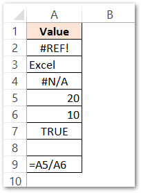
Use the following ISERROR Formula in cell B2 and copy it to other cells in column B.
=ISERROR(A2)
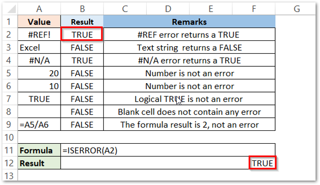
The Remarks column in the above image clearly explains the reason for the ISERROR function output.
Ex. 2 – Counting Total Number of Errors Using ISERROR with SUM Function
In this example, we will pass a range of cells to the ISERROR Function and then use the result to count the number of errors. Below is the required range of cells.
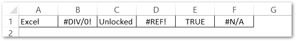
Enter the following formula in the target cell and then simply press Ctrl + Shift + Enter on your keyboard.
=SUM(--ISERROR(A1:F1))
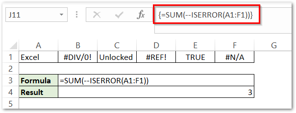
As a result, the formula returns the total number of errors to be 3.
Explanation – Let us see in steps how did the formula conclude this result.
- ISERROR function checked the error for the range A1:F1 and returned the result as an array {FALSE; TRUE; FALSE; TRUE; FALSE; TRUE}
- We applied the unary operator (–) to the array and converted the result to {0;1;0;1;0;1}. 0 for logical FALSE and 1 for logical TRUE.
- Finally, the SUM formula returned the sum of the array of elements 0+1+0+1+0+1=3.
When we press ctrl+shift+enter after typing the array formula, excel automatically adds curly brackets around the formula. You can also check the highlighted formula bar in the above example.
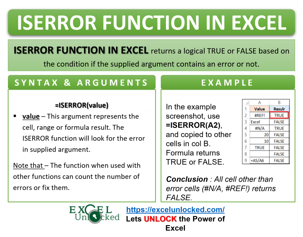
Ex. 3 – Cleaning Errors By Using IF function With ISERROR Function
While working with formulas in Excel, we might need to represent the results formally in a clean way. Instead of displaying the fussy error messages like #NUM!, #REF!, #DIV/0, we can give any other alternate text string.
Look at the below example. Here we have divided the values in column A with values in column B.
=A2/B2
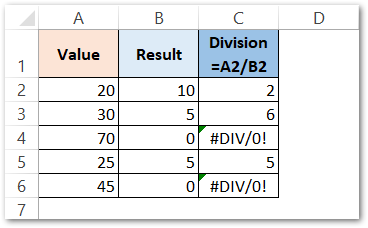
As a result, the formula performs division.
You will notice that the formula returned #DIV/0! error code in cells C4 and C6.
Use this formula to fix excel error messages.
=IF(ISERROR(A2/B2),"oops!",A2/B2)
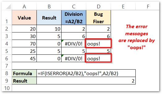
As a result, the formula returns the text string “oops!” instead of actual excel error message.
Explanation – The condition in the IF formula is ISERROR(A2/B2). If the division of A2 and B2 gives an error then the formula returns TRUE, otherwise, it returns FALSE (for no error). When the IF formula condition is TRUE, the function displays a text string “oops!”. If the condition is FALSE then the result will be A2/B2. The condition is TRUE for cells C4 and C6 (erroneous cells) thus the function returned a text string “oops!”.
This brings us to the end of the function blog!
Thank you for reading 😉
RELATED POSTS
-
ISERR Function in Excel – Checking If The Cell Contains An Error
-
ISNA Function in Excel – Checking for #N/A Errors
-
ISREF Function in Excel – Checking for Cell Reference
-
T Function in Excel – Usage with Examples
-
ISLOGICAL Function in Excel – Checking for Boolean TRUE/FALSE
-
8 Errors in Formula in Excel and How to Resolve
The Excel ISERROR function checks whether a value is an error. The function only returns TRUE upon finding an error and returns FALSE for all other values.
ISERROR, which literally means ‘Is error?’, tests all types of Excel errors. Making its entry into the Excel world in 2003, ISERROR comes from a group of IS functions that results in TRUE or FALSE. The syntax of the ISERROR function is just one value argument (like all the other members from the IS functions family). Let’s have a look.

Syntax
The syntax of the ISERROR function is as follows:
=ISERROR(value)
Arguments:
value – The value or expression that needs to be tested for errors.
Important Characteristics of ISERROR Function in Excel
- The ISERROR function deals with all formula errors in Excel, the function returns TRUE when it finds an error, otherwise, it returns FALSE.
- ISERROR is most commonly used with the IF function to find and handle errors.
- In Excel 2007 or higher, you can use the IFERROR function instead of using ISERROR with the IF function to handle errors.
Examples of ISERROR Function
Let’s have a look at the basic work of ISERROR before we go into expanding its functionality.
Example 1 – Simple ISERROR function
The ISERROR function in its plainest form would look something like this:

Here, column A is listed with all possible Excel errors. We are using the ISERROR function at its simplest to check column A for errors:
=ISERROR(A2)
The ISERROR function finds an error in «A2» and returns «TRUE». The same goes with cells «A3» to «A8» all of which contain different error types. ISERROR results in FALSE upon finding no errors in «A9» and «A10». This shows that the ISERROR function traps all types of formula errors.
Now that the ISERROR function has made its introduction, let’s see what else it can do.
Example 2 – ISERROR function with IF function
The IF function in Exel is the easiest way to get most functions to be more user-oriented. The IF function checks if a given condition is met or not and returns the value set for either case. Let’s say we are in favor of attaining these custom values and not TRUE/FALSE. Using the ISERROR and IF functions together will help us with that. Let’s refer to an example.
Here, we have a dataset from 10 types of T-shirts. The data we have regarding the T-shirts are the total sales for each design type and its unit price. Our objective is to calculate the units sold of each type (dividing sales by price).

The #DIV/0 errors have occurred due to some missing prices of products. These don’t give our worksheet a nice look. Let’s try to present these errors in a better way.

Using the following formula, we have swapped the #DIV/0 errors out with a custom value «Error!»:
=IF(ISERROR(B2/C2),"Error!",(B2/C2))
Starting with the «Basic half sleeve T-shirt» in cell B2, the ISERROR function checks «B2/C2» for errors. Since, in this case, no errors are found; ISERROR’s result is FALSE. For a FALSE result, the IF function is set to display the result of «B2/C2» (which is 2,418.90/21.99 = «110»).
Now, let’s analyze cell D6. Since the ‘Yoke neck T-shirt’ is out of stock so its price and total sales numbers are not available. Here, the ISERROR function checks «B6/C6» for an error and finds a #DIV/0 error (0/0 = #DIV/0), so ISERROR returns a TRUE. For a TRUE result, instead of showing the #DIV/0 error, the IF function is set to display the supplied value «Error!».
Example 3 – ISERROR function with the SUM function
We can use the SUM and ISERROR functions to count the total number of errors in a range of cells.
Let’s take a look at Example 1.

The formula used is:
{=SUM(--ISERROR(A2:A10))}
Note: This is an array formula and must be entered with Ctrl + Shift + Enter keys, except in Excel 365.
The ISERROR function applied to the range on its own will split into the supplied cell range and give the result of each cell individually like this:

Upon finding errors from «A2» to «A8» and no errors in «A9» and «A10», the result of the ISERROR function is TRUE, TRUE, TRUE, TRUE, TRUE, TRUE, TRUE, FALSE, FALSE. The double unary operator in the formula converts TRUE and FALSE into their respective numeric values as 1 and 0. The result now is 1, 1, 1, 1, 1, 1, 1, 0, 0. The SUM function takes ISERROR’s result, adds it up, and displays «7» as the final result.
ISERROR vs IFERROR
IFERROR is like having the ISERROR and IF functions combined in one to give us lesser work to do. Upon finding an error, the IFERROR function returns a custom value otherwise it returns the value of the expression itself.
Sounds like a winning situation. Let’s see if it is.

Here we have used the data from Example 2 but switched IF and ISERROR functions for the IFERROR function alone. Here’s the formula we used:
=IFERROR(B2/C2,"Error!")
How does it work?
The IFERROR function checks «B2/C2» for errors, it finds the expression error-free and returns the result of the expression as it is (which is «110»). Coming down to the #DIV/0 error in cell D6. Since B6/C6 results in a #DIV/0 error, so the IFERROR traps the error and returns a custom value «Error!» which it displays as the final result.
Now it looks like a winning situation too; we have attained exactly the same results as with the ISERROR and IF functions combined. Also, note how simple and easy to read this formula is in comparison to Example 2.
How to Choose Between ISERROR & IFERROR
Both functions cover all Excel kinds of formula errors.
The ISERROR function by itself will result in TRUE/FALSE and hence requires the IF function to return a more meaningful output.
The IFERROR function on the other hand returns a custom output when the supplied expression results in an error. It is simpler than using ISERROR and IF together.
Another point worth noting is – IFERROR function automatically assumes that you will always want the result of the expression if your expression doesn’t have any errors. ISERROR, on the other hand, gives you a boolean value (either TRUE or a FALSE), and when combined with the IF function, it allows you to have more control over the result in both outcomes.
ISERROR vs ISERR
Why has there been so much emphasis on ISERROR covering all Excel errors? There are some functions that by design deal with lesser errors.
Little brother of ISERROR, ISERR deals with all Excel errors except the #N/A error. ISERR function returns TRUE if any error (except the #N/A error) is detected and FALSE for #N/A errors and all other values.
This may seem like a shortfall but could be handy where #N/A errors don’t need to be accounted for by the function and need to stand out as missing information instead of other errors. Let’s look into this with an example.

We are trying to find the units sold of certain shirt types with this formula:
=IF(ISERR(VLOOKUP(F6,$A$2:$D$11,4,0)), "Error!", (VLOOKUP(F6,$A$2:$D$11,4,0)))
That seems like a lot to take in but that’s why we’re here.
In the first case, VLOOKUP’s job is to find the value mentioned in cell «F6» from the first column of the table «A2:D:11» (the «$» signs are to keep this table constant in the formula). The value to return is in the «4th» column. «0» in the formula means that an exact match must be found by VLOOKUP.
This formula finds «Longline T-shirt» in column A, picks up the corresponding value from column D which is a «76». Next, the ISERR function evaluates VLOOKUP’s result, which is not an error and so «76» is returned as the final outcome.
In the second instance, VLOOKUP was unable to find «Shortline T-shirt» in column A as it is not listed in our dataset. VLOOKUP returns the #N/A error. The result is passed to ISERR which does not handle #N/A errors and displays the #N/A error. This outcome is favorable in this case as using the ISERR function will account for other errors and deliver «Error!» and #N/A errors will show up to indicate that data is missing.
All things the same, this is what will happen if we replaced ISERR with ISERROR:

The ISERROR function traps all errors including the #N/A errors. This makes it hard to pinpoint that the error in the second instance is because «Shortline T-shirt» is missing from our set of data. In this instance, it’s more helpful to use the ISERR function.
How to Choose Between ISERROR & ISERR
The #N/A error usually comes up with lookup functions so, if the worksheet in question is not working with lookup functions, good chances are that the #N/A error won’t pop up to ruin the day. In that case, there isn’t a need for dealing with #N/A errors and the ISERR function would be a good pick. In case a #N/A error comes up, it can be handled by correcting the missing data (which is what #N/A errors indicate).
The ISERROR function heroes all Excel errors. It will trap and treat all errors, with the inclusion of the #N/A error, signaling the presence or absence of any errors in the data.
The results of ISERROR and ISERR are in TRUE/FALSE form and both may take help from the IF function to change TRUE/FALSE into more meaningful outputs.
That’ll be it for now. By now you may have gotten an idea on how to go about error dealing as annoying as they may be. Reminds us of a joke:
I hate spelling errors.
You mix up two letters and your whole post is urined.
We hope this didn’t ruin our whole post.
In complex spreadsheets it is very easy for error values to creep into a function or formula that you have used.
These can occur by accident such as simply deleting a tab or column that the function refers to. One moment, all is well on your spreadsheet, the next you see error values appearing. How did they get there?
It is important to understand why the errors can occur and the various types that you may see in a spreadsheet:
#VALUE! – This error occurs when you use the wrong data type as a parameter in a function e.g. you enter text into the parameter of a function when the parameter expects a numeric value or a cell reference.
=SUM («A1:A10») will produce this error because the function is expecting a valid cell reference, whereas the cell reference has been entered in quotes which designates it as a text string.
The formula should read =SUM (A1:A10)

Note that a green triangle appears in the top left of the cell, and an exclamation mark which if you hover your cursor over this will give you a pop-up menu. This will be discussed further in the article

#NAME? – this occurs if you spell a function name incorrectly or enter a function that does not exist. It can be very easy to make a typo when entering a function. In this example, SIM is a non-existent function.

The easiest way to get around this error is to use the handy drop down that appears when entering a function, so you will always get the name right.
#DIV/0 – if you have a number that is being divided by another number and the divisor is zero, then you will see this error. Note that the divisor could easily be to a cell reference on another sheet and because of imported data being used this could have a zero value when it had a number before

This error will also occur if the divisor refers to a blank cell.
You can use the IFERROR function to ensure that a zero value is returned for an error value in this case where a zero divisor has occurred. However, it could be dangerous to suppress other error types with this function, since they may need properly correcting!
#NULL! – This error comes about usually because you have specified a range without using a colon between the start and finish or you have ranges as parameters that do not intersect.

The formula should read =SUM (A1:A10)
The easy way to avoid this error is to use your cursor to select the range required instead of manually typing in the cell references
#REF! – this error comes about because you are refencing a cell or range location that no longer exists. It is usually because you have deleted a tab in the workbook, or a column in the spreadsheet which contained a cell that was referenced by your formula

The formula at cell A1 refers to the cell K14 on Sheet7. If column K on Sheet7 gets deleted, then the cell reference no longer exists and this error will appear.

#N/A! – This error is caused by using a function such as a lookup formula and searching for a value that does not exist.

In this example, the search criterion is a number, but it has quotes round it which designates it as text. Column B has numeric values not text, so the value cannot be found and return N/A
#NUM! – if your formula contains a numeric value which is not valid, then you will see this error
For example, using the square root function for the value of -1 will produce this error, since the square root of -1 does not exist

####### — when you see a row of hash signs displayed in a cell, it simply means that the value in the cell is too large for the column width
Either adjust the column width to show the full value or use alignment formatting to wrap the text or merge it into the next cell


Circular Errors
These come about, often inadvertently, because your formula refers to a cell which, possibly by a convoluted route, is taking the value from your current cell reference. Circular references can give incorrect results and should be removed as soon as possible
If you do try to enter a circular reference, you will get a warning message:

Whatever you do on this warning message, your circular formula will still be entered, but you will see a warning at the bottom left hand corner of the sheet. Also, the cell with the circular reference will be highlighted on each sheet in Excel 2019

You can use the ‘Formula Auditing’ group on the ‘Formulas’ tab of the ribbon to find all the circular references within the workbook. Click on the ‘Error Checking’ icon and then on ‘Circular References’ in the drop down, and you will see a list of circular references.

Linking Errors
You may be using a spreadsheet that has cells linked to values in another spreadsheet. The problem here is that if you have been emailed the spreadsheet but not the one that it links to, or someone has removed or changed the name of the linked spreadsheet, then this can cause problems
As soon as you load a spreadsheet with links in it you will see this warning message which gives you the option to update the link or not as the case may be.
Whichever option that you take, you will get a #REF! error if the linked file cannot be found.


If this is on a spreadsheet that you are not familiar with and do not have access to the linked file, you may wish to dispense with the links, since every time the file is opened you will get a message regarding updating of the links. This can be extremely irritating for users if they do not have the file
You can see all the links in a spreadsheet by using ‘Edit Links’ on the ‘Queries & Connections’ group of the ‘Data’ tab on the ribbon

You can use the ‘Break Link’ button to remove the link. However, this will still leave the error #REF! as a text string in the cell and it will not show as an actual error so cannot be tracked. You can use ‘Find and Replace’ (CTRL-F) to find this cell but the problem is that it no longer has the data in it.
You can do a Copy and Paste Special (values only) to leave only the number, but how do you find where the linked cells are? The ‘Edit Links’ pop up does not give this information
Linked cells always use square brackets ([ and]) to define the linked filename. Use ‘Find and Replace’ (CTRL-F) to search for a square bracket within the workbook, and this will lead you to where the linked cells are. You can then edit change the cell to a value instead of a linked formula
Tracking the errors
In all these errors, with the exception of the multiple hash signs, you will see an exclamation mark on a yellow background adjacent to the error cell.
Hover your cursor on this and a pop-up menu will appear where you can obtain more information on the error.

This will give you options to help you sort the error out, including ‘Ignore Error’ which is not recommended!
You can also change the Error Checking Options from this menu:

You can use the ‘Error Checking’ icon in the ‘Formula Auditing’ group in the ‘Data’ tab of the ribbon to check for errors.

This will allow you to step through the errors on a selected tab, giving information about the error, and showing the calculation steps.
Note that this only works on the selected tab, not the whole workbook.
You can also use ‘Trace Error’ on the Error Checking drop down. This will place arrows to indicate the cells that affect the error value

#excelerrors #excelvalidation #excelchecking #excel #spreadsheet
If you find this article is helpful and you want to help others too, just share it in any social media (such as Facebook, LinkedIn).
Got it Pass Team is happy to work with Richard in presenting this article.
About Richard Shepherd-
Richard is an expert in MS Excel and Access with extensive experience of developing MI reporting systems, databases and dashboards using VBA or RAD for major companies such as Santander, Nationwide Building Society and Zurich Insurance. He is also the author of Access 2010 VBA Macro Programming and Excel VBA Macro Programming. He was graduated in University of the Thames Valley, United Kingdom.
Note: Some of the links in this page contain affiliate links. I will earn a small commission for any purchases you make, though there is no extra cost to you.
The products or services I recommend only I use them myself or after my investigation and truly believe they are useful to you. Don’t forget there are many other options out there – these are simply my preferred choices.