
Welcome to our Excel add-ins section. You can find here commercial and free charting and productivity tools for Microsoft Excel.
Excel Chart Add-ins
We love Excel data visualization tools and dashboards! We strongly recommend our chart add-in to build custom charts and graphs and improve your presentation.
Ultimate Dashboard Tools (Chart Add-in for Windows and Mac)
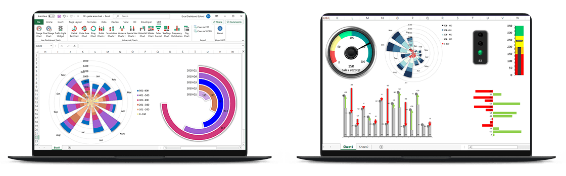
UDT is our flagship! The add-in enables you to create stunning charts and live widgets for Windows and Mac.
Category: Commercial
Learn more about the tool.
This page is dedicated to extending Excel application functionality.
DataFX Function Library
The add-in contains almost 200 high-performance user-defined functions. Create easy-to-read formulas and speed up your work! We are investing even more developer hours and energy to improve the add-in continuously. The add-in uses the Intellisense Excel-DNA framework that provides native tooltips for user-defined functions. If you want to look at the categories, you can use the function browser.
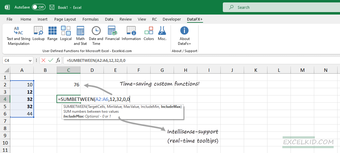
The current version of the add-in core functions, for example, DXLOOKUP, ensures XLOOKUP compatibility for all Microsoft Excel versions. Take a closer look at how useful the tool is. We update the library weekly and will implement even more functions in the next few months.
Category: FREE

If you want to learn more about the integrated functions, don’t hesitate to look at the PDF files containing useful examples.
Learn more on how to install an Excel add-in!
DataXL Productivity Suite
DataXL dramatically increases your productivity. You can use various time-saving tools, like data cleansing tools.
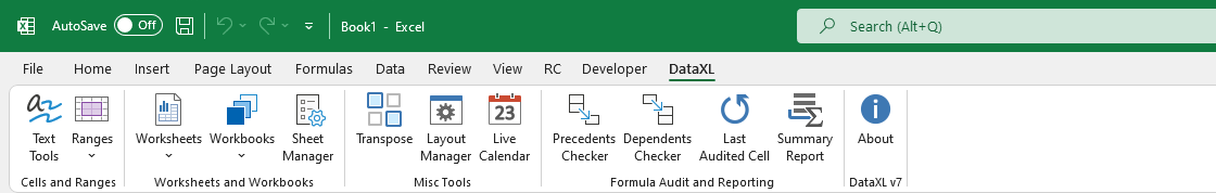
List of the most important features:
- Text manipulation tools
- Range functions
- Workbook and Worksheet functions
- Sheet manager
- Live calendar
- Layout manager
- Precedents and Dependents checker
Category: FREE
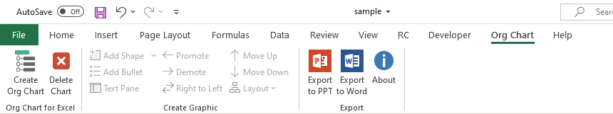
Org Chart Add-in
Organizational Chart Builder creates great org charts using raw data. If you are in HR, it is a must-have plugin! Place your raw data and create a structure with a single click.
Category: FREE
Download the add-in
Following versions of Excel are supported by ChartExpo

Excel 2013 SP1 or later on Windows

Excel 2016 or later on Mac

Excel 365 on Windows & Mac
The ChartExpo Excel add-in simplifies data visualization and offers a wide range of custom Excel charts for you to use.
Finally, charting is fun and accessible to everyone.
With an ever-growing library of advanced Excel charts, there is an option for all your charting needs.
No matter what Excel chart types you need, ChartExpo has it.
If we don’t have what you need, we’ll create it for you! It takes just three clicks to start making graphs in Excel with ChartExpo.
There’s no coding, scripts or complicated settings to navigate.
It’s an easy-to-use charting tool that anyone can benefit from.
Start finding meaning behind your numbers.

Build Advanced Excel Charts Simply
As the data grows, the need for advanced Excel charts rises. Traditional graphs in Excel don’t always offer the depth of visualization that you need for more sophisticated data sets.
With ChartExpo’s Excel add-in, the doors open up to a library of advanced Excel charts that are exceptionally easy to use.
Choose from new Excel chart types, like Sankey, Pareto, Likert, dayparting, polar, comparison, survey charts and so many more.
Excel is a familiar and intuitive tool used by millions, but it does have some deficiencies, especially when it comes to charting and visual data storytelling.
When the need arises for advanced Excel charts to accurately convey your ideas and results, these shortcomings of Excel will get in your way and slow down your visual analysis.
ChartExpo doesn’t just offer new advanced Excel charts to capture your data visually. The real value is the simple ways that this charting tool transforms even the most complex spreadsheet into a refined, digestible visualization.
Simplify Your Analysis
Your data is already complex enough. Visualizations need to improve your understanding of your spreadsheets, not to detract from it.
ChartExpo’s advanced charting options can demystify convoluted spreadsheets by simplifying the information through visuals.
An advanced chart shouldn’t be overwhelming or difficult to understand. The most effective visual analysis occurs when you take complicated information and depict it in the simplest format.
Simple is not basic and rudimentary. When you solve a complex problem with a simple solution, simple becomes revolutionary. This is the case when you tell the entire story of a spreadsheet with a single chart.
Thus, the most effective data stories are the ones that present the information in the simplest and most direct manner. This allows the audience to arrive at the correct conclusions instantaneously.
Start simplifying your visual analysis today.
Fast Discovery Creates Swift Action
The instant insights you receive from ChartExpo’s advanced Excel visualizations save you both time and money. After all, the faster you can reach the right data conclusions, the better the value.
ChartExpo’s easy-to-use, advanced charts for Excel make experiencing those monumental “Aha!” moments a regular occurrence.
An “Aha!” moment is when you finally “see” your data and reach the conclusions you’ve been trying to find in your spreadsheets.
With the right Excel charts, these sudden bursts of inspiration rise to the surface. You don’t have to exert tons of effort to uncover insights. They are right in front of your eyes the moment you visualize them!
Fast discovery leads to swift action. The faster you act on data, the more weight those actions carry. This is because your data may have a short shelf-life. So, you don’t want to waste too much time analyzing the information and choosing how to react.
Instead, you want to quickly discover the most important details hidden in your data and respond as promptly as possible.
Mitigate Risks, Capitalize on Opportunities
Trends, shifts, outliers and other patterns in your data are either positive or negative. Negative changes present potential risks, while positive ones represent emerging opportunities for you to seize.
This is why it’s imperative that you use advanced Excel charts to respond swiftly to your data and insights.
Think of a risk change as a leaky pipe. The longer you let the leak exist without fixing it, the more damage it causes. Water damage eats at surrounding wood and other materials, creates mold, etc. However, if you detect the problem as soon as it starts, you can fix it with no damage.
Time is also an important element to positive data trends and shifts. When you identify this type of change in your custom Excel charts, you want to be one of the first to act.
Many of these trends are like fads; they come and they go. You want to get in on the ground floor and be the first to capitalize. Otherwise, you’ll be rushing to catch up with the trend, instead of already riding the wave.
Speed is especially critical in businesses. You may be interacting with lots of the same data as your competitors. You gain a significant edge over these other entities if you can leverage the insights hidden within this sea of data faster than your competitors,
By empowering your spreadsheets with ChartExpo’s excel add-in for data analysis; you can stop leaks and capitalize on top trends faster and more efficiently.
That’s a competitive advantage you don’t want to miss!
More Charting Options, More Advantage
The competitive advantage you receive from acting on insights faster is key to any data user’s success. Another element of a winning visual analysis strategy is having a deep bench of charting options available to use.
ChartExpo’s interface makes it quick and easy to perform visual analysis from multiple angles. Each custom Excel chart type you use will showcase your data in a new light and reveal fresh insights that are both valuable and actionable.
Since ChartExpo allows you to visualize your data with new advanced Excel charts in as few as 3 clicks, it’s incredibly easy to cycle through multiple chart types and find the best ways to convey your findings and insights.
Every time you view your data with a new visualization, your understanding expands and you gain further details that flush out your data story.
Including multiple visualizations in your reports empowers your visual data storytelling by showcasing the information from several angles.
Plus, ChartExpo graphs in Excel are interactive, making it easier for you and audiences to engage with your data and uncover new insights.
More Excel chart types mean more value.

Custom Excel Charts for any Data and any User
Your data needs are unique, meaning you want to go beyond traditional Excel chart types. Thanks to ChartExpo’s custom Excel charts, you can customize any element of your graphs. Each change is simple to make and helps you deliver completely customized charts.
Custom charts help you communicate data findings to audiences, leading to more effective collaboration that helps you uncover even more exciting trends, patterns and insights.
Start making your own graphs in Excel that will wow your audiences.
Every Excel user is different and so is their data. Custom Excel charts help you match the right visualization to your data sets, while also personalizing your charts in ways you see fit.
Through ChartExpo’s simple visualization tool, you can customize any element in your charts, even down to the colors, fonts, axes and more.
These customization options ensure that you always present your data in the best ways possible, thereby empowering your visual data storytelling
Chart Type
To reiterate, data is unique and capturing its value and insights requires you to match your numbers with the proper graphs in Excel.
Unfortunately, this isn’t always possible with the stock Excel charting options. The traditional visualizations available with the Excel software handcuff you into using only a handful of basic charts.
The ChartExpo tool vastly improves these lackluster charting options by providing you with a library of advanced Excel chart types for you to customize your visualizations and strengthen your data storytelling.
With so many Excel chart types to choose from, there’s an option for all of your data objectives. If you need to portray the results of a survey, use the CSAT Score Survey Chart or Likert Chart options. Alternatively, if you want to depict different stages in a complex process, the Sankey Diagram is an excellent choice.
You can even leverage the word cloud or text relationship charts to express new keyword opportunities. No matter your reasoning for using Excel, ChartExpo has you covered with its ever-growing selection of visualizations.
If you can’t find the right graphs in Excel with ChartExpo, we’ll build it for you. The engineers behind ChartExpo are always listening to our users and finding new ways to deliver the best custom Excel charts.
ChartExpo’s user-friendly design makes it easy to find the best visualization for your data needs. Excel chart type categories help you find the right graph for every project.
Once you find the right category, it’s a simple matter of selecting each Excel chart type until you find the one that best suits your data and objectives.
Title
Every good story needs a great title; visual data stories are no exception. A proper chart title showcases what information is portrayed and establishes the audience’s expectations as to what conclusions they may draw from the graph.
Thus, your chart title has a direct purpose and definite value. It’s not an area of advanced Excel charting that you want to overlook.
The best chart titles manage to entirely explain what’s being shown in the chart using the fewest words. Concise titles are the most effective because they are easier to understand, look more professional and save time. The fewer words you use, the less chance of confusing your audiences!
Unfortunately, making short titles isn’t always easy, especially when using multiple variables to accurately describe your chart.
You may find yourself making minor changes to your title repeatedly to find the perfect one. Luckily, ChartExpo makes it easy to create new titles or update existing ones.
In fact, you can edit any component of your chart in a few simple steps. Customizing or updating your charts is never a hassle!
Colors, Fonts and More
Your chart title explains what data you’re depicting. It’s an essential part of compelling visual data storytelling. Smaller components, like the colors, fonts and other details you choose, also matter.
Not only do these elements make your graphs in Excel more engaging, but they can also help you convey your results more effectively.
For instance, color is a valuable tool to keep different data categories separated, like in a stacked bar chart.
You can even use colors to depict what’s actually being shown. If you’re visualizing weather data, blue can represent cooler temperatures, while red depicts warmer ones.
On the other hand, fonts need to be legible and professional. You also don’t want to choose a font that distracts from the chart itself. Many businesses elect to use fonts that match their branding and other correspondences.
Keep your audience in mind whenever you choose fonts, colors or other small details. You want to try and view your data as an unbiased party and answer critical questions, such as, “Do the colors/fonts add to the visual analysis or take away from it?”
Similar to editing your title, ChartExpo also makes it fast and simple to edit your visualization’s fonts, colors and other minor (yet still important) components.
Axes
Chart axes represent your variables and allow you to compare distinctly different items or categories from your spreadsheet.
A typical chart will have two axes, enabling you to chart two items in your spreadsheet, a metric and a dimension.
That said, you may run into times when you need advanced Excel charts with more axes to depict your data accurately. As you add axes, you can compare and contrast more items in one chart.
ChartExpo has several multi-axis Excel chart types to choose from, making it exceptionally easy to add or remove variables and axes.
These advanced Excel charts can even compare data with vastly different ranges, allowing you to compare data values that are extremely different from one another. This would be difficult to achieve with traditional Excel charts.
ChartExpo also includes Excel chart types with unique axes. For example, the radar chart features a circular axis perfect for tracking changes over time
Be careful of adding too many axes and variables. This will overload your Excel charts and make it challenging to extract insight and act on the information shown.
Deliver a Complete Presentation
The impact of all of these small components to your visual data storytelling may seem small. However, getting each of these elements correct vastly improves your ability to convey visual data and engage audiences.
ChartExpo makes it effortless to edit every component of your custom Excel charts. This makes it easy to make even small changes without starting over or waiting for a new chart to load each time.
It also means that finding the correct mix of chart type, title, colors, fonts and more is much easier. You can keep making adjustments until you find the right combination!
These complete, custom Excel charts will empower your reports and help you deliver outstanding presentations with beautiful, engaging charts. Audiences won’t want to put your data down.
An outstanding data presentation does a lot for your internal communication. Plus, it helps build organizational trust and understanding of what the data shows and how to use it.
Once you create your first custom Excel charts with ChartExpo, you’ll see the impact it has on your presentations.

The Easiest Way to Make Graphs in Excel
You spend enough time collecting data, creating spreadsheets and organizing your columns and rows to extract insights.
Creating advanced Excel charts is the best way to discover and communicate these insights. Don’t let it become another time-consuming step in the process.
With ChartExpo’s intuitive, easy-to-use Excel add-in for data analysis, you can make beautiful, insightful graphs in Excel in just 3 clicks.
The time you save through effortless advanced Excel chart creation is time you can spend on other projects and deeper data analysis.
Building advanced charts within the Excel interface comes with several obstacles. It’s common to find yourself cycling through multiple tabs and spreadsheets just to create one visualization.
Not only does this slow down your visual analysis and keep you from those all-important insights, but it also heightens the risk for errors to occur.
ChartExpo allows you to overcome these obstacles. The most significant weaknesses of Excel charting become your best sources of strength thanks to the easy-to-use charting interface.
Universal Charting
There shouldn’t be a skill gap to creating outstanding visualizations. Yet, producing advanced Excel charts without ChartExpo’s easy-to-use system requires a deep understanding of how the spreadsheet tool works.
This can make it challenging for novice Excel users to create effective, advanced charts in Excel. There are so many settings, shortcuts, inputs and other components that you have to learn to make charts and graphs in Excel.
ChartExpo eliminates this hassle with a highly intuitive charting interface. This means anyone can conduct deep visual analysis, no matter how complex the data is.
All it takes is three clicks. First, select which part(s) of your spreadsheet you want to chart. Second, click the chart type you want to use. Finally, you tap the “Create Chart” button.
That’s all it takes. There are no fancy scripts, complex coding or extensive options and settings to navigate.
Making edits to your custom Excel charts is also easy with ChartExpo. And, every adjustment to your chart updates the visualization instantly, so you can immediately see the difference in every change you make.
This feature also enables you to cycle through ChartExpo’s massive, growing library of chart and graph types. You can see how your data looks across these various visualization options and discover the best ways to present the information.
You shouldn’t have to be an Excel wizard to transform your spreadsheets into engaging data stories. With ChartExpo, you don’t have to be.
Code-Free Environment Means no Stress
ChartExpo’s codeless environment does a lot to even the gap between advanced Excel users and novice ones. Even if you’re already a master at Excel, there’s still significant value to gain from a codeless, script-free tool.
It’s critical to keep in mind that this is an Excel add-in for data analysis. It doesn’t aim to replace Excel or your spreadsheets.
The goal of ChartExpo is to supercharge your visual data storytelling through Excel by providing a library of easy-to-use charts for fast, but detailed, analysis.
By removing the coding requirement, ChartExpo eliminates potential obstacles and makes charting and data storytelling more accessible than ever.
Remember, you might interact with your data and create Excel charts often, but other parties don’t have the same level of familiarity. ChartExpo’s easy-to-use interface means that anyone on your team can interact, alter and share charts, or create ones of their own.
The more parties involved in visual analysis, the more potential insight your organization can gain.
Remove the tiresome coding and make charting an accessible, engaging activity.
Faster Charting Saves Time and Money
Your time is valuable, no matter what types of data you’re dealing with or what your objectives and goals are.
Chances are, you’re juggling multiple projects and responsibilities at the same time. When charting and visual analysis takes too long, it eats away time from these other tasks and adds unnecessary stress and pressure to your daily to-do list.
The 3-click process means you can make sophisticated visualizations in just minutes. This leaves you with more time to focus on the visual analysis itself to capture even greater insights.
There’s no more fussing across multiple spreadsheets and tabs in the pursuit of making a simple chart. ChartExpo simplifies the arduous process to save you all the headaches from traditional Excel charting.
The other significant source of wasted time in Excel charting is how long it can take for the application to load and display your chart. An advanced Excel chart can take up to 15 minutes to process and appear.
When you make adjustments to your spreadsheet or chart, you may end up waiting even longer for your visualization to update.
Meanwhile, creating or editing Excel charts with ChartExpo happens instantly. There’s no disruption to your visual analysis! As soon as you click Create Chart, your visualization appears. There’s no waiting!
By saving time with smoother, more efficient charting, you also save money. That’s something that every Excel user can get behind.
Optimize Your Workload
Thanks to ChartExpo saving you substantial time in the visualization process, you can greatly optimize your workload and finish more high-priority tasks and projects in less time.
The speed at which you can glean insights and discover new trends, shifts and other patterns with ChartExpo enables you to analyze more of your total data.
When you’re working with massive spreadsheets and mountains of data, trying to analyze all of it feels like an impossible task.
By alleviating the time pressures of some of the more tedious steps in the analysis process, such as charting, you have more time to explore other areas of your data.
Applying the proper chart to your data allows you to physically see how data points relate to one another. Noteworthy patterns and other events rise to the surface.
It’s these now-visible insights that expand your actionable intelligence and provide you with a deeper understanding of the data. ChartExpo’s data visualization software puts insights in clear view.
The faster you detect and analyze insights, the sooner you can react appropriately. In a business setting, this can mean gaining a significant competitive edge through continuous improvements to your key metrics.
Start optimizing your visual analysis with ChartExpo and see the benefits for yourself.

Explore New Excel Chart Types
With ChartExpo’s extensive library of Excel chart types, you have all new graphs and visualizations to explore.
These advanced Excel charts give you fresh angles to view your data. Each new perspective offers the chance to see new, previously undiscovered insights. You’ll see the unseen and gain actionable intelligence that others don’t have access to with their existing Excel chart types.
Begin exploring and communicating your data in new ways today.
ChartExpo opens the door to many new Excel chart types ready to solve your most complicated data sets.
Within the standard Excel program, you only have a handful of chart types to choose from. This limits how much freedom you have when designing custom Excel charts.
Even with advanced tools and techniques, it would be impossible to create some of the advanced Excel charts included with ChartExpo.
Excel Chart Types to Choose From
ChartExpo has no shortage of Excel chart types, giving you more freedom and capability in the visual analysis stage.
Many of the options included in the ChartExpo library have very specialized purposes. If you have very niche data needs, explore the advanced Excel charts included with ChartExpo. You may just find the perfect visualization!
Here’s a complete rundown of the Excel chart types available with ChartExpo:
| Sankey Chart | Likert Scale Chart | Pareto Bar Chart | Pareto Column Chart | CSAT Score Survey Chart |
| Radar Chart | Comparison Bar Chart | Gauge Chart | Chord Diagram | Sunburst Chart |
| Funnel Chart | World Map Chart | Column Chart | Grouped Bar Chart | Grouped Column Chart |
| Sentiment Trend Chart | Tree Map Sentiment Chart | Sentiment Matrix Chart | SM Comparison Chart | Sentiment Sparkline Chart |
| Comparison Sentiment Chart | Double Bar Graph | CSAT Score Chart (NPS Chart) | Customer Satisfaction Chart | Credit Score Chart |
| Rating Chart | Area Chart | Stacked Area Chart | Bar Chart | Stacked Bar Chart |
| Stacked Column Chart | Line Chart | Multi Series Line Chart | Crosstab Chart | Pie Chart |
| Donut Chart | Tree Map | USA Map Chart | Word Cloud Chart | Partition Chart |
| Area Line Chart | Sequence Chart | Sparkline Chart | Co-occurrence Chart | Tornado Chart |
| Dual Axis Grouped Bar Chart | Dual Axis Grouped Column Chart | Multi Series Sparkline Chart | Slope Chart | Dual Axis Radar Chart |
| Matrix Chart | 24 Hour Chart | Bid Chart | Tag Cloud Chart | Progress Chart |
| Performance Bar Chart | Dual Axis Line Chart | Double Axis Line and Bar Chart | Multi Axis Line Chart | Radial Chart |
| Quality Score Chart | Scatter Plot | Text Relationship Chart | Components Trend Chart | Control Chart |
| Context Diagram | Dot Plot | Grouped Dot Plot | Box and Whisker Column Chart | Box and Whisker Bar Chart |
| Overlapping Bar Chart | Dot Plot (ORA) |
Since the ChartExpo library is constantly growing, this list is always changing and increasing. Moreover, many of these Excel chart types have multiple variations, meaning this list is longer than it appears!
With so many Excel chart types to choose from, there is sure to be a specialized visualization for your various visual analysis projects, whether you’re looking at financial data, marketing metrics or any other information.
An Ever-Growing Library
Using a library of advanced Excel charts means you should find specialty visualizations for all of your needs, but what happens if you still can’t find what you’re looking for?
ChartExpo’s goal is to continue to deliver innovative visualizations that handle the current data needs of our users. Since data is always growing and evolving, our visualizations need to do the same!
If you have very specific or niche charting needs that aren’t covered by our list, we urge you to get in contact with us!
Depending on the situation, we may be able to work with you to create a visualization that solves your data challenges.
By solving our users’ needs and staying up-to-date on the latest data challenges facing the world, ChartExpo’s library of visualization options continues to grow and grow.
Change Chart Types to Discover New Insights
When you combine the expansive lexicon of charting options with the instant visualization power of ChartExpo, you have a tool capable of steadily generating insights.
These discoveries will improve your understanding of complex data and fuel better decisions regarding what to do with the latest figures.
Every new chart you use to visualize your data provides a new perspective and the opportunity to capture previously-unseen insights. The easy-to-use ChartExpo system allows you to simultaneously view your data from multiple angles.
You don’t have to wait for your chart to load each time you select a new type! This massive time-saver allows you to get more out of your data and your Excel charting options.
You can view the same data using multiple charts simultaneously, giving you the best view of your data and potential insights.
While most Excel users are drowning in data and starving for insight, you’ll be swiftly creating visualizations that yield deeper intelligence.
That’s the advantage of using ChartExpo!
Prevent Analysis Fatigue
When you only have traditional Excel charts to work with, you may not always have the perfect visualization to depict your data.
This puts you at a disadvantage for two reasons. First, it limits your ability to connect your data to the best chart, which means you may miss valuable insights.
The second problem is efficiency. Trying to fit your data into a chart that doesn’t exactly capture the information correctly is like trying to fit a round peg through a square hole. It’s going to take more time and energy to make it fit.
This tedium makes you very susceptible to analysis fatigue. Analysis fatigue manifests when you exert so much time and energy on a single analysis that it creates a paralyzing effect.
It’s essentially the result of having too much data that it becomes overwhelming, especially when you’re working with clunky, time-consuming charts. You put in an abundance of effort and receive very little value or intelligence in return.
ChartExpo’s hassle-free charting environment remedies analysis fatigue by speeding up and improving the visualization process. With more Excel chart types, you can go from raw data to insight in far fewer steps.
This saves time and headaches to ensure you’re always on top of your data, instead of struggling to catch up to it!

Simple Excel Add-ins For Data Analysis
There are many Excel add-ins for data analysis available to users. However, not all of these tools are valuable.
ChartExpo provides value in three fundamental ways:
- ChartExpo’s Excel add-in increases the number of available Excel chart types ten-fold.
- You can create advanced Excel charts with a simple 3 clicks.
- Every advanced Excel chart is entirely customizable, opening the door to limitless opportunities.
As an Excel add-in, it integrates into your existing spreadsheet platform. There’s no complicated software to navigate, just simple custom Excel charts ready to use.
Not Another New Tool to Learn
There are plenty of third-party tools and software available to data users. Yet, all of these solutions have one problem in common: familiarity.
See, we like tools that we’re used to. We also despise change. So, when adding a new solution to the arsenal, you want to ensure it meshes with your existing tools and strategies.
That’s why ChartExpo is an Excel add-in for data analysis, instead of a stand-alone tool. It integrates directly into the Excel environment, meaning you don’t have to master an entirely new piece of software.
Once you’ve downloaded the tool, you simply click “My Apps” from the top Excel menu bar and select ChartExpo.
Then, you’re just three clicks away from a beautiful visualization. Your first click selects the relevant data, the second chooses the chart type and the third finalizes and creates the chart.
The ChartExpo tool opens right in the Excel interface, so you don’t even have to switch tabs or copy-paste and details from one to the next.
This is just another way that ChartExpo simplifies the visual analysis process and allows you to be more efficient in your visual data storytelling.
Integrates Easily Into Excel
The process to integrate ChartExpo into the Excel interface is exceptionally easy.
Once you’ve created your account and downloaded the ChartExpo Excel add-in for data analysis, you should see it appear under the “My Apps” menu. If you can’t find this option, look under the “Insert” tab at the very top of your page.
After you open the ChartExpo tool, it’s a simple three-step process to begin creating new graphs in Excel.
- Select the data from your spreadsheet that you want to include as each axis variable. Depending on your chart type, you may have to enter multiple data columns representing these different metrics or dimensions.
- With your data selected, you now want to choose your chart type. ChartExpo divides visualizations into different categories to help you find suitable options for the job. Don’t forget, you can test how your data looks using multiple Excel chart types.
- After finding the perfect chart, all that’s left to do is hit the “Create Chart” button. The graph will appear alongside your spreadsheet data, allowing you to easily refer back to your data table as you conduct your visual analysis.
If you want to make any changes to your chart, like editing the title, colors or other small details, you can select individual components to modify.
Code-Free Charting
To make the learning curve for ChartExpo even easier, this Excel add-in for data analysis is designed to be entirely codeless. There are no scripts or languages to learn, just an intuitive interface.
The codeless Excel add-in holds many advantages. When you don’t have to worry about coding each chart, you can create visualizations much more efficiently.
Zero coding or scripting also means more people can engage in the visual analysis process.
While you may be familiar with all of the hidden features of Excel, not everyone in your organization has the same level of proficiency. ChartExpo closes the skill gap in creating advanced Excel charts and allows more parties to get involved in the visualization process.
This enhances your team’s visual analysis efforts by introducing more individuals to the world of charting. More people mean more hands on deck for discovering insights and tapping into your data intelligence.
You shouldn’t have to be an Excel pro to make advanced charts and graphs. With ChartExpo, anyone can start designing custom Excel charts today!
Experienced Excel users may argue that, without scripts and codes, they don’t have the freedom to make their own custom charts.
However, with ChartExpo’s colossal library of visualizations, you don’t need to make your own charts. Every Excel chart type you could want is already included!
Get More Value from Excel
ChartExpo for Excel costs $10 a month per user. You may be wondering why pay for an Excel add-in when Excel itself is free?
To answer this question, let’s recap how ChartExpo adds value to Excel users and visual data storytellers.
- ChartExpo saves you time in the chart creation process. When you save time, you also save money!
- Faster charting also allows you to promptly detect and resolve any risks or opportunities hidden in your data.
- With new Excel chart types, you’ll always have the perfect visualization for your data, regardless of the subject or complexity.
- More charting options increase the number of angles to view your data from, enabling you to discover deeper insights.
- The easy-to-use charting system makes visual analysis more accessible. You can start encouraging your entire team to create custom Excel charts!
- This intuitive Excel add-in for data analysis will also reduce stress and headaches caused by traditional charting.
- The advanced Excel charts will empower your reports and help you convey complex data to other audiences.
The list of valuable advantages provided by ChartExpo goes on and on. The bottom line is ChartExpo adds tremendous worth to your visual analysis that quickly makes up for this $10 per month cost.
You’ll be extracting so much more insight and value from your data; you won’t even notice this small monthly expense!
PineBI
The Ultimate Excel Charting Add-in

What is PineBI?
PineBI is a charting add-in for Microsoft Excel.
It’s a simple .xlam file — no installation is required (If you can open an Excel workbook, you can use Pine BI)

It allows you to insert advanced Chart Templates with just a click of a button.
The chart editor makes editing charts much easier
Other miscellaneous tools make building fancy reporting dashboards extremely simple.
PineBI does not need to be installed to edit charts created by PineBI. Once the charts are created, anyone can edit them.

Insert Chart Templates
Insert pre-built chart templates with just a mouse-click.
40 pre-set templates
All Pine BI created charts can be edited without PineBI Add-in.
Create Charts from Existing Data
Create beautifully formatted charts using your existing data ranges, Tables, or Pivot Tables.
Data ranges can even be located on different worksheets.
Charts come with numerous color and style variations.


Chart Editor
Simplified Chart Editor makes it easy to quickly apply basic formatting adjustments to your charts.
Excel doesn’t have an option to edit multiple charts at once. However, Pine BI makes it easy to quickly edit multiple charts at one time.
Also quickly split charts, replicate chart format, and much more!
Join the Satisfied Professionals Who Use Pine BI
«I’ve been using Pinexl dashboards for a few months and love them and the detail they display!»
Steve Sunder
President Sunder Vision Solutions

What’s Included
Actual Vs. Target Charts
Simple Bullet
Full Overlap
Partial Overlap
Thermometer
Column with Markers
Dynamic Color
Line / Area Threshold
Waterfall Charts
2 Versions
Horizontal / Vertical
Cards
Variance Charts
Column / Bar
Pin / Lollipop
Advanced (2 versions)
Gauges
Donut Gauge Chart
Speedometer (3 versions)
Heap Maps
Sequential
Diverging
Navigation Menu
Project Management Charts
Gantt with Progress
Milestone
RAG
Forecast Charts
Simple Forecast
Forecast with Confidence Interval
Other Charts
Min / Max
Income / Expense
Bullet
Tornado

Forecast Chart including Confidence Interval

Gauge Chart

Waterfall Chart

Tornado Chart

Variance Chart 1

Variance Chart 2

RAG Chart

Min / Max Chart

Milestone Chart

Gantt Chart

Income / Expenses Chart

Heat Map

Donut Chart

Card Chart

Bullet Chart

Actual vs. Target — Threshold Line Chart

Actual vs. Target Thermometer Chart

Actual vs. Target — Threshold Area Chart

Actual vs. Target — Overlap Chart

Actual vs. Target Marker Chart

Actual vs. Target DX Chart

Actual vs. Target Bullet Chart
Purchase Pine BI

FAQ and Other Information
What is your refund policy?
We have a 30-day, no-questions-asked, 100% money-back guarantee. If you’re unsatisfied for any reason, let us know and we will refund your order!
How do I edit or share charts created with Pine BI?
Pine BI is built on entirely native Excel features. Therefore you can edit all charts just like regular Excel charts.
Users without Pine BI will still be able to see and edit the charts you’ve created.
The charts are easily copied to PowerPoint or Word.
Will Pine BI work on my system?
Pine BI was designed to work on all Microsoft Windows systems (7,8,10, etc. and 32-bit or 64-bit). It will also work on all versions of Microsoft Office (2007 to present), including 64-bit Microsoft Office.
Pine BI also works on some Mac setups running Windows OS. However, it will not work on any versions of Excel for Macs (we expect a Mac version to be released in the coming months).
Note: The following charts will not work properly in Excel 2007 and 2010.
- Advanced Variance Charts V1
- Advanced Variance Chart V2
- Waterfall Charts
- Tornado Chart
Can I use PineBI on my work computer?
Pine BI is an Excel add-in (.xlam) file. No installation is required. No admin privileges are required. It should work on all computers regardless of IT restrictions.
If you can open an Excel workbook, you can use Pine BI
How do I download / install the add-in after purchasing?
After successful payment, you’ll receive an email with a license number and download link.
The add-in installs like any other normal .xlam add-in. There are no .EXE or .DLL files.
Detailed instructions will be provided after purchase.
How does the license work?
One license entitles you to use Pine BI on one computer at a time.
You can de-activate Pine BI on one computer and then active it on another computer as many times as you want. However, Pine BI can only be activated on one computer at one time.
Will my company pay for Pine BI?
Your company may have an allowance that will reimburse you for productivity tools like Pine BI. This is the case for some of our users. Ask your boss, HR, or IT!
How will I know if a newer version is available?
All new versions of the add-in will be sent to you via email.
Requirements
Publisher: Pinexl Ltd.
Supported OS: Windows 7 SP1 or higher*, Windows 8, Windows 10. Both 32 and 64 bit.
Supported Excel Version: Excel 2007 or newer**. Both 32 and 64 bit.
*If you are using Windows 7, make sure you have Service Pack 1 installed (you probably do). Pine BI cannot be activated otherwise.
**Waterfall charts, some Actual vs. Target charts and some other charts work best in Excel 2013 or newer.
Join the Satisfied Professionals Who Use Pine BI
«Amazing design and value! Waiting for the next products!»
Alexander Y.
Pinexl + Automate Excel
Pinexl specializes in Premium Microsoft Excel Tools for small and big businesses, like Excel Dashboard Templates and Add-Ins. All products are designed to be as modern, easy and as intuitive as possible to use, but at the same time to offer powerful insight into the data allowing for quick data driven business decisions.
Pinexl’s experience in multinational corporations is reflected in their products. With a minimalist and beautiful approach to visualizations, their products offer a professional and high-level way of showcasing and analyzing performance data, managing projects and making the daily work easier.
AutomateExcel.com is a proud affiliate of Pinexl’s Pine BI!
You’ll agree when we say Excel is a powerful tool for visualizing data.
And this is because it comes with a familiar user interface (UI). In other words, it has been there for decades. Besides, it has proven time and again to be amazingly reliable in storing and visualizing data.


Some of the best charts in Excel for data storytelling include Column, Bar Chart, Line, Area, Pie, Donut, and Combo charts, among others.
But, Excel produces pretty basic charts that require a lot of tweaking to be appealing or communicate insights fast. Besides, this spreadsheet tool lacks advanced charts that you may need to create compelling data stories.
Well, there’s a tool that supercharges your favorite spreadsheet tool. Yes, you read that right. This tool enhances Excel to generate insightful, visually appealing, and most importantly, easy to interpret charts.
This blog will walk you through how you can supercharge your Excel to create visually appealing and insightful charts. You’ll also get to learn about the top 5 best charts in Excel produced by our mysterious tool.
In this blog you will learn:
- Top 5 Best Charts in Excel Spreadsheet You Need to Try
- 5 Advanced Excel Charts You Can Create Using ChartExpo
- How to Create a Comparison Bar Chart?
- How to Create a Slope Chart in Excel using ChartExpo Add-in?
- How to Create a Matrix Chart in Excel using ChartExpo?
- How to Create a Stacked Bar Chart in Excel using ChartExpo?
Keep reading to discover the amazing visualization tool.
Top 5 Best Charts in Excel Spreadsheet You Need to Try
Before we delve into the best charts you need to try, let’s talk about the tool we introduced briefly at the introduction.
The name of the tool is ChartExpo.
This amazingly easy-to-use tool comes as an add-in you can download and install into your Excel.
So why do we recommend this tool?
ChartExpo integrates seamlessly with your Excel to create stunning and highly insightful charts for your data stories. Besides, it comes loaded with 50-plus charts to ensure you get the most out of your vast data.
With ChartExpo, you don’t need to know programming or coding. Yes, it’s that easy peasy to use.
When you’re curating a data story, feel confident you have a reliable data visualization buddy on your side. ChartExpo provides you unlimited freedom to customize your chart to align with your data story.
You can highlight the key insights you want your audience to take in with ease. You just need a few mouse clicks to access the best charts in Excel that fit seamlessly within your data narrative.
How to Get Started with ChartExpo Add-in?
To Get Started with advanced Excel charts library which is ChartExpo for Excel add-In, follow the Simple and Easy Steps Below.
- Open your Excel application.
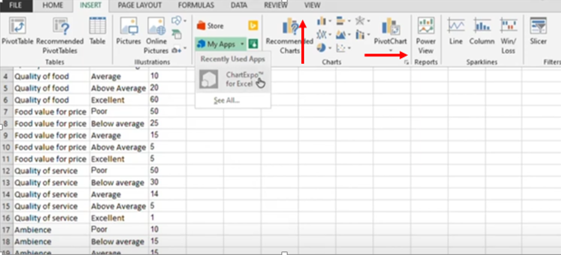
- Open the worksheet and click on the INSERT menu.
- You’ll see the My Apps option.
- Click the My Apps option and then click the See All button.

- Search for ChartExpo Add-in in the my Apps Store
- Click the Insert button.

- The add-in will be added to your Excel application.
- Log in with your Microsoft account or create a new account by clicking the Create one!
- Log in with the newly created account and start using the ChartExpo add-in to access advanced Excel charts.
- Enter your newly created account and start using the ChartExpo add-in. You’re only required to log in for the first time. Next time, ChartExpo won’t ask for your details again.
- Now you can start using ChartExpo and enjoy unlimited access to the best charts in Excel.

You will find 6 unique categories of data visualizations.

5 Advanced Excel Charts You Can Create Using ChartExpo
Let’s talk about the top 5 best charts in Excel you can create using ChartExpo.
1-Comparison Bar Chart
A Comparison Bar Chart is one of the best charts in Excel you can use to compare the metrics in your data with respect to dimensions, such as time.
You can only access this chart template once you’ve installed ChartExpo in your spreadsheet.
Benefits
You can use this chart to compare the performance of metrics in your data in different periods easily.
How to Create a Comparison Bar Chart?
Like we said, a Comparison Bar Chart is one of the best advanced Excel charts you can use to create persuasive data narratives for your target audience.
Let’s use the tabular data below to get started with this advanced
Excel chart. This data is about students registered for the subjects in different years.
| Year | Subject | Count |
| 2018 | Introduction to Probability | 700 |
| 2018 | Calculus Applied | 250 |
| 2018 | Computer Science for Lawyers | 300 |
| 2018 | The Architectural Imagination | 600 |
| 2018 | Principle of Biochemistry | 600 |
| 2018 | Data Science: R Basics | 250 |
| 2018 | Introduction to Game Development | 800 |
| 2018 | Entrepreneurship in Emerging Economics | 800 |
| 2018 | Understanding Technology | 600 |
| 2018 | Using Python for Research | 400 |
| 2018 | Data Science: Productivity Tools | 350 |
| 2018 | Data Science: Inference and Modeling | 800 |
| 2018 | Data Science: Wrangling | 250 |
| 2018 | Data Science: Linear Regression | 700 |
| 2019 | Introduction to Probability | 300 |
| 2019 | Calculus Applied | 350 |
| 2019 | Computer Science for Lawyers | 200 |
| 2019 | The Architectural Imagination | 350 |
| 2019 | Principle of Biochemistry | 800 |
| 2019 | Data Science: R Basics | 400 |
| 2019 | Introduction to Game Development | 650 |
| 2019 | Entrepreneurship in Emerging Economics | 550 |
| 2019 | Understanding Technology | 700 |
| 2019 | Using Python for Research | 250 |
| 2019 | Data Science: Productivity Tools | 500 |
| 2019 | Data Science: Inference and Modeling | 700 |
| 2019 | Data Science: Wrangling | 450 |
| 2019 | Data Science: Linear Regression | 500 |
| 2020 | Introduction to Probability | 700 |
| 2020 | Calculus Applied | 180 |
| 2020 | Computer Science for Lawyers | 250 |
| 2020 | The Architectural Imagination | 180 |
| 2020 | Principle of Biochemistry | 300 |
| 2020 | Data Science: R Basics | 500 |
| 2020 | Introduction to Game Development | 700 |
| 2020 | Entrepreneurship in Emerging Economics | 600 |
| 2020 | Understanding Technology | 300 |
| 2020 | Using Python for Research | 450 |
| 2020 | Data Science: Productivity Tools | 600 |
| 2020 | Data Science: Inference and Modeling | 600 |
| 2020 | Data Science: Wrangling | 500 |
| 2020 | Data Science: Linear Regression | 300 |
- Copy the table in Excel to get started with the Comparison Bar Chart.
- Click the Insert button to access the My Apps option.
- Click the My Apps option to see the ChartExpo add-in.
- You’ll see a library of charts categorized into 6 major sub-groups, as shown.
- Click the Comparative Analysis Charts button to access the Comparison Bar Chart, as shown.

- Select the Sheet holding the data and click Create Chart From Selection, as shown.

- Let’s have a zoom look on this chart.

Insights
The subject with the highest enrollment rate in 2020 is “Introduction to Game Development,” up from 4th in 2019 and 3rd position in 2018.
Conversely, “Computer Science for Lawyers” has the lowest enrollment rate across the 3 periods (2018, 2019, and 2020).
2-Slope Chart
Slope Charts are simple graphs that quickly and directly show transitions, changes over time, absolute values, and even rankings. Besides, they’re also called Slope Graphs.
You can use this chart to show the before and after story of variables in your data.
Benefits
Slope Graphs can be useful when you have two time periods or points of comparison and want to show relative increases and decreases quickly across various categories between two data points.
How to Create a Slope Chart in Excel using ChartExpo Add-in?
Let’s use the tabular data below in our example to get you started with data storytelling using a Slope Chart.
| Period | Months | Measure |
| 2020 | January | 69 |
| 2020 | February | 34 |
| 2020 | March | 16 |
| 2020 | April | 28 |
| 2020 | May | 43 |
| 2020 | June | 56 |
| 2020 | July | 74 |
| 2020 | August | 29 |
| 2020 | September | 60 |
| 2020 | October | 75 |
| 2020 | November | 67 |
| 2020 | December | 45 |
| 2019 | January | 78 |
| 2019 | February | 43 |
| 2019 | March | 20 |
| 2019 | April | 35 |
| 2019 | May | 39 |
| 2019 | June | 67 |
| 2019 | July | 65 |
| 2019 | August | 35 |
| 2019 | September | 70 |
| 2019 | October | 65 |
| 2019 | November | 87 |
| 2019 | December | 50 |
- Copy the table in Excel to get started with Slope Charts.
- Click the Insert button to access the My Apps option.
- Click the My Apps option to get the ChartExpo add-in.

- You’ll see a library of charts categorized into 6 major sub-groups.
- Click the Pay-per-click (PPC) Chart button to access the Slope Chart, as shown.

- Select the Sheet holding the data and click Create Chart from Selection, as shown.

- Let’s have zoom look on this chart.

Insights
- October and July are the best-performing month of the financial year 2020.
- Nov, Jan, sept and Jun are slightly decreased in year 2020 as compared to previous.
- March and December remained same in both year.
3-Radar Chart
This chart gets its name from its shape. In other words, it looks like a spider web, in which variables are organized in different shapes.
The Radar Chart is one of the best charts in Excel, because it’s incredibly easy to understand and customize. Furthermore, you can show several metrics across a single dimension. Use Radar charts to uncover outliers and commonalities in your data.
Benefits
- Radar Charts are incredibly easy to understand.
- You can easily spot patterns and trends in your data using this advanced Excel chart.
- A Radar Diagram is one of the best charts in Excel for data storytelling.
So how can you get started with Radar Charts?
If you’ve already installed ChartExpo in your Excel, follow the steps below to get started. But, if you’ve not installed ChartExpo, follow the easy-to-follow instructions above to get started with this FREE add-on.
Let’s use the example below.
Imagine you run a beauty brand, and want to know the best and worst-sellers in a given financial year. The products in your inventory include face creams, skin lightening creams, and beauty creams.
Let’s use the table below for our scenario.
| Product | Month | Number of Orders |
| Face Cream | Dec | 80 |
| Face Cream | Nov | 65 |
| Face Cream | Oct | 75 |
| Face Cream | Sep | 80 |
| Face Cream | Aug | 90 |
| Face Cream | July | 85 |
| Face Cream | June | 65 |
| Face Cream | May | 70 |
| Face Cream | April | 80 |
| Face Cream | Mar | 93 |
| Face Cream | Feb | 99 |
| Face Cream | Jan | 80 |
| Skin Lightening Cream | Dec | 100 |
| Skin Lightening Cream | Nov | 60 |
| Skin Lightening Cream | Oct | 95 |
| Skin Lightening Cream | Sep | 75 |
| Skin Lightening Cream | Aug | 100 |
| Skin Lightening Cream | July | 60 |
| Skin Lightening Cream | June | 95 |
| Skin Lightening Cream | May | 75 |
| Skin Lightening Cream | April | 109 |
| Skin Lightening Cream | Mar | 80 |
| Skin Lightening Cream | Feb | 109 |
| Skin Lightening Cream | Jan | 75 |
| Beauty Cream | Dec | 50 |
| Beauty Cream | Nov | 55 |
| Beauty Cream | Oct | 51 |
| Beauty Cream | Sep | 40 |
| Beauty Cream | Aug | 45 |
| Beauty Cream | July | 30 |
| Beauty Cream | June | 39 |
| Beauty Cream | May | 45 |
| Beauty Cream | April | 56 |
| Beauty Cream | Mar | 39 |
| Beauty Cream | Feb | 48 |
| Beauty Cream | Jan | 44 |
- Copy the table in Excel to get started with Radar Charts (one of the best charts in Excel).
- Click the Insert button to access the My Apps option.
- Click the My Apps option to access the ChartExpo add-in.
- You’ll see a library of charts categorized into 6 major sub-groups, as shown.

- Select your sheet data and click the General Analysis Charts tab to access Radar Chart, as shown.

- Select data and click the Create Chart from Selection button to visualize data in Excel, as shown.

- Let’s have a zoom look on this chart.

Insights
Face cream performed well in February, March, and July. On the other hand, skin lightening products performed well during April, June, August, October, and December.
The beauty cream was the poorest performer. And this means there’s a need for an in-depth investigation to determine the reason for abysmal performance of the product throughout the financial year.
4-Matrix Chart
A Matrix Chart shares remarkable similarities with the traditional bar chart. But, the critical difference is that the bars in this chart are stacked on each other to enhance comparison and come with parallel to other data to make it easier to understand the differences.
We recommend this diagram, which is one of the best charts in Excel, if your goal is to extract high-level insights from your data.
Benefits
- A Matrix Chart is incredibly easy to read and understand, even for non-technical audiences.
- Use this chart to uncover high-level insights into your data.
How to Create a Matrix Chart in Excel using ChartExpo?
Let’s use the tabular data below to get started with this chart.
| Brand | Store | Period | Number of Orders |
| Adidas | Store-B | Current | 100 |
| Adidas | Store-B | Previous | 200 |
| Adidas | Store-C | Current | 450 |
| Adidas | Store-C | Previous | 600 |
| Adidas | Store-A | Previous | 400 |
| Adidas | Store-A | Current | 620 |
| Nike | Store-B | Current | 240 |
| Nike | Store-B | Previous | 400 |
| Nike | Store-C | Current | 70 |
| Nike | Store-C | Previous | 100 |
| Nike | Store-A | Previous | 500 |
| Nike | Store-A | Current | 300 |
| Tesco | Store-B | Current | 700 |
| Tesco | Store-B | Previous | 600 |
| Tesco | Store-C | Current | 500 |
| Tesco | Store-C | Previous | 300 |
| Tesco | Store-A | Previous | 1200 |
| Tesco | Store-A | Current | 800 |
| lucky brand | Store-B | Current | 150 |
| lucky brand | Store-B | Previous | 70 |
| lucky brand | Store-C | Current | 350 |
| lucky brand | Store-C | Previous | 250 |
| lucky brand | Store-A | Previous | 600 |
| lucky brand | Store-A | Current | 700 |
| Calvin Klein | Store-B | Current | 200 |
| Calvin Klein | Store-B | Previous | 150 |
| Calvin Klein | Store-C | Current | 60 |
| Calvin Klein | Store-C | Previous | 80 |
| Calvin Klein | Store-A | Previous | 200 |
| Calvin Klein | Store-A | Current | 250 |
| DIESEL | Store-B | Current | 800 |
| DIESEL | Store-B | Previous | 500 |
| DIESEL | Store-C | Current | 300 |
| DIESEL | Store-C | Previous | 600 |
| DIESEL | Store-A | Previous | 400 |
| DIESEL | Store-A | Current | 500 |
| DOCKERS | Store-B | Current | 250 |
| DOCKERS | Store-B | Previous | 200 |
| DOCKERS | Store-C | Current | 300 |
| DOCKERS | Store-C | Previous | 100 |
| DOCKERS | Store-A | Previous | 400 |
| DOCKERS | Store-A | Current | 350 |
| George | Store-B | Current | 700 |
| George | Store-B | Previous | 500 |
| George | Store-C | Current | 250 |
| George | Store-C | Previous | 300 |
| George | Store-A | Previous | 200 |
| George | Store-A | Current | 100 |
| SANMAR | Store-B | Current | 70 |
| SANMAR | Store-B | Previous | 100 |
| SANMAR | Store-C | Current | 40 |
| SANMAR | Store-C | Previous | 80 |
| SANMAR | Store-A | Previous | 150 |
| SANMAR | Store-A | Current | 80 |
- Copy the table in Excel to get started with the Matrix Chart.
- Click the Insert button to access the My Apps option.
- Click the My Apps option to get the ChartExpo add-in.
- You’ll see a library of charts categorized into 6 major sub-groups, as shown.
- Click the Pay-per-Click Charts button to access the Bar Stacked Comparison Chart, as shown.

- Select the data on the sheet and click Create Chart from Selection, as shown.


As soon as you click on the button chart will be ready.

- If you want to add additional information, such as heading and legend, click the Edit Chart Button.
- Once you’re done with changes, click the Apply and then the Save Changes button.

- After editing, your final chart should look like the one below.


Insights
- Store A: The best and worst-performing brands in current and previous periods are Tesco and Sanmar, respectively.
- Store B: Diesel is the best-performing brand in the current period. Conversely, Sanmar is the worst-performing product.
- Store C: There is a tie in best performance between Diesel and Adidas in the previous period. Sanmar remains to be the worst-selling product in the brand.
5-Stack Bar Chart
A Stacked Bar Diagram is one of the best charts in Excel you can use to visualize part-to-whole relationships in your data.
Each bar in this chart represents a whole. And segments inside each bar represent different parts or categories of the whole. Different colors are used strategically to illustrate parts-to-whole insights.
Benefits
-
Easy to Use to Uncover Hidden Insights
A Stacked Bar Diagram is one of the advanced Excel charts you can easily use to compare data points for in-depth, high-level insights. This chart empowers you to see the percentage of each data point compared to the total value.
-
Save a Ton of Hours Every Day.
Stacked Bar Charts can help you save a lot of hours because it’s incredibly easy to plot, primarily if you use ChartExpo.
How to Create a Stacked Bar Chart in Excel using ChartExpo?
Let’s use the sample data below to get started with Stacked Bar Charts.
| Team | Silver | Gold | Bronze |
| USA | 41 | 39 | 33 |
| Japan | 14 | 27 | 17 |
| Australia | 7 | 17 | 22 |
| Italy | 10 | 10 | 20 |
| Germany | 11 | 10 | 16 |
| France | 12 | 10 | 11 |
| Brazil | 6 | 7 | 8 |
| Cuba | 3 | 7 | 5 |
| Poland | 5 | 4 | 5 |
- Copy the table in Excel to get started with Stacked Bar Charts.
- Click the Insert button to get the My Apps option.
- Click the My Apps option to access the ChartExpo add-in.
- You’ll see a library of charts categorized into 6 major sub-groups, as shown.
- Click the General Analysis Charts button to access Stacked Bar Chart, as shown.

- Select the Sheet holding the data and click Create Chart from Selection, as shown.

- You can edit chart and then change the colors according to your need, you can put some headers also and finally give a different aesthetics to this chart as shown below.


Insights
- The United States has the highest number of medals (gold, silver, and bronze).
- Japan has the second-largest number of medals.
- Poland is the worst performer on the list.
FAQs:
Why is visualization so Powerful?
Data visualization is incredibly important, especially in today’s world. Besides, it applies to almost all the sectors of the economy, including art and entertainment. Data visualization helps you save time taken to crunch raw numbers manually for in-depth insights.
Besides, it helps our brains to make sense of raw data in visual form quickly and effectively.
What is chart visualization?
Data visualization is the graphical representation of raw data for insights. Some of the best charts in Excel to use are Radar, Line, Stacked Bar, Comparison Non Sentimental, and Bar Stack Comparison Charts, among others.
You can only access these advanced Excel charts via third-party add-ins, such as ChartExpo.
Wrap Up
Congratulations if you’ve read the blog up to this point.
As we said, to get the most out of your data, you need the best charts in Excel. Why?
You don’t want your readers (or target audiences) to struggle to interpret the meaning and context of your data narrative. Using the right advanced Excel charts will not only save a ton of time but also make your data story persuasive.
Accessing the best charts in Excel (top 5 charts we highlighted earlier) does not have to be a struggle or even time-intensive. You need an intuitive and easy-to-use add-in to supercharge your Excel.
The data visualization tool we recommend to our readers is ChartExpo because of its full stack of tools, namely, graph maker, chart templates, and a data widget library.
These functionalities are incredibly easy to use. And this means you don’t need uber technical skills, such as coding or programming skills.
ChartExpo produces charts that are incredibly insightful and easy to read, even for non-technical audiences. So you can EASILY create social media reports, sales reports, and goal projections with this tool.
ChartExpo add-in has everything you need to create a compelling data story for your target readers (and target audiences). Try ChartExpo today to get the most out of your data.
Chart tools comprise of two tabs DESIGN and FORMAT.
Step 1 − When you click on a chart, CHART TOOLS comprising of DESIGN and FORMAT tabs appear on the Ribbon.
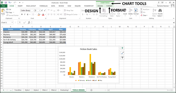
Step 2 − Click the DESIGN tab on the Ribbon. The Ribbon changes to the DESIGN commands.
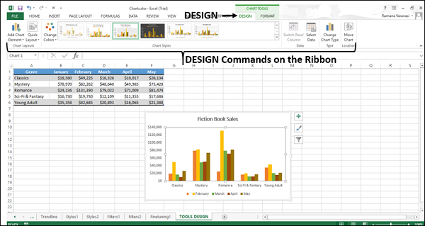
The Ribbon contains the following Design commands −
-
Chart layouts group
-
Add chart element
-
Quick layout
-
-
Chart styles group
-
Change colors
-
Chart styles
-
-
Data group
-
Switch row/column
-
Select data
-
-
Type group
-
Change chart type
-
-
Location group
-
Move chart
-
In this chapter, you will understand the design commands on the Ribbon.
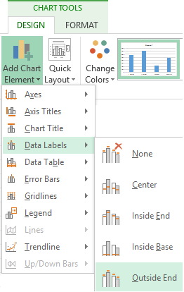
Add Chart Element
Add Chart Element is the same as chart elements.
Step 1 − Click Add Chart Element. The chart elements appear in the drop-down list. These are same as those in the chart elements list.
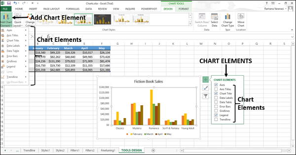
Refer to the chapter – Chart Elements in this tutorial.
Quick Layout
You can use Quick Layout to change the overall layout of the chart quickly by choosing one of the predefined layout options.
Step 1 − On the Ribbon, click Quick Layout. Different predefined layout options will be displayed.
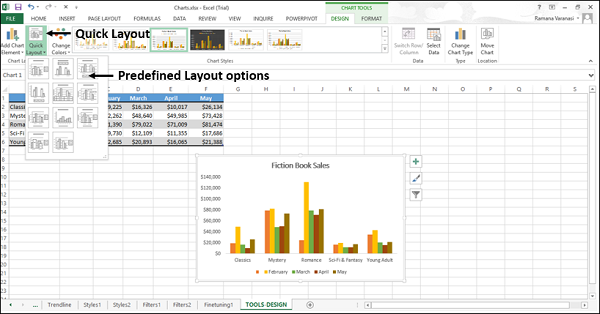
Step 2 − Move the pointer across the predefined layout options. The chart layout changes dynamically to the particular option.
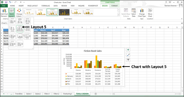
Step 3 − Select the layout you want. The chart will be displayed with the chosen layout.
Change Colors
The functions of Change Colors are the same as Chart Styles → COLOR.
Step 1 − On the Ribbon, click Change Colors. The color schemes appear in the drop-down list. These are the same as that appear in Change Styles → COLOR.
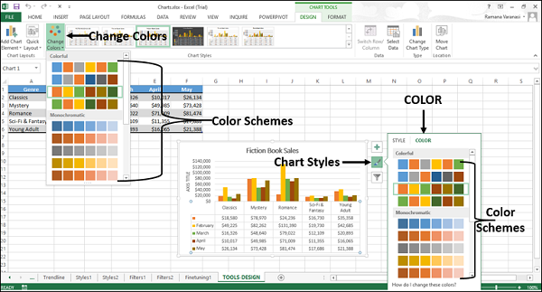
Refer to the chapter – Chart Styles in this tutorial.
Chart Styles
The Chart Styles command is the same as Chart Styles → STYLE.
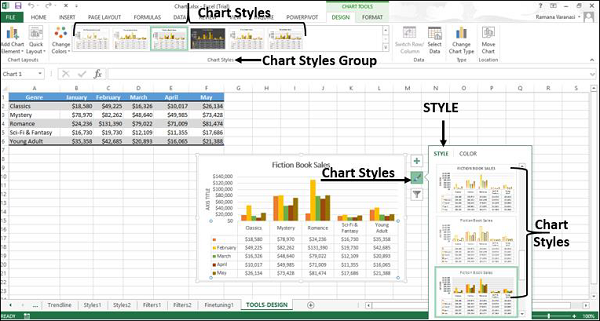
Refer to the chapter – Chart Styles in this tutorial.
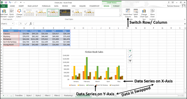
Switch Row/Column
You can use Switch Row/Column to change the data being displayed on X-axis to be displayed on Y-axis and vice versa.
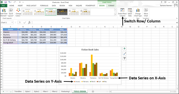
Click Switch Row / Column. The data will be swapped between X-axis and Y-axis on the chart.
Select Data
You can use Select Data to change the data range included in the chart.
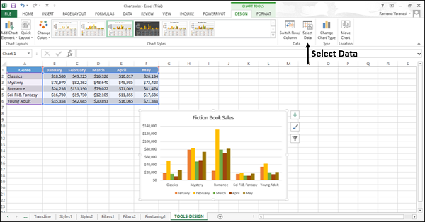
Step 1 − Click Select Data. A Select Data Source window appears.
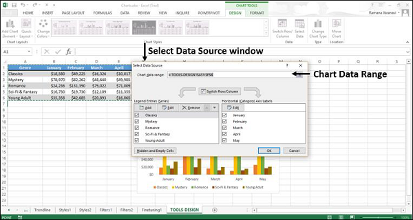
This window is the same as that appears with Chart Styles → Select data.
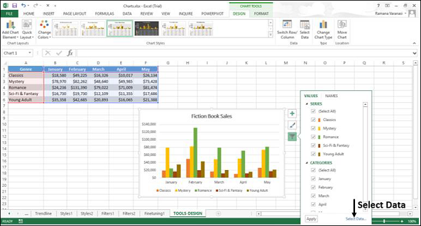
Step 2 − Select the chart data range in the select data source window.
Step 3 − Select the data that you want to display on your chart form the Excel worksheet.
Change Chart Type
You can use the Change Chart Type button to change your chart to a different chart type.
Step 1 − Click Change Chart Type. A Change Chart Type window appears.
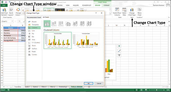
Step 2 − Select the chart type you want.
Your chart will be displayed with the chart type you want.
Move Chart
You can use Move Chart to move the chart to another worksheet in the workbook.
Step 1 − Click the Move Chart command button. A Move Chart window appears.
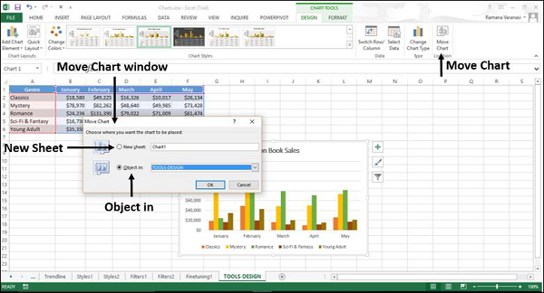
Step 2 − Select New Sheet. Type the name of the new sheet.
The chart moves from the existing sheet to the new sheet.
![]()
Gauge Chart Tool для Excel — абсолютно бесплатная надстройка для Microsoft Excel. Используя наш инструмент, вы можете создавать потрясающие графики как можно скорее.

-
AnyChart
AnyChart — это гибкая, кросс-платформенная и кросс-браузерная библиотека JavaScript-графиков, которая позволяет создавать интерактивные диаграммы HTML5, биржевые диаграммы, карты, диаграммы Ганта и информационные панели для любого проекта, в любом б…
Платно
Self-Hosted
Android
Linux
Mac
iPhone
Windows
Web
-
Ultimate Dashboard Tools for Excel
Ultimate Dashboard Tools — это профессиональное решение Excel для создания современных живых графиков и виджетов. Всегда в спешке? Мы рекомендуем нашу мощную надстройку. Создавайте потрясающие виджеты и специальные графики как можно скорее. Надстрой…
Платно
Microsoft Office Excel
Mac
Windows
-
Quick Dashboard Charts for Excel
Quick Dashboard Charts for Excel — это надстройка для Microsoft Office Excel В этой галерее представлены типы диаграмм Excel. Эта галерея содержит различные типы диаграмм, выбор которых показан ниже.
Платно
Microsoft Office Excel
Windows
-
think-cell chart
Диаграмма Think-Cell помогает создавать гистограммы, каскадные диаграммы, диаграммы Marimekko и диаграммы Ганта на слайдах презентаций Microsoft PowerPoint из таблиц данных Microsoft Excel.
Платно
Microsoft Office Excel
Microsoft Office Powerpoint
Windows
-
Mekko Graphics
Mekko Graphics предоставляет все необходимые вам функции построения графиков в одном простом пакете, который легко работает с Microsoft PowerPoint.
Платно
Microsoft Office Powerpoint
Windows
-
Peltier Tech Marimekko Chart Utility
Peltier Tech Marimekko Chart Utility — это надстройка для Microsoft Excel, которая позволяет быстро создавать диаграммы Marimekko.
Платно
Microsoft Office Excel
Mac
Windows
-
UpSlide
UpSlide быстро создала базу из более чем 450 команд в более чем 60 странах во всех отраслях. Тысячи клиентов используют UpSlide для создания миллионов совершенных и фирменных документов и отчетов каждый год, включая ведущие компании, такие как Sanof…
Платно
Word Online
Excel Online
Office Online
Power BI for Office 365
Powerpoint Online
Microsoft OneDrive
Microsoft SharePoint
Microsoft Office Excel
Microsoft Office 365
Microsoft Office Word
Microsoft Office Powerpoint
Windows
In this video, we’ll take a look at the tools that Excel provides for charting.
The number of tools Excel that provides for working with charts can be a little overwhelming. But the tools get easier with practice.
Let’s take a quick tour to get you acquainted.
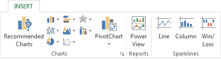
First, the ribbon.
To create a chart, you can click Recommended Charts on the Insert tab of the ribbon. Excel will show you recommended charts based on the data you’ve selected.
Alternately, if you know the chart type you want, you can use one of the small chart icons to the right.
Once you’ve created a chart, you’ll see two new tabs appear in the ribbon whenever the chart is selected: Design and Format. These appear under the Chart Tools heading.
When the chart is deselected, these tabs disappear.
In a nutshell, the Design tab has tools for adding chart elements, changing layouts, colors, chart styles, working with chart data, changing the chart type, and moving the chart.
The Format tab has tools for selecting and formatting chart elements, inserting shapes and text boxes, working with shape styles, applying wordart styles, and controls for changing layering, alignment, and chart size.
We’ll cover these features in more detail in upcoming videos.
Excel also attaches a menu of tools directly to the chart itself.
When you select a chart in Excel, you’ll see three helper icons to the right.
The plus icon helps you quickly add and remove common chart elements.
The paint brush icon allows you to apply chart styles and colors.
The filter icon allows you to quickly exclude or include chart data.
Also, when you right click a chart, you’ll see a context-sensitive menu appear with many useful options.
This menu changes to respond to the element selected, as you can see if I right click directly on different chart elements.
Above the context menu, you’ll see a mini toolbar.
The mini toolbar has a small set of common formatting options, and a menu to navigate top level chart elements.
To format text with the mini toolbar you’ll want to click once to select, then double click to get inside the text box.
Finally, in Excel 2013 and later, you’ll find the Format Task Pane. The Format Task Pane provides a huge array of options for configuring chart elements.
This intimidating control panel appears when you double click a chart element, or select a chart element and use the keyboard shortcut control + 1.
We’ll cover the Format Task Pane in more detail in upcoming videos.
Any information is easier to perceive when it’s represented in a visual form. It’s particularly relevant for numeric data that needs to be compared. In this case, charts are the optimal variant of representation. We will work in Excel.
Moreover, we will learn to create dynamic charts and graphs, which are updated automatically when you change the data. The link at the end of the article will allow you to download a sample template.
How to build a chart off a table in Excel?
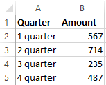
- Create a table with the data.
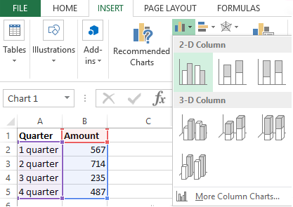
- Select the range of values A1:B5 that need to be presented as a chart. Go to the «INSERT» tab and choose the type.
- Click «Insert Column Chart» (as an example; you may choose a different type). Select one of the suggested bar charts.
- After you choose your bar chart type, it will be generated automatically.
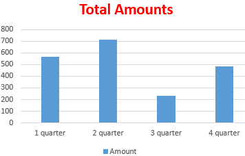
- Such a variant isn’t exactly what we need, so let’s modify it. Double-click on the bar chart’s title and enter «Total Amounts».
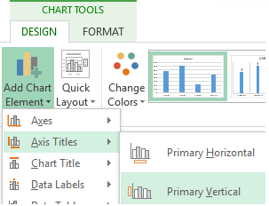
- Add the vertical axis title. Go to «CHART TOOLS» — «DESIGN» — «Add Element» — «Axis Titles» — «Primary Vertical». Select the vertical axis and its title type.
- Enter «AMOUNT».
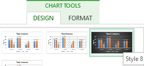
- Change the color and style. Choose a different style number 9.
- Specify the sums by giving titles to the bars. Go to the «DESIGN» tab, select «Data Labels» and the desired position.
Done!
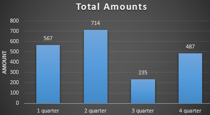
As a result, we have a stylish presentation of the data in Excel.
How to add data in an Excel chart?
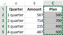
- Add new values to the table – the «Plan» column.
- Select the new range of values, including the heading. Copy it to the clipboard (by pressing Ctrl+C). Select the existing chart and paste the fragment (by pressing Ctrl+V).
- As it’s not entirely clear where the figures in our bar chart come from, let’s create the legend. Go to «DESIGN» — «Legend» — «Right». This is the result:
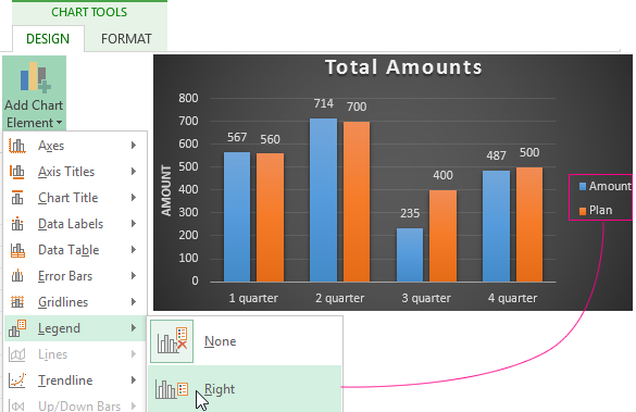
There is a more complicated way of adding new data into the existing graph through the «DESIGN» «Select Data» menu (open it by right-clicking and selecting «Select Data»).
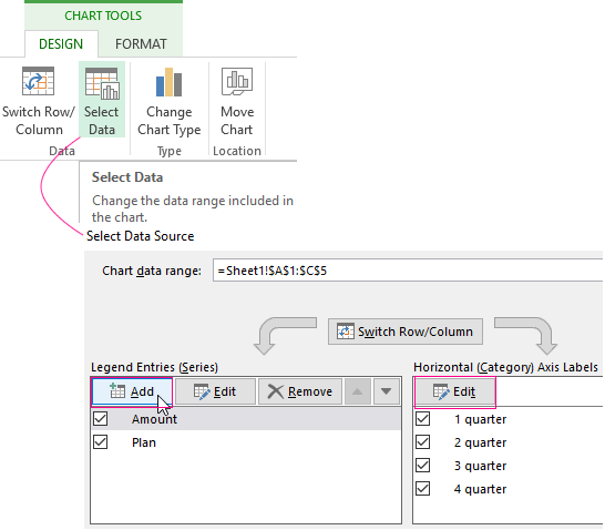
After you click «Add» (legend elements), there will open the row for selecting the range of values.
How to reverse axes in an Excel chart?
In the menu you’ve opened, click the «DESIGN»-«Switch/Column» button.
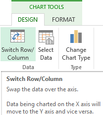
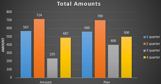
The values for rows and categories will swap around automatically.
How to lock controls in an Excel chart?
If you need to add new data in the bar chart very often, it’s not convenient to change the range every time. The optimal variant is to create a dynamic chart that will update automatically. To lock the controls, let’s transform the data range into a «Smart Table».
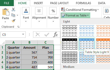
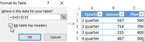
- Select the range of values A1:C5 and click «Format as Table» on «HOME» tab.
- Select any style in the drop-down menu. The program suggests you select the range for the table – agree with the suggested variant. The values for the graph will appear as follows:
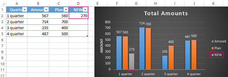
- As soon as you begin to enter new information in the table, the chart will also change. It has become dynamic:
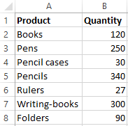
We have learned how to create a «Smart Table» off the existing data. If the spreadsheet is blank, start off with entering the values in the table: «INSERT» — «Table».
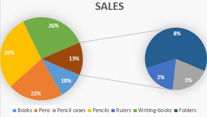
How to build a percentage chart in Excel?
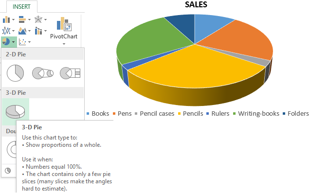
Pie charts are the best option for representing percentage information.
The input data for our sample chart:
- Select the range A1:B8. «INSERT» — «Insert Pie or Doughnut Chart» — «3D-Pie».
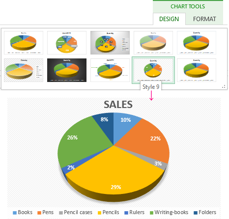
- Go to the tab «DESIGN» — «Styles». Among the suggested options, there are styles that include percentages. Choose the suitable 9.
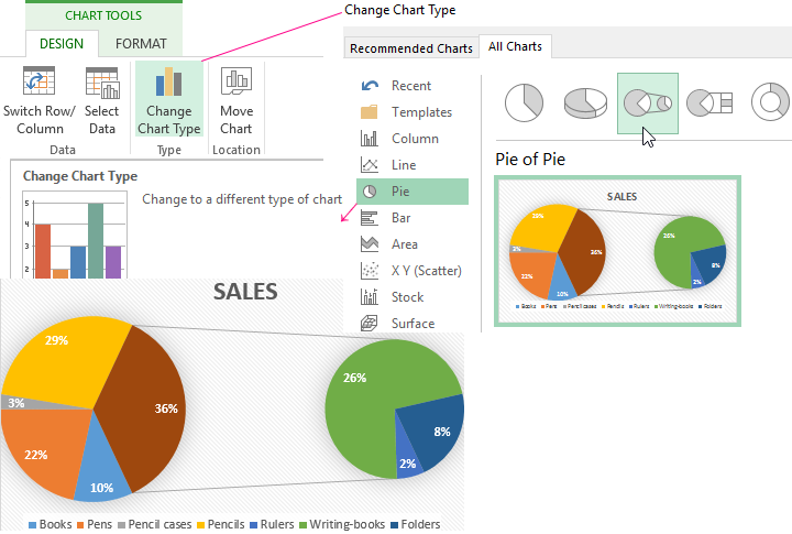
- The small percentage sectors are visible poorly. To highlight them, let’s create a secondary chart. Select the pie. Go to the tab «DESIGN» — «Change Chart Type». Select a pie with a secondary graph.
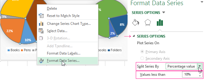
- The automatically generated option does not fulfill the task. Right-click on any sector. The dots designating the boundaries will become visible. Click «Format Data Series». Enter the following row parameters:
- We have obtained the desired variant:
Gantt chart in Excel
The Gantt chart is way of representing information in the form of bars to illustrate a multi-stage event. It’s a simple yet impressive trick.
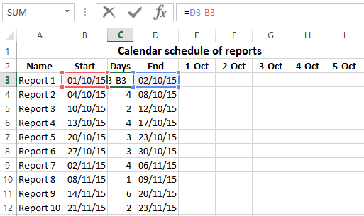
- We have a (dummy) table containing the deadlines for different reports.
- To create a chart, insert a column containing the number of days (column C). Fill it in with the help of Excel formulas.
- Select the range to contain the Gantt chart (E3:BF12). That is, the cells to be filled with a color between the beginning and end dates.
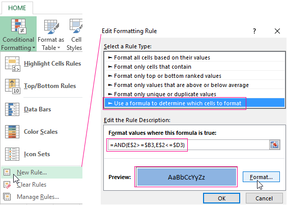
- Open the «Conditional Formatting» menu (on the «HOME» tab). Select «New Rule» — «Use a formula to determine which cells to format».
- Enter the formula of the following type: =AND(E$2>=$B3,E$2<=$D3). Excel uses the operator «И» to compare the date in the current cell with the beginning and end dates. Then, click «Format» and select the fill color.
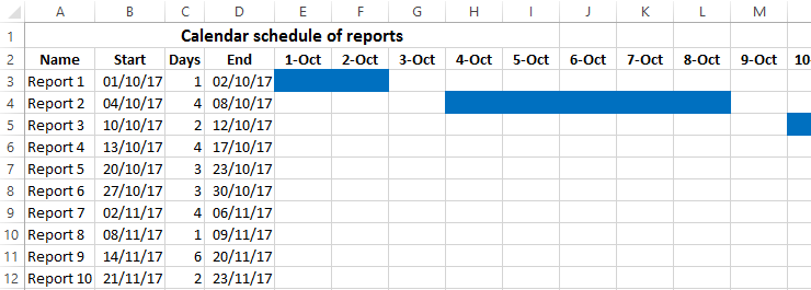
When you need to build a presentable financial report, it’s better to use the graphical data representation tools.
A simple Gantt graph is ready. You can also download the template with a sample:
Download all examples
If the information is represented in a graphical way, it’s perceived visually much quicker and more efficiently than texts and numbers. It makes it easier to conduct an analytic analysis. It makes the situation clearer – both the whole picture and particular details.
Charts and graphs were specifically developed in Excel for fulfilling such tasks.
Charts help you visualize your data in a way that creates maximum impact on your audience. Learn to create a chart and add a trendline. You can start your document from a recommended chart or choose one from our collection of pre-built chart templates.

Create a chart
-
Select data for the chart.
-
Select Insert > Recommended Charts.
-
Select a chart on the Recommended Charts tab, to preview the chart.
Note: You can select the data you want in the chart and press ALT + F1 to create a chart immediately, but it might not be the best chart for the data. If you don’t see a chart you like, select the All Charts tab to see all chart types.
-
Select a chart.
-
Select OK.
Add a trendline
-
Select a chart.
-
Select Design > Add Chart Element.
-
Select Trendline and then select the type of trendline you want, such as Linear, Exponential, Linear Forecast, or Moving Average.
Note: Some of the content in this topic may not be applicable to some languages.
Charts display data in a graphical format that can help you and your audience visualize relationships between data. When you create a chart, you can select from many chart types (for example, a stacked column chart or a 3-D exploded pie chart). After you create a chart, you can customize it by applying chart quick layouts or styles.
Charts contain several elements, such as a title, axis labels, a legend, and gridlines. You can hide or display these elements, and you can also change their location and formatting.
 Chart title
 Plot area
 Legend
 Axis titles
 Axis labels
 Tick marks
 Gridlines
You can create a chart in Excel, Word, and PowerPoint. However, the chart data is entered and saved in an Excel worksheet. If you insert a chart in Word or PowerPoint, a new sheet is opened in Excel. When you save a Word document or PowerPoint presentation that contains a chart, the chart’s underlying Excel data is automatically saved within the Word document or PowerPoint presentation.
Note: The Excel Workbook Gallery replaces the former Chart Wizard. By default, the Excel Workbook Gallery opens when you open Excel. From the gallery, you can browse templates and create a new workbook based on one of them. If you don’t see the Excel Workbook Gallery, on the File menu, click New from Template.
-
On the View menu, click Print Layout.
-
Click the Insert tab, and then click the arrow next to Chart.
-
Click a chart type, and then double-click the chart you want to add.
When you insert a chart into Word or PowerPoint, an Excel worksheet opens that contains a table of sample data.
-
In Excel, replace the sample data with the data that you want to plot in the chart. If you already have your data in another table, you can copy the data from that table and then paste it over the sample data. See the following table for guidelines for how to arrange the data to fit your chart type.
For this chart type
Arrange the data
Area, bar, column, doughnut, line, radar, or surface chart
In columns or rows, as in the following examples:
Series 1
Series 2
Category A
10
12
Category B
11
14
Category C
9
15
or
Category A
Category B
Series 1
10
11
Series 2
12
14
Bubble chart
In columns, putting x values in the first column and corresponding y values and bubble size values in adjacent columns, as in the following examples:
X-Values
Y-Value 1
Size 1
0.7
2.7
4
1.8
3.2
5
2.6
0.08
6
Pie chart
In one column or row of data and one column or row of data labels, as in the following examples:
Sales
1st Qtr
25
2nd Qtr
30
3rd Qtr
45
or
1st Qtr
2nd Qtr
3rd Qtr
Sales
25
30
45
Stock chart
In columns or rows in the following order, using names or dates as labels, as in the following examples:
Open
High
Low
Close
1/5/02
44
55
11
25
1/6/02
25
57
12
38
or
1/5/02
1/6/02
Open
44
25
High
55
57
Low
11
12
Close
25
38
X Y (scatter) chart
In columns, putting x values in the first column and corresponding y values in adjacent columns, as in the following examples:
X-Values
Y-Value 1
0.7
2.7
1.8
3.2
2.6
0.08
or
X-Values
0.7
1.8
2.6
Y-Value 1
2.7
3.2
0.08
-
To change the number of rows and columns included in the chart, rest the pointer on the lower-right corner of the selected data, and then drag to select additional data. In the following example, the table is expanded to include additional categories and data series.
-
To see the results of your changes, switch back to Word or PowerPoint.
Note: When you close the Word document or the PowerPoint presentation that contains the chart, the chart’s Excel data table closes automatically.
After you create a chart, you might want to change the way that table rows and columns are plotted in the chart. For example, your first version of a chart might plot the rows of data from the table on the chart’s vertical (value) axis, and the columns of data on the horizontal (category) axis. In the following example, the chart emphasizes sales by instrument.
However, if you want the chart to emphasize the sales by month, you can reverse the way the chart is plotted.
-
On the View menu, click Print Layout.
-
Click the chart.
-
Click the Chart Design tab, and then click Switch Row/Column.
If Switch Row/Column is not available
Switch Row/Column is available only when the chart’s Excel data table is open and only for certain chart types. You can also edit the data by clicking the chart, and then editing the worksheet in Excel.
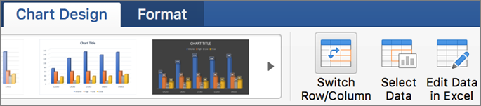
-
On the View menu, click Print Layout.
-
Click the chart.
-
Click the Chart Design tab, and then click Quick Layout.
-
Click the layout you want.
To immediately undo a quick layout that you applied, press
+ Z .
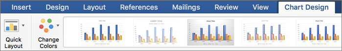
 + Z .
+ Z .Chart styles are a set of complementary colors and effects that you can apply to your chart. When you select a chart style, your changes affect the whole chart.
-
On the View menu, click Print Layout.
-
Click the chart.
-
Click the Chart Design tab, and then click the style you want.
To see more styles, point to a style, and then click
.To immediately undo a style that you applied, press
+ Z .
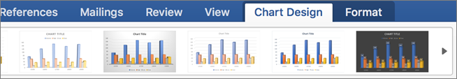
 .
.-
On the View menu, click Print Layout.
-
Click the chart, and then click the Chart Design tab.
-
Click Add Chart Element.
-
Click Chart Title to choose title format options, and then return to the chart to type a title in the Chart Title box.
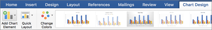
See also
Update the data in an existing chart
Chart types
Create a chart
You can create a chart for your data in Excel for the web. Depending on the data you have, you can create a column, line, pie, bar, area, scatter, or radar chart.
-
Click anywhere in the data for which you want to create a chart.
To plot specific data into a chart, you can also select the data.
-
Select Insert > Charts > and the chart type you want.
-
On the menu that opens, select the option you want. Hover over a chart to learn more about it.
Tip: Your choice isn’t applied until you pick an option from a Charts command menu. Consider reviewing several chart types: as you point to menu items, summaries appear next to them to help you decide.
-
To edit the chart (titles, legends, data labels), select the Chart tab and then select Format.
-
In the Chart pane, adjust the setting as needed. You can customize settings for the chart’s title, legend, axis titles, series titles, and more.

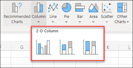
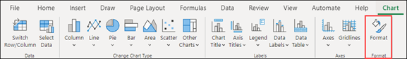

Available chart types
It’s a good idea to review your data and decide what type of chart would work best. The available types are listed below.
Data that’s arranged in columns or rows on a worksheet can be plotted in a column chart. A column chart typically displays categories along the horizontal axis and values along the vertical axis, like shown in this chart:

Types of column charts
-
Clustered column A clustered column chart shows values in 2-D columns. Use this chart when you have categories that represent:
-
Ranges of values (for example, item counts).
-
Specific scale arrangements (for example, a Likert scale with entries, like strongly agree, agree, neutral, disagree, strongly disagree).
-
Names that are not in any specific order (for example, item names, geographic names, or the names of people).
-
-
Stacked column A stacked column chart shows values in 2-D stacked columns. Use this chart when you have multiple data series and you want to emphasize the total.
-
100% stacked column A 100% stacked column chart shows values in 2-D columns that are stacked to represent 100%. Use this chart when you have two or more data series and you want to emphasize the contributions to the whole, especially if the total is the same for each category.
Data that is arranged in columns or rows on a worksheet can be plotted in a line chart. In a line chart, category data is distributed evenly along the horizontal axis, and all value data is distributed evenly along the vertical axis. Line charts can show continuous data over time on an evenly scaled axis, and are therefore ideal for showing trends in data at equal intervals, like months, quarters, or fiscal years.

Types of line charts
-
Line and line with markers Shown with or without markers to indicate individual data values, line charts can show trends over time or evenly spaced categories, especially when you have many data points and the order in which they are presented is important. If there are many categories or the values are approximate, use a line chart without markers.
-
Stacked line and stacked line with markers Shown with or without markers to indicate individual data values, stacked line charts can show the trend of the contribution of each value over time or evenly spaced categories.
-
100% stacked line and 100% stacked line with markers Shown with or without markers to indicate individual data values, 100% stacked line charts can show the trend of the percentage each value contributes over time or evenly spaced categories. If there are many categories or the values are approximate, use a 100% stacked line chart without markers.
Notes:
-
Line charts work best when you have multiple data series in your chart—if you only have one data series, consider using a scatter chart instead.
-
Stacked line charts add the data, which might not be the result you want. It might not be easy to see that the lines are stacked, so consider using a different line chart type or a stacked area chart instead.
-
Data that is arranged in one column or row on a worksheet can be plotted in a pie chart. Pie charts show the size of items in one data series, proportional to the sum of the items. The data points in a pie chart are shown as a percentage of the whole pie.

Consider using a pie chart when:
-
You have only one data series.
-
None of the values in your data are negative.
-
Almost none of the values in your data are zero values.
-
You have no more than seven categories, all of which represent parts of the whole pie.
Data that is arranged in columns or rows only on a worksheet can be plotted in a doughnut chart. Like a pie chart, a doughnut chart shows the relationship of parts to a whole, but it can contain more than one data series.

Tip: Doughnut charts are not easy to read. You may want to use a stacked column or stacked bar chart instead.
Data that is arranged in columns or rows on a worksheet can be plotted in a bar chart. Bar charts illustrate comparisons among individual items. In a bar chart, the categories are typically organized along the vertical axis, and the values along the horizontal axis.

Consider using a bar chart when:
-
The axis labels are long.
-
The values that are shown are durations.
Types of bar charts
-
Clustered A clustered bar chart shows bars in 2-D format.
-
Stacked bar Stacked bar charts show the relationship of individual items to the whole in 2-D bars
-
100% stacked A 100% stacked bar shows 2-D bars that compare the percentage that each value contributes to a total across categories.
Data that is arranged in columns or rows on a worksheet can be plotted in an area chart. Area charts can be used to plot change over time and draw attention to the total value across a trend. By showing the sum of the plotted values, an area chart also shows the relationship of parts to a whole.

Types of area charts
-
Area Shown in 2-D format, area charts show the trend of values over time or other category data. As a rule, consider using a line chart instead of a non-stacked area chart, because data from one series can be hidden behind data from another series.
-
Stacked area Stacked area charts show the trend of the contribution of each value over time or other category data in 2-D format.
-
100% stacked 100% stacked area charts show the trend of the percentage that each value contributes over time or other category data.
Data that is arranged in columns and rows on a worksheet can be plotted in an scatter chart. Place the x values in one row or column, and then enter the corresponding y values in the adjacent rows or columns.
A scatter chart has two value axes: a horizontal (x) and a vertical (y) value axis. It combines x and y values into single data points and shows them in irregular intervals, or clusters. Scatter charts are typically used for showing and comparing numeric values, like scientific, statistical, and engineering data.

Consider using a scatter chart when:
-
You want to change the scale of the horizontal axis.
-
You want to make that axis a logarithmic scale.
-
Values for horizontal axis are not evenly spaced.
-
There are many data points on the horizontal axis.
-
You want to adjust the independent axis scales of a scatter chart to reveal more information about data that includes pairs or grouped sets of values.
-
You want to show similarities between large sets of data instead of differences between data points.
-
You want to compare many data points without regard to time — the more data that you include in a scatter chart, the better the comparisons you can make.
Types of scatter charts
-
Scatter This chart shows data points without connecting lines to compare pairs of values.
-
Scatter with smooth lines and markers and scatter with smooth lines This chart shows a smooth curve that connects the data points. Smooth lines can be shown with or without markers. Use a smooth line without markers if there are many data points.
-
Scatter with straight lines and markers and scatter with straight lines This chart shows straight connecting lines between data points. Straight lines can be shown with or without markers.
Data that is arranged in columns or rows on a worksheet can be plotted in a radar chart. Radar charts compare the aggregate values of several data series.

Type of radar charts
-
Radar and radar with markers With or without markers for individual data points, radar charts show changes in values relative to a center point.
-
Filled radar In a filled radar chart, the area covered by a data series is filled with a color.
Add or edit a chart title
You can add or edit a chart title, customize its look, and include it on the chart.
-
Click anywhere in the chart to show the Chart tab on the ribbon.
-
Click Format to open the chart formatting options.
-
In the Chart pane, expand the Chart Title section.
-
Add or edit the Chart Title to meet your needs.
-
Use the switch to hide the title if you don’t want your chart to show a title.
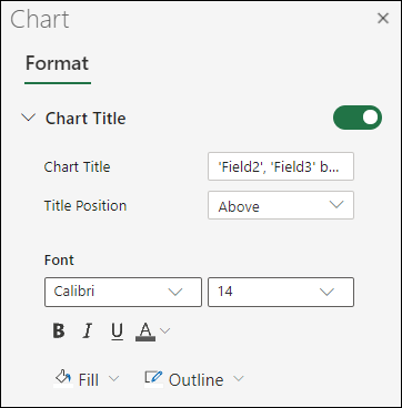
Add axis titles to improve chart readability
Adding titles to the horizontal and vertical axes in charts that have axes can make them easier to read. You can’t add axis titles to charts that don’t have axes, such as pie and doughnut charts.
Much like chart titles, axis titles help the people who view the chart understand what the data is about.
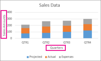
-
Click anywhere in the chart to show the Chart tab on the ribbon.
-
Click Format to open the chart formatting options.
-
In the Chart pane, expand the Horizontal Axis or Vertical Axis section.
-
Add or edit the Horizontal Axis or Vertical Axis options to meet your needs.
-
Expand the Axis Title.
-
Change the Axis Title and modify the formatting.
-
Use the switch to show or hide the title.
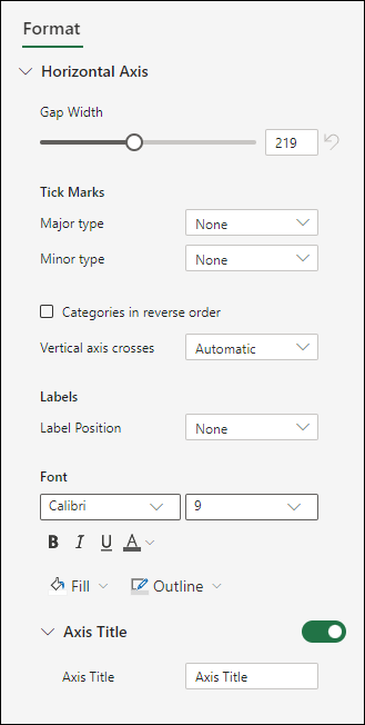

Change the axis labels
Axis labels are shown below the horizontal axis and next to the vertical axis. Your chart uses text in the source data for these axis labels.

To change the text of the category labels on the horizontal or vertical axis:
-
Click the cell which has the label text you want to change.
-
Type the text you want and press Enter.
The axis labels in the chart are automatically updated with the new text.
Tip: Axis labels are different from axis titles you can add to describe what is shown on the axes. Axis titles aren’t automatically shown in a chart.
Remove the axis labels
To remove labels on the horizontal or vertical axis:
-
Click anywhere in the chart to show the Chart tab on the ribbon.
-
Click Format to open the chart formatting options.
-
In the Chart pane, expand the Horizontal Axis or Vertical Axis section.
-
From the dropdown box for Label Position, select None to prevent the labels from showing on the chart.

Need more help?
You can always ask an expert in the Excel Tech Community or get support in the Answers community.