Changing an array in excel

You’re trying to edit an array formula, and you’re stopped in your tracks. You click the formula in the cell or formula bar and you can’t change a thing. Array formulas are a special case, so do one of the following:

If you’ve entered a single-cell array formula, select the cell, press F2, make your changes, and then press Ctrl+Shift+Enter..

If you’ve entered a multi-cell array formula, select all the cells that contain it, press F2, and follow these rules:

• You can’t move the individual cells that contain your formula, but you can move all of them as a group, and the cell references in the formula will change with them. To move them, select all the cells, press Ctrl+X, select the new location and press Ctrl+V.

• You can’t delete cells in an array formula (you’ll see a «You cannot change part of an array» error), but you can delete the entire formula and start over.

• You can’t add new cells to a block of result cells, but you can add new data to your worksheet and then expand your formula.

• After you make your changes, press Ctrl+Shift+Enter.

Finally, you may be able to save time if you use array constants—parts of an array formula that you type in the formula bar. But, they also have a few editing and usage rules. For more about them, see Use array constants in array formulas.

Can you edit an array in Excel?

To edit the contents of an array formula, follow these steps: Select a cell in the array range and then activate Edit mode by clicking the formula in the Formula bar or pressing F2. … Edit the array formula contents. Press Ctrl+Shift+Enter to enter your changes.

How do you change the range of an array in Excel?

Here’s what you need to do.

1. Select the range of cells that contains your current array formula, plus the empty cells next to the new data.
2. Press F2. Now you can edit the formula.
3. Replace the old range of data cells with the new one. …
4. Press Ctrl+Shift+Enter.

How do you edit an array in Excel 2016?

You click the formula in the cell or formula bar and you can’t change a thing. Array formulas are a special case, so do one of the following: If you’ve entered a single-cell array formula, select the cell, press F2, make your changes, and then press Ctrl+Shift+Enter..

How do you designate an array in Excel?

Creating an Array Formula

1. You need to click on cell in which you want to enter the array formula.
2. Begin the array formula with the equal sign and follow the standard formula syntax and use mathematical operators or built in functions in Excel formula, as required. …
3. Press Ctrl+Shift+Enter to produce the desired result.

How do you fill down an array in Excel?

Press the keyboard shortcut CTRL + SHIFT + ENTER to complete the array formula. Once you do this, Microsoft Excel surrounds the formula with {curly braces}, which is a visual indication of an array formula.

How do you fix can’t change part of an array in Excel?

What is array function in Excel?

An array formula is a formula that can perform multiple calculations on one or more items in an array. You can think of an array as a row or column of values, or a combination of rows and columns of values. Array formulas can return either multiple results, or a single result.

How do you make a dynamic array in Excel?

A dynamic array formula is entered in one cell and completed with a regular Enter keystroke. To complete an old-fashioned array formula, you need to press Ctrl + Shift + Enter. New array formulas spill to many cells automatically. CSE formulas must be copied to a range of cells to return multiple results.

Is array sequential or random?

Elements stored in an array can be accessed both sequentially and randomly. * An array is a contiguous collection of elements that can be accessed randomly by the means of their index value. * This is known as random access of the array elements using an index. This is also known as a dynamic array.

What is array give the example?

An array is a data structure that contains a group of elements. … For example, a search engine may use an array to store Web pages found in a search performed by the user. When displaying the results, the program will output one element of the array at a time.

What is Ctrl enter in Excel?

#2 – Ctrl+Enter to Fill All Selected Cells with the Same Data or Formula. When we are entering data or a formula in a cell, and have multiple cells selected, Ctrl+Enter will copy the data/formula to all of the selected cells.

What is {} in Excel?

A CSE formula in Excel is an array formula that must be entered with control + shift + enter. When a formula is entered with CSE, Excel automatically wraps the formula in curly braces {}.

What are some examples of arrays?

An array is a variable that can store multiple values. For example, if you want to store 100 integers, you can create an array for it. int data[100];

What are the types of array?

There are three different kinds of arrays: indexed arrays, multidimensional arrays, and associative arrays.

What is the right way to initialization array?

Solution(By Examveda Team)

Only square brackets([]) must be used for declaring an array.

How can we describe an array in the best possible way?

02. How can we describe an array in the best possible way? Explanation: The array stores the elements in a contiguous block of memory of similar types. Therefore, we can say that array is a container that stores elements of similar types.

How do I input an array into a single line?

values is one char , so your array has exactly one element. You should use std::vector<int> and push_back . (Examples are all over the internet.)

How do you define an array?

An array is a collection of elements of the same type placed in contiguous memory locations that can be individually referenced by using an index to a unique identifier. Five values of type int can be declared as an array without having to declare five different variables (each with its own identifier).

What are the disadvantages of arrays *?

Disadvantages of arrays:

• The number of elements to be stored in arrays should be known beforehand.
• An array is static.
• Insertion and deletion is quite difficult in an array.
• Allocating more memory than required leads to wastage of memory.

Does an array have a fixed length?

An array is a container object that holds a fixed number of values of a single type. The length of an array is established when the array is created. After creation, its length is fixed.

What is the starting index of an array?

In computer science, array indices usually start at 0 in modern programming languages, so computer programmers might use zeroth in situations where others might use first, and so forth.

What are the advantages of arrays *?

1) Array stores data elements of the same data type. 2) Maintains multiple variable names using a single name. Arrays help to maintain large data under a single variable name. This avoid the confusion of using multiple variables.

What is the difference between array and array list?

Array is a fixed length data structure whereas ArrayList is a variable length Collection class. We cannot change length of array once created in Java but ArrayList can be changed. We cannot store primitives in ArrayList, it can only store objects. But array can contain both primitives and objects in Java.

What is array advantages and disadvantages?

It allows us to enter only fixed number of elements into it. We cannot alter the size of the array once array is declared. Hence if we need to insert more number of records than declared then it is not possible.

What is multidimensional array example?

A multi-dimensional array is an array with more than one level or dimension. For example, a 2D array, or two-dimensional array, is an array of arrays, meaning it is a matrix of rows and columns (think of a table). A 3D array adds another dimension, turning it into an array of arrays of arrays.

What is array and its limitations?

The limitations of an array are explained below − An array which is formed will be homogeneous. That is, in an integer array only integer values can be stored, while in a float array only floating value and character array can have only characters. Thus, no array can have values of two data types.

How are linked lists better than arrays?

Better use of Memory:

From a memory allocation point of view, linked lists are more efficient than arrays. Unlike arrays, the size for a linked list is not pre-defined, allowing the linked list to increase or decrease in size as the program runs.

What is multidimensional array explain?

A multidimensional array in MATLAB® is an array with more than two dimensions. In a matrix, the two dimensions are represented by rows and columns. Each element is defined by two subscripts, the row index and the column index.

Does your Excel showing you cannot change part of an array error? But you don’t have any idea why you are getting this error and how to fix this?

Well, in that case, this blog is really gonna help you a lot. As it covers detailed information on Excel error you cannot change part of an array and ways to resolve this.

What Does You Can’t Change Part Of An Array Mean?

Excel array formula is one such formula that can execute multiple calculations over single or multiple numbers of items in the array.

You can consider this array as the combination of value’s rows and columns. Array formula can give you single or multiple results in return.

Suppose, in the range of cells you can also make the array formulas and can use the array formula for calculating column or row. Just place the array formula within a single cell for making the calculation of a single amount.

Array formula which is having multiple cells is known as a multi-cell formula. Whereas, the array formula present in the single-cell is known as the single-cell formula.

This Excel error you can’t change part of an array arises due to the issue in the range of array formula. Now you need to choose entire cells from that array before making any changes to it.

Here is the screenshot of this error:

Method 1# Match The Syntax

Usually, the array formulas strictly follow the standard formula syntax. It starts with an equal sign.

In the array formulas, you can use the Excel built-in functions. So, make a press over the Ctrl+Shift+Enter for entering the formula.

Excel closes array formula within the braces. But if you manually add these braces then the array formula will get converted to the text string and this won’t work correctly.

To build a complex formula, Array functions are quite an efficient option to choose from.

Suppose you are using complex formula like this: =SUM(C2*D2,C3*D3,C4*D4,C5*D5,C6*D6,C7*D7,C8*D8,C9*D9,C10*D10,C11*D11).

 So instead of using the above complex formula, you can use the array formula =SUM(C2:C11*D2:D11)

Method 2# Rules For Changing Array Formulas

If you are rigorously trying to make changes in the formula bar or in the formula cell. But every time you are getting the same you cannot change part of an array error.

In that case, quickly make a cross-check over the below-mentioned array formula guidelines.

Breaking the rules for changing array formulas also results in you cannot change part of an array error.

• If you are entering a single-cell array formula, then choose the cell and hit the F2 button to make easy changes.
• After that press the Ctrl+Shift+Enter button from your keyboard.
• If in case, you are entering the multi-cell array formula then choose the entire cell having this formula and then press the F2 button. after that below mentioned set of rules:
• You are not allowed to move individual cells having the formula, but as a group, you can all of them at once. Ding this will automatically change the formula cell references accordingly.

To shift this to a new place, choose the entire cell and press the Ctrl+X.  Choose any new location, where you want to paste it. After that make a press over the Ctrl+V button.

• In the array formula, you can’t delete any cells if you are trying to do so then it’s obvious to get the “You cannot change part of an array”

But you have the option to delete the complete formula and then start again from the beginning.

• Nor, you can’t add new cells to the section of result cells. But you have the option to add new data within your Excel worksheet and then expand the array formulas.
• After doing complete changes, hit the Ctrl+Shift+Enter.

Using the array constants (part of array formula which is typed in formula bar) you can easily save up your time. But remember one thing that array constants also have a few usage and editing rules.

Method 3# Use Ctrl+Shift+Enter

It is the basic and most important component of array formulas which you need to enter by using the Ctrl+Shift+Enter.

Here are the steps to create an array formula:

• Choose cells that contain the array formula.
• Assign the formula either by typing or using the formula bar.
• After completing all these, enter the formula and then type Ctrl+Shift+Enter.
• Just put the formula within the array.

Method 4# Use Names To Refer To Arrays

One plus point about the Excel arrays is that it offers the option of including the named ranges. One can use these named ranges either in the time-series or to the table formulas which is enforced for using the cell references.

With the array formulas, you will see that your spreadsheet formula will be easier to read and interpret with named cells.

Method 5# Select Arrays With A Keyboard Shortcut

If you are working with an already existing cell array formula then it’s important to choose and edit the complete array.

It’s quite tedious but there are some shortcuts available to use this.

• To select the cell of array press the “Ctrl” and forward-slash (“/”). Similarly, you can select the entire array.
• Press the F2 key or you can edit the formula present within the formula bar.

Last but not least after completing all this just type Ctrl+Shift+Enter.

Method 6# Remove Part Of An Array In Excel

If the above fixes won’t resolve the error you cannot change part of an array then try removing some part of your array. Doing this will definitely going to work.

After deleting up the formula, you will see that result of the formula is also gets deleted. If you don’t want to remove the values then only remove the formula.

Learn how both these tasks should be performed.

Delete A Formula But Keep The Results

For deleting up the formula and keeping up the result you need to copy the formula after that paste it in the same cell. But this time you have to use the Paste Values option.

1. Choose the cell ranges or cells having the formulas in them. If you have used the array formula, then firstly you need to choose the cells present in the ranges of the cells having the array formula.

• Tap to the cell in the array formula.
• Hit the Home tab, and then from the Editing group, choose the Find & Select.

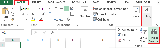
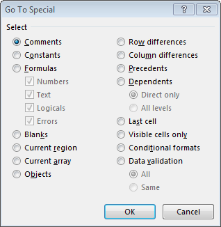
• After that tap to the Go To > Special > Current array.

2. Go to the Home tab and then from the Clipboard group, choose the Copy

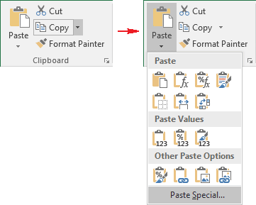
3. Go to the Home tab and then from the Clipboard group, tap the arrow present below the Paste button, and then hit the Paste Values.

Delete An Array Formula

For deleting up the array formula, choose all cells to present within the range of cells having the array formula in it. After that perform the following step:

• Tap to the cell present in the array formula.
• Go to the Home tab, in the Editing group, click Find & Select, and then click Go To.

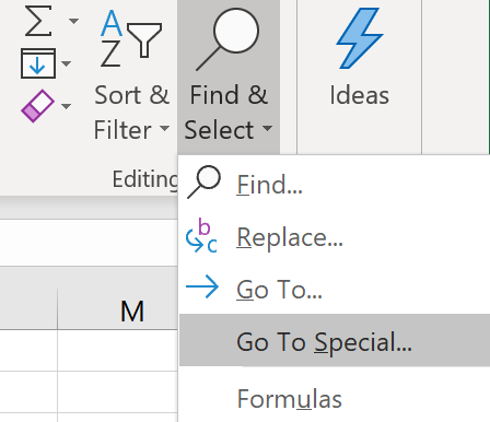
• Click Special>Current array

• At last hit the DELETE

Wrap Up:

Undoubtedly, using the Array formulas is a great option to use but it has disadvantages too. I have noticed the following points.

As per the processing speed and computer memory, large array formulas may result in slower calculation.

Other Excel workbook users maybe won’t understand the formula. Generally, array formulas are not explained within the worksheet.

So if any other user needs to edit the workbooks then it’s compulsory for them to have knowledge about array formulas or you need to avoid the array formulas.

Во время работы с таблицами Excel довольно часто приходится оперировать с целыми диапазонами данных. При этом некоторые задачи подразумевают, что вся группа ячеек должна быть преобразована буквально в один клик. В Экселе имеются инструменты, которые позволяют проводить подобные операции. Давайте выясним, как можно управлять массивами данных в этой программе.

Операции с массивами

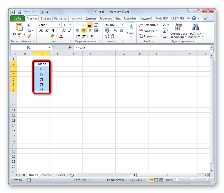
Массив – это группа данных, которая расположена на листе в смежных ячейках. По большому счету, любую таблицу можно считать массивом, но не каждый из них является таблицей, так как он может являться просто диапазоном. По своей сущности такие области могут быть одномерными или двумерными (матрицы). В первом случае все данные располагаются только в одном столбце или строке.

Во втором — в нескольких одновременно.

Кроме того, среди одномерных массивов выделяют горизонтальный и вертикальный тип, в зависимости от того, что они собой представляют – строку или столбец.

Нужно отметить, что алгоритм работы с подобными диапазонами несколько отличается от более привычных операций с одиночными ячейками, хотя и общего между ними тоже много. Давайте рассмотрим нюансы подобных операций.

Создание формулы

Формула массива – это выражение, с помощью которого производится обработка диапазона с целью получения итогового результата, отображаемого цельным массивом или в одной ячейке. Например, для того, чтобы умножить один диапазон на второй применяют формулу по следующему шаблону:

=адрес_массива1*адрес_массива2

Над диапазонами данных можно также выполнять операции сложения, вычитания, деления и другие арифметические действия.

Координаты массива имеют вид адресов первой её ячейки и последней, разделенные двоеточием. Если диапазон двумерный, то первая и последняя ячейки расположены по диагонали друг от друга. Например, адрес одномерного массива может быть таким: A2:A7.

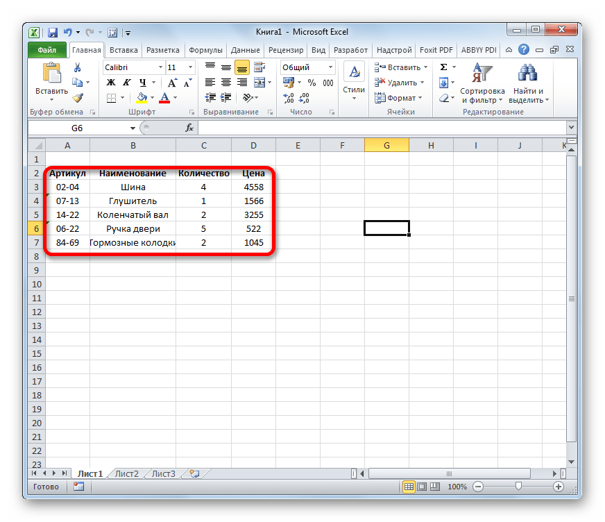
А пример адреса двумерного диапазона выглядит следующим образом: A2:D7.

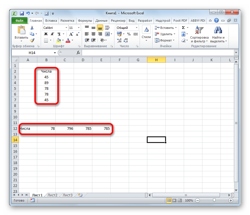
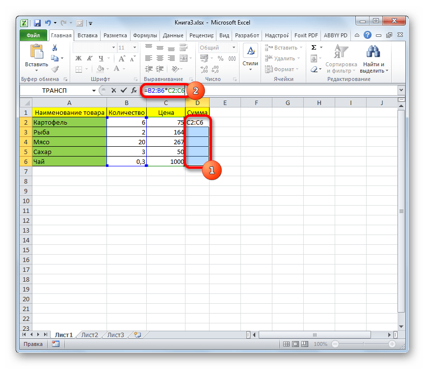
1. Чтобы рассчитать подобную формулу, нужно выделить на листе область, в которую будет выводиться результат, и ввести в строку формул выражение для вычисления.



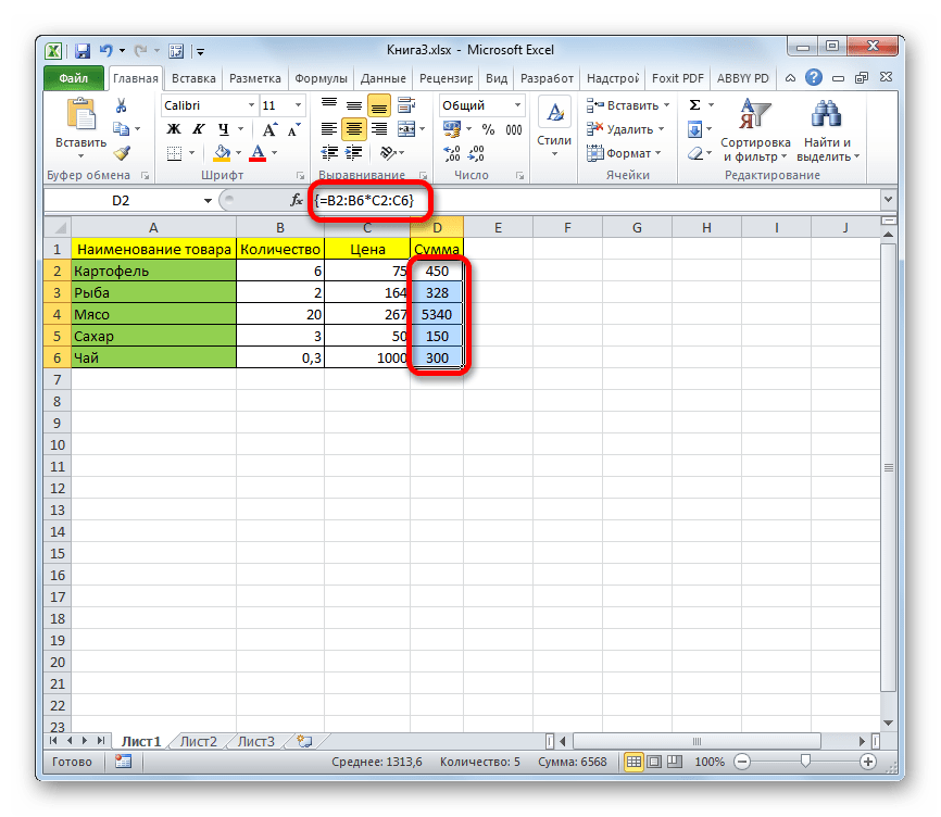
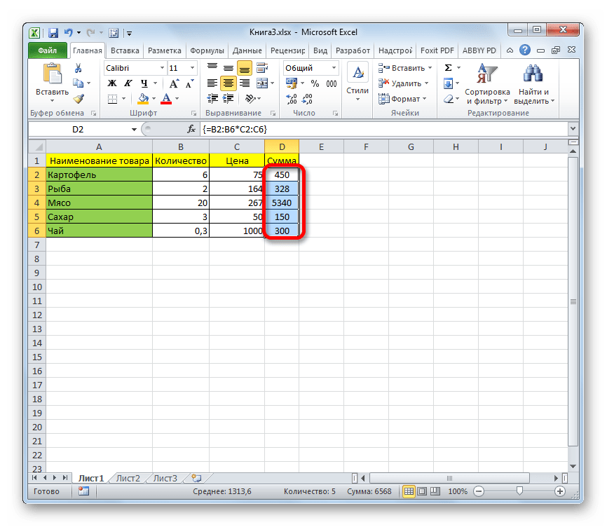
2. После ввода следует нажать не на кнопку Enter, как обычно, а набрать комбинацию клавиш Ctrl+Shift+Enter. После этого выражение в строке формул будет автоматически взято в фигурные скобки, а ячейки на листе будут заполнены данными, полученными в результате вычисления, в пределах всего выделенного диапазона.

Изменение содержимого массива

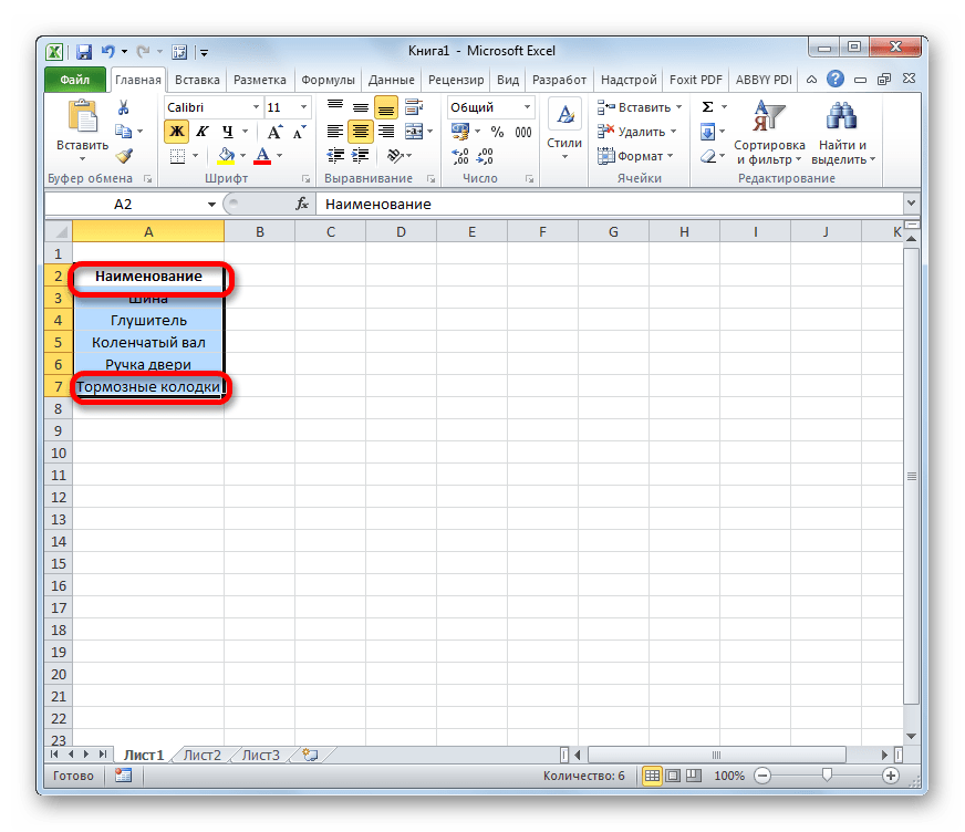
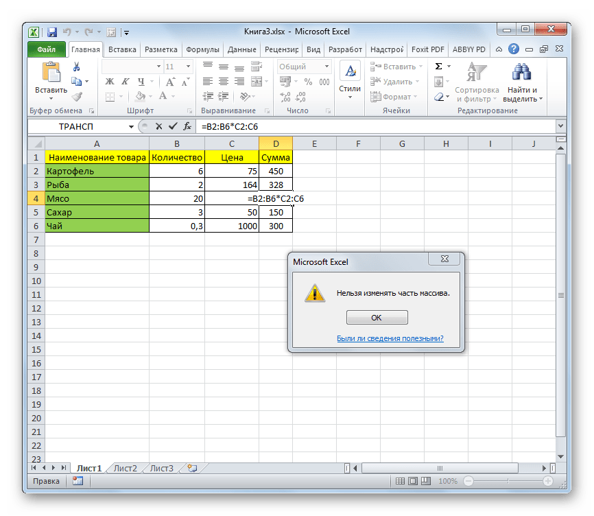
Если вы в дальнейшем попытаетесь удалить содержимое или изменить любую из ячеек, которая расположена в диапазоне, куда выводится результат, то ваше действие окончится неудачей. Также ничего не выйдет, если вы сделаете попытку отредактировать данные в строке функций. При этом появится информационное сообщение, в котором будет говориться, что нельзя изменять часть массива. Данное сообщение появится даже в том случае, если у вас не было цели производить какие-либо изменения, а вы просто случайно дважды щелкнули мышью по ячейке диапазона.

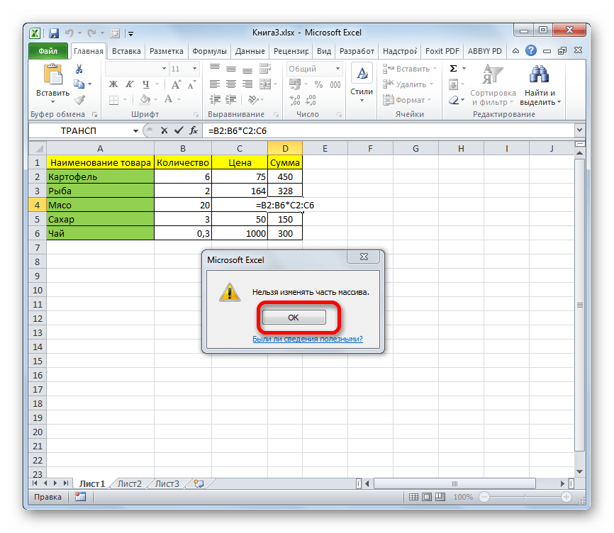
Если вы закроете, это сообщение, нажав на кнопку «OK», а потом попытаетесь переместить курсор с помощью мышки, или просто нажмете кнопку «Enter», то информационное сообщение появится опять. Не получится также закрыть окно программы или сохранить документ. Все время будет появляться это назойливое сообщение, которое блокирует любые действия. А выход из ситуации есть и он довольно прост

1. Закройте информационное окно, нажав на кнопку «OK».



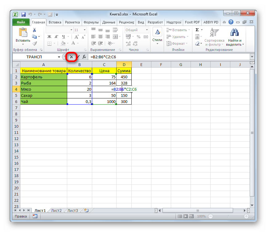
2. Затем нажмете на кнопку «Отмена», которая расположена в группе значков слева от строки формул, и представляет собой пиктограмму в виде крестика. Также можно нажать на кнопку Esc на клавиатуре. После любой из этих операций произойдет отмена действия, и вы сможете работать с листом так, как и прежде.

Но что делать, если действительно нужно удалить или изменить формулу массива? В этом случае следует выполнить нижеуказанные действия.

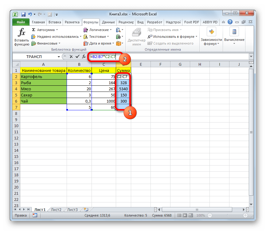
1. Для изменения формулы выделите курсором, зажав левую кнопку мыши, весь диапазон на листе, куда выводится результат. Это очень важно, так как если вы выделите только одну ячейку массива, то ничего не получится. Затем в строке формул проведите необходимую корректировку.



2. После того, как изменения внесены, набираем комбинацию Ctrl+Shift+Esc. Формула будет изменена.

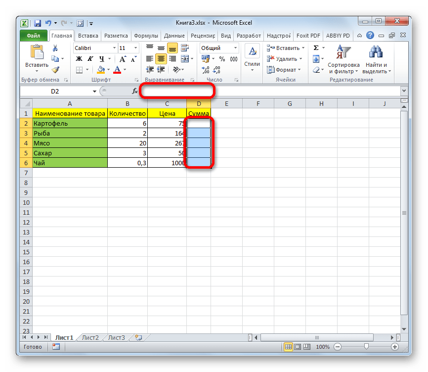
1. Для удаления формулы массива нужно точно так же, как и в предыдущем случае, выделить курсором весь диапазон ячеек, в котором она находится. Затем нажать на кнопку Delete на клавиатуре.



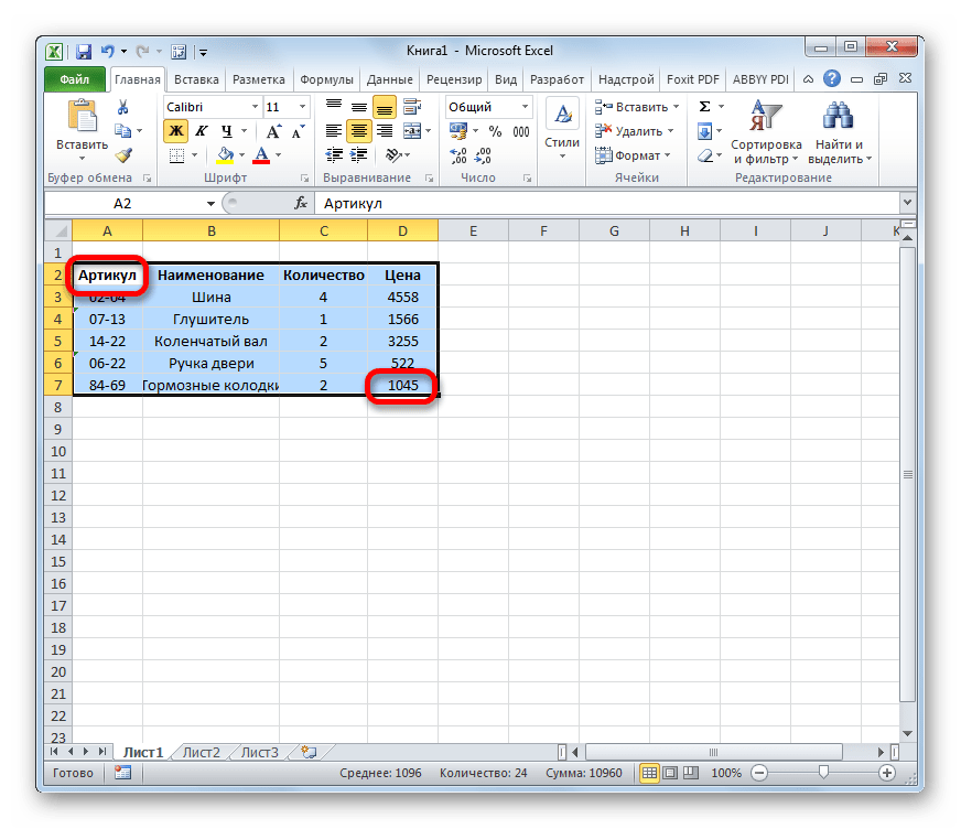
2. После этого формула будет удалена со всей области. Теперь в неё можно будет вводить любые данные.

Функции массивов

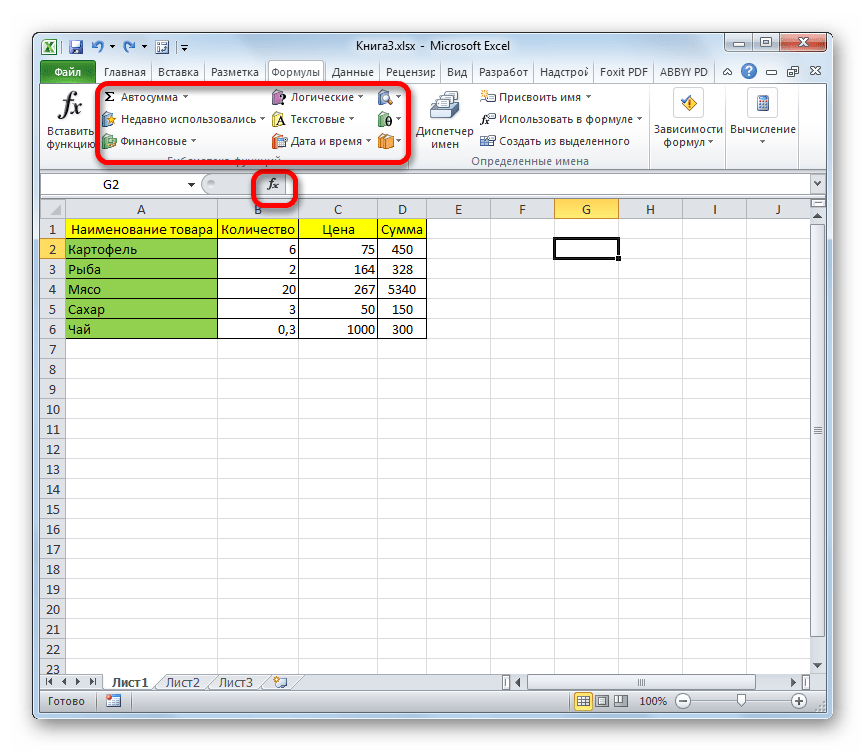
Наиболее удобно в качестве формул использовать уже готовые встроенные функции Excel. Доступ к ним можно получить через Мастер функций, нажав кнопку «Вставить функцию» слева от строки формул. Или же во вкладке «Формулы» на ленте можно выбрать одну из категорий, в которой находится интересующий вас оператор.

После того, как пользователь в Мастере функций или на ленте инструментов выберет наименование конкретного оператора, откроется окно аргументов функции, куда можно вводить исходные данные для расчета.

Правила ввода и редактирования функций, если они выводят результат сразу в несколько ячеек, те же самые, что и для обычных формул массива. То есть, после ввода значения обязательно нужно установить курсор в строку формул и набрать сочетание клавиш Ctrl+Shift+Enter.

Урок: Мастер функций в Excel

Оператор СУММ

Одной из наиболее востребованных функций в Экселе является СУММ. Её можно применять, как для суммирования содержимого отдельных ячеек, так и для нахождения суммы целых массивов. Синтаксис этого оператора для массивов выглядит следующим образом:

=СУММ(массив1;массив2;…)

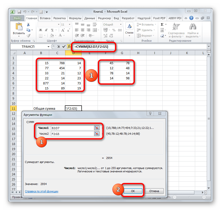
Данный оператор выводит результат в одну ячейку, а поэтому для того, чтобы произвести подсчет, после внесения вводных данных достаточно нажать кнопку «OK» в окне аргументов функции или клавишу Enter, если ввод выполнялся вручную.

Урок: Как посчитать сумму в Экселе

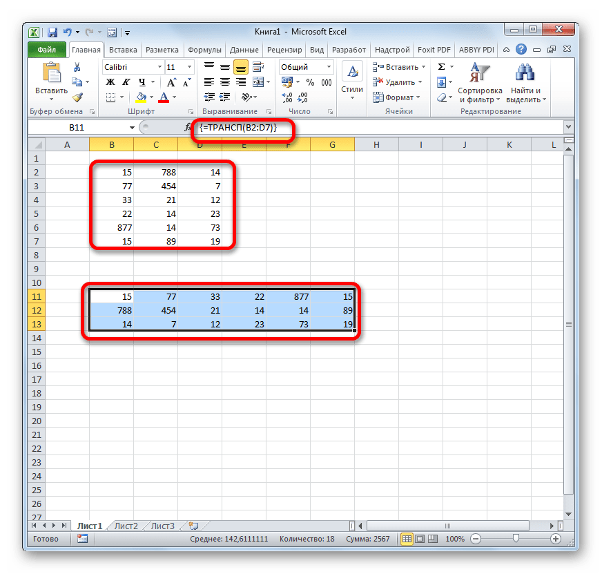
Оператор ТРАНСП

Функция ТРАНСП является типичным оператором массивов. Она позволяет переворачивать таблицы или матрицы, то есть, менять строки и столбцы местами. При этом она использует исключительно вывод результата в диапазон ячеек, поэтому после введения данного оператора обязательно нужно применять сочетание Ctrl+Shift+Enter. Также нужно отметить, что перед введением самого выражения нужно выделить на листе область, у которой количество ячеек в столбце будет равно числу ячеек в строке исходной таблицы (матрицы) и, наоборот, количество ячеек в строке должно равняться их числу в столбце исходника. Синтаксис оператора следующий:

=ТРАНСП(массив)

Урок: Транспонирование матриц в Excel

Урок: Как перевернуть таблицу в Экселе

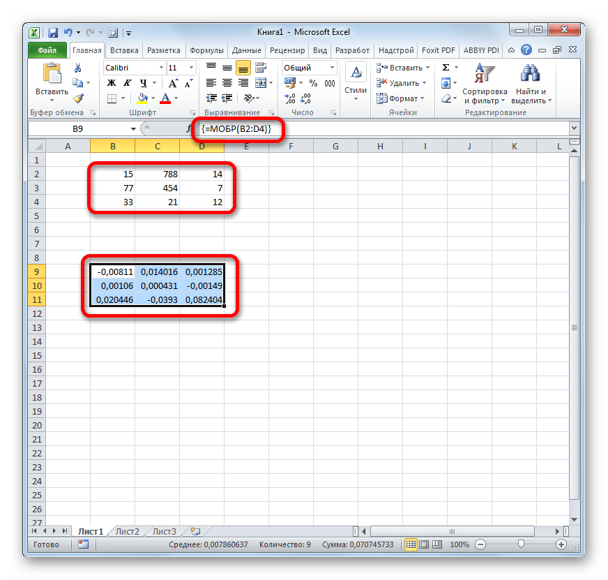
Оператор МОБР

Функция МОБР позволяет производить вычисление обратной матрицы. Все правила ввода значений у этого оператора точно такие же, как и у предыдущего. Но важно знать, что вычисление обратной матрицы возможно исключительно в том случае, если она содержит равное количество строк и столбцов, и если её определитель не равен нулю. Если применять данную функцию к области с разным количеством строк и столбцов, то вместо корректного результата на выходе отобразится значение «#ЗНАЧ!». Синтаксис у этой формулы такой:

=МОБР(массив)

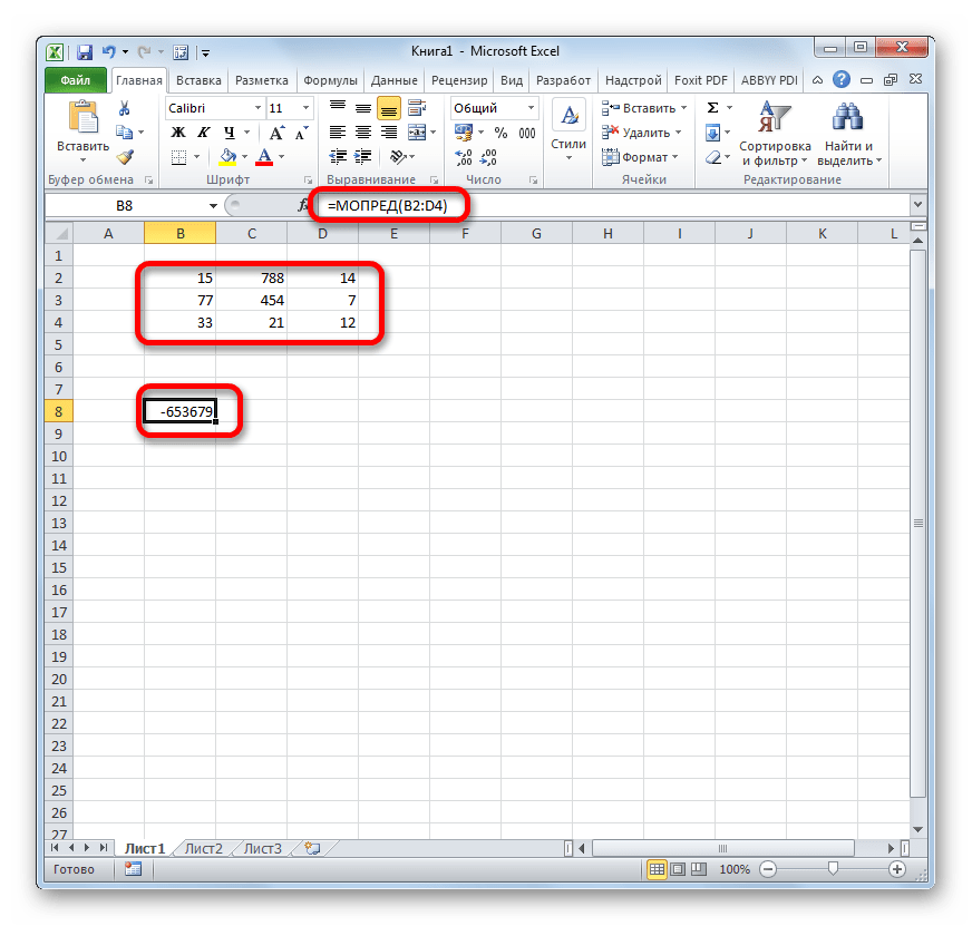
Для того чтобы рассчитать определитель, применяется функция со следующим синтаксисом:

=МОПРЕД(массив)

Урок: Обратная матрица в Excel

Как видим, операции с диапазонами помогают сэкономить время при вычислениях, а также свободное пространство листа, ведь не нужно дополнительно суммировать данные, которые объединены в диапазон, для последующей работы с ними. Все это выполняется «на лету». А для преобразования таблиц и матриц только функции массивов и подходят, так как обычные формулы не в силах справиться с подобными задачами. Но в то же время нужно учесть, что к подобным выражениям применяются дополнительные правила ввода и редактирования.