
Excel for Microsoft 365 Excel 2021 Excel 2019 Excel 2016 Excel 2013 More…Less
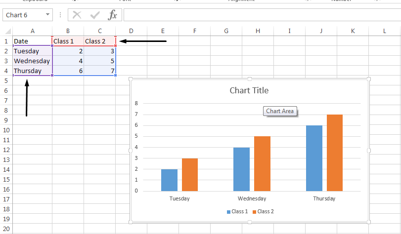
When you create a chart in Excel, it uses the information in the cell above each column or row of data as the legend name. You can change legend names by updating the information in those cells, or you can update the default legend name by using Select Data.
Note: If you create a chart without using row or column headers, Excel uses default names, starting with “Series 1.” You can learn more about how to create a chart to ensure your rows and columns are formatted properly.
In this article
-
Show the legend in your chart
-
Change the legend name in the excel data
-
Change the legend name using select data
Show the legend in your chart
-
Select the chart, click the plus sign
 in the upper-right corner of the chart, and then select the Legend check box.
 -
Optional. Click the black arrow to the right of Legend for options on where to place the legend in your chart.
 in the upper-right corner of the chart, and then select the Legend check box.
Change the legend name in the excel data
-
Select the cell in the workbook that contains the legend name you want to change.
Tip: You can first click your chart to see what cells within your data are included in your legend.
-
Type the new legend name in the selected cell, and press Enter. The legend name in the chart updates to the new legend name in your data.
-
Certain charts, such as Clustered Columns, also use the cells to the left of each row as legend names. You can edit legend names the same way.
Change the legend name using select data
-
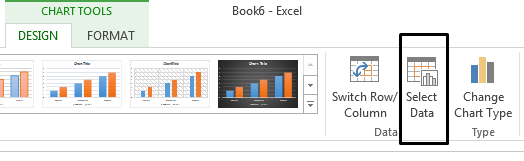
Select your chart in Excel, and click Design > Select Data.
-
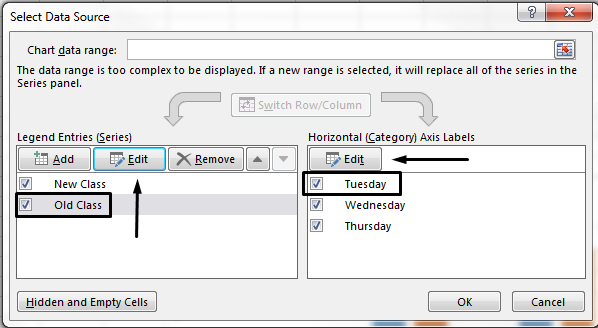
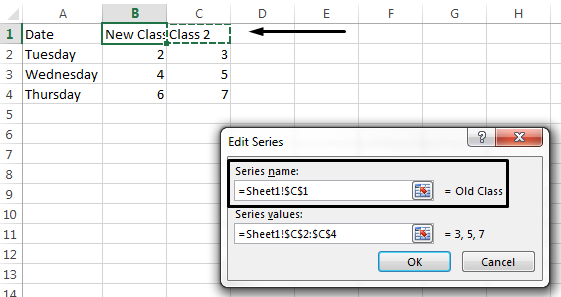
Click on the legend name you want to change in the Select Data Source dialog box, and click Edit.
Note: You can update Legend Entries and Axis Label names from this view, and multiple Edit options might be available.
-
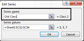
Type a legend name into the Series name text box, and click OK. The legend name in the chart changes to the new legend name.
Note: This modifies your only chart legend names, not your cell data. Alternatively, you can select a different cell in your data to use as the legend name. Click inside the Series name text box, and select the cell within your data.
Related Topics
Add or remove titles in a chart
Need more help?
Want more options?
Explore subscription benefits, browse training courses, learn how to secure your device, and more.
Communities help you ask and answer questions, give feedback, and hear from experts with rich knowledge.
This article is all about the different ways you can edit legends in Excel. Legends are indicators on a chart that show what every colorful label indicates. There is a lot you can do with legends in a chart in Microsoft Excel.
Let’s get started with this step-by-step tutorial to understand the different ways to edit legends.
You may want to learn how to create a Bar Chart or Line Chart before proceeding with this tutorial.
1. Hide or unhide legends
Here is how you can hide or unhide legends on a chart.
- Click anywhere on the chart area.
- Click on the Chart Elements icon as a green plus.
- Check Legends to unhide them and uncheck to hide them.

2. Deleting legends in a chart

- Right-click on the chart.
- Click on Select Data.
- On the left side, under Legend Entries, click Remove.
Another way to delete or remove a legend is as follows.
- Double-click the legend you want to delete.
- Right-click on it.
- Press Delete to delete only the legend.
- Press Delete Series to delete both the legend and the series.

3. Changing legend positions on Excel charts
To change the position of legends on the chart, follow these steps.
- Pull on the black arrow to set the position of legends on the chart.

- Click on More Options for more position settings for your legends in the right window pane called Format Legends.

Another way you can change the positions of legends can be as follows.
- Click anywhere on the chart.
- Go to the Design tab.
- Under Chart Layouts, pull down on Add Chart Elements.
- Pull Legends and choose your favorite position.

4. Editing or changing legend names
There are multiple ways to change the name of your legends, here is how you can do it.

- Right-click on the chart.
- Click on Select Data.
- Look on the left side under Legend Entries.
- Select the legend name you want to change.
- Click on Edit.
- Enter a new name for that legend under Series Name.

Another way you can edit the legend names can be as follows.
- Click on the chart.
- Go to the Design tab.
- Click on Select Data.
Now, edit the names of each legend as mentioned in the steps above.
5. Customizing font styles for legends
To change the font styles of your legend texts, follow these steps.

- Right-click on the legend text.
- Select Font.
- Select a custom font under Latin Text Font.
- Choose a font style like bold, italics, or regular or more under Font Style.
- Set a custom size of the text under Size.

- Set a custom font color under Font Color.
- You even have a variety of underline styles to choose from under Underline Styles.
- Once you have chosen an underline style, you can also choose the color of your underline, if you like.

- You can also add some effects to your legends like strikethrough, double strikethrough, subscript or superscript, all caps, etc. in this window.

- Under the Character Spacing tab, you can increase or decrease the spacing between legend text characters.
- You can set the points for spacing between the characters.
- Choose Normal if you don’t want any spacing.
- Choose Expanded if you want to increase spacing.
- Choose Condensed if you want to reduce spacing.
- Press OK, when you’re done.

6. Formatting legend text
You can even format the legend texts in terms of alignment, angles, or direction. Here are the steps to format legends.

- Double-click on the legend texts.
- A window on right opens named Format Legend.
- Click on Text Options besides Legend Options.
- Click on the third icon named Textbox.
- Select your desired text direction underText Direction.

- Or you can set custom text angle under Custom Angle.
Also Read: How to Indent Text in Excel?
8. Customizing legend text
You customize your legend text by applying effects to it as follows.

- Double-click on the legend texts.
- Format Legend window opens on the right
- Click on Text Options besides Legend Options.
- Click on the second icon named Text Effects.
- Select shadow effects under the Shadow tab.
- Select text reflection under the Reflection tab.
- Select glow effects under the Glow tab.
9. Text Fill & Text Outlines
You can give custom fills and outlines to legend texts in Excel. Here are the steps to give custom fills and outlines to texts.
- Double-click on the legend texts.
- Format Legend window opens on the right
- Click on Text Options besides Legend Options.
- Click on the first icon named Text Fill & Outline.

- You give custom fills to your text such as color, gradient, picture, or pattern fills under Text Fill.
- Apply custom outlines to your text under Text Outline.
Conclusion
This article was a complete detailed guide on editing legends in Microsoft Excel. Follow these steps carefully to be able to hide, unhide, customize fonts and texts, or format legend texts, and more in Excel. If you have any doubts comment your thoughts below and we will be happy to answer your queries!
References: Excelchat
- Select your chart in Excel, and click Design > Select Data.
- Click on the legend name you want to change in the Select Data Source dialog box, and click Edit.
- Type a legend name into the Series name text box, and click OK.
Contents
- 1 How do you edit Data labels in Excel?
- 2 Can you change order of legend in Excel?
- 3 How do I change the series name in Excel charts?
- 4 How do you change the legend in Excel on a Mac?
- 5 How do I change the legend color in Excel?
- 6 How do I change axis labels in Excel?
- 7 How do you add a legend in Excel?
- 8 What is legend in Excel?
- 9 How do I invert the Y axis in Excel?
- 10 How do I move the Y axis in Excel?
- 11 How do you move the legend in Excel?
- 12 How do you show the legend value in Excel pie chart?
- 13 How do I add a legend in Excel without charts?
- 14 How do you change the color of a legend in sheets?
- 15 How do I change horizontal axis labels in Excel 2020?
- 16 Where is the legend in Excel?
- 17 How can you change a legend data entry?
- 18 How do you remove a legend label without deleting the data series?
- 19 What is the difference between a legend and a key?
- 20 What is Invert Y axis?
How do you edit Data labels in Excel?
Edit the contents of a title or data label that is linked to data on the worksheet
- In the worksheet, click the cell that contains the title or data label text that you want to change.
- Edit the existing contents, or type the new text or value, and then press ENTER. The changes you made automatically appear on the chart.
Can you change order of legend in Excel?
Under Chart Tools, on the Design tab, in the Data group, click Select Data. In the Select Data Source dialog box, in the Legend Entries (Series) box, click the data series that you want to change the order of. Click the Move Up or Move Down arrows to move the data series to the position that you want.
How do I change the series name in Excel charts?
Rename a data series
- Right-click the chart with the data series you want to rename, and click Select Data.
- In the Select Data Source dialog box, under Legend Entries (Series), select the data series, and click Edit.
- In the Series name box, type the name you want to use.
How do you change the legend in Excel on a Mac?
Click the “Charts” tab on the ribbon, click “Chart Layout,” click the “Legend” button, and then click “Legend Options” to load a list of customizable options for your legend. Click the “Font” tab to customize the font. Click the “Placement” tab to change where the legend appears on the chart.
How do I change the legend color in Excel?
If you’d like to change your legend’s border color to make it more noticeable, click the Format Legend’s “Border” button and then click “Color” to display a list of colors. Click a color to apply it to the legend’s border. If nothing happens when you click a color, click the “Solid Line” radio button to select it.
How do I change axis labels in Excel?
Right-click the category labels you want to change, and click Select Data.
- In the Horizontal (Category) Axis Labels box, click Edit.
- In the Axis label range box, enter the labels you want to use, separated by commas.
How do you add a legend in Excel?
Click the chart, and then click the Chart Design tab. Click Add Chart Element > Legend. To change the position of the legend, choose Right, Top, Left, or Bottom. To change the format of the legend, click More Legend Options, and then make the format changes that you want.
What is legend in Excel?
Legend is the space located on the plotted area of the chart in excel. It has Legend keys that are connected to the data source. Legend will appear automatically when we insert a chart in excel.
How do I invert the Y axis in Excel?
To make this change, right-click and open up axis options in the Format Task pane. There, near the bottom, you’ll see a checkbox called “values in reverse order”. When I check the box, Excel reverses the plot order. Notice it also moves the horizontal axis to the right.
How do I move the Y axis in Excel?
Move Y axis to left/right/middle
- Double click at the X axis (horizontal axis) to display the Format Axis pane.
- If you are in Excel 2010 or 2007, it will open the Format Axis dialog.
- Then if you want to move the Y axis to the left, check Automatic in the Vertical axis crosses section.
How do you move the legend in Excel?
You can move the legend to any position within your chart. To move a chart’s legend, simply click on it once to select it. (You will know it is selected when handles appear around the perimeter of the legend.) Then use the mouse to click within the legend and drag the legend to the desired position on the chart.
How do you show the legend value in Excel pie chart?
To display percentage values in the legend of a pie chart
- On the design surface, right-click on the pie chart and select Series Properties. The Series Properties dialog box displays.
- In Legend, type #PERCENT for the Custom legend text property.
How do I add a legend in Excel without charts?
Hiding the legend from Chart 1 is simple and can be accomplished as follows:
- Single click on the chart.
- Select Chart | Chart Options. Excel displays the Chart Options dialog box.
- Click on the Legends tab.
- Clear the Show Legend check box.
- Click OK.
How do you change the color of a legend in sheets?
- On your computer, open a spreadsheet in Google Sheets.
- Double-click the chart you want to change.
- At the right, click Customize. Legend.
- To customize your legend, you can change the position, font, style, and color.
How do I change horizontal axis labels in Excel 2020?
Right-click the category labels to change, and click Select Data. In Horizontal (Category) Axis Labels, click Edit. In Axis label range, enter the labels you want to use, separated by commas.
Where is the legend in Excel?
In a chart or graph in a spreadsheet program such as Microsoft Excel, the legend is often located on the right-hand side of the chart or graph and is sometimes surrounded by a border. The legend is linked to the data being graphically displayed in the plot area of the chart.
How can you change a legend data entry?
Edit legend entries in the Select Data Source dialog box
On the Design tab, in the Data group, click Select Data. In the Select Data Source dialog box, in the Legend Entries (Series) box, select the legend entry that you want to change. Click Edit.
How do you remove a legend label without deleting the data series?
Replies (1) In Excel 2016 it is same, but you need to click twice. – Then click on the specific legend which you want to remove. – And then press DELETE.
What is the difference between a legend and a key?
A legend is a caption, a title or brief explanation appended to an article, illustration, cartoon, or poster. A key is an explanatory list of symbols used in a map, table, etc.
What is Invert Y axis?
A significant minority of players start every new game they play by going into the options and selecting “Invert Y axis”, which means when they push up on the stick, their onscreen avatar looks or moves downwards.
The key to understanding charts is through the use of legends. Legends are automatically created everytime we create a graph or plot our data.
 Figure 1. Final result: How to edit legend
In the chart above, the legend is located in the top center of the graph, showing a bulleted list with text “A” and “B Sales”.
When we encounter an Excel chart without a legend, we can easily add a legend through these steps:
Add legend to an Excel chart
Step 1. Click anywhere on the chart
Step 2. Click the Layout tab, then Legend
Step 3. From the Legend drop-down menu, select the position we prefer for the legend
Example: Select Show Legend at Right
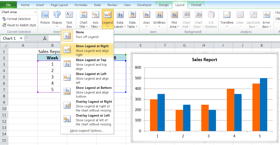 Figure 2. Adding a legend
The legend will then appear in the right side of the graph.
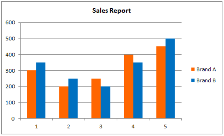 Figure 3. Output: Add legend to a chart
The legend in a chart can be edited by changing the name, or customizing its position and format.
How to change legend name?
There are two ways to change the legend name:
- Change series name in Select Data
- Change legend name
Change Series Name in Select Data
Step 1. Right-click anywhere on the chart and click Select Data
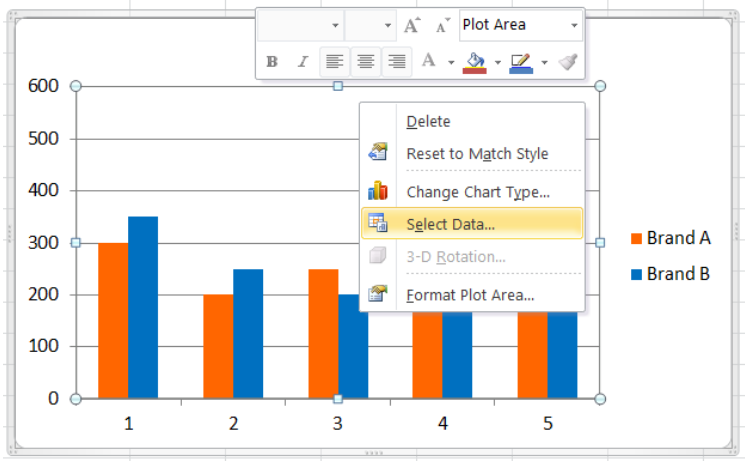 Figure 4. Change legend text through Select Data
Step 2. Select the series Brand A and click Edit
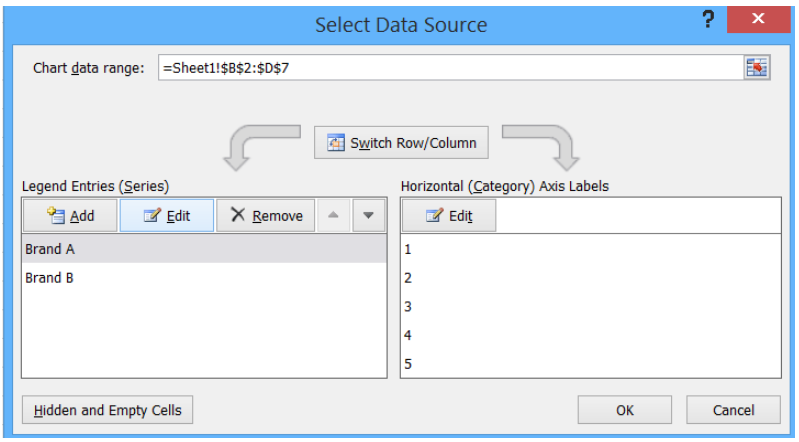 Figure 5. Edit Series in Excel
The Edit Series dialog box will pop-up.
 Figure 6. Edit Series preview pane
Step 3. Delete the current entry “=Sheet1!$C$2” in series name and enter “A” into the text box.
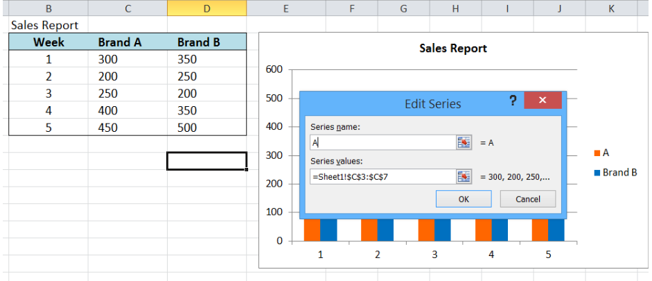 Figure 7. Changing legend text
The legend name is immediately changed to “A”.
 Figure 8. Output: How to rename legend
Change legend name
Step 1. First, we must determine the cell that contains the legend name for our chart by clicking the chart. As shown below, the column chart for Brand B is linked to cells D2:D7.
 Figure 9. Change legend text
Step 2. Since D2 contains the legend name, we select D2 and type the new legend name “B Sales”.
 Figure 10. Change legend name
As shown above, the legend name on the chart is instantly updated from “Brand B” to “B Sales”.
How to edit legend?
Legends can be customized by changing the layout, position or format.
How to change legend position?
It is very easy to change the legend position in Excel. Simply click the chart, then click the Layout tab. Under Legend, choose the preferred position from the drop-down menu.
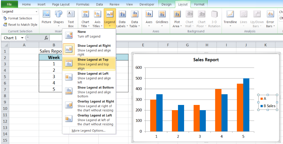 Figure 11. Change legend position
Example:
Select Show Legend at Top from the drop-down menu. As shown below, the legend is transferred to the top of the chart.
 Figure 12. Output: Change legend position
How to edit legend format?
In order to change the format, right-click the legend and select Format Legend.
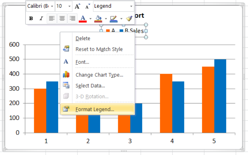 Figure 13. Edit legend through Format Legend
The Format Legend dialog box will appear. There are several options where we can change the legend position, fill, border color, border styles, and other formatting options.
 Figure 14. Format legend preview pane
Example:
We want to fill the legend box with Aqua, Accent 5, Lighter 60%.
We click Fill, then tick Solid Fill.
 Figure 15. Change legend fill
Choose the color we prefer and click OK. The fill color will automatically be updated to the chosen color.
 Figure 16. Select fill color for legend
We can add more formatting changes. Below chart shows the legend format with a 5% pattern fill and an orange border color.
 Figure 17. Final result: How to edit legend
Instant Connection to an Expert through our Excelchat Service
Most of the time, the problem you will need to solve will be more complex than a simple application of a formula or function. If you want to save hours of research and frustration, try our live Excelchat service! Our Excel Experts are available 24/7 to answer any Excel question you may have. We guarantee a connection within 30 seconds and a customized solution within 20 minutes.
eight simple ways to edit a legend in Excel
One essential element of our charts and graphs rarely gets the attention it deserves: the legend.
Without a clear and thoughtfully-incorporated legend, viewers of our data communications will struggle to understand exactly what we’re presenting to them. Any additional effort an audience needs to devote to solving the mystery of “which data series is green?” or “what’s the difference between square data markers and circles?” is energy they won’t have to put towards grasping your visual’s important insights. A well-designed legend will remove that cognitive burden.
With every graph you create, plan to spend some time crafting a legend that supports and clarifies the data you’re presenting.
Almost every chart template in Excel will place a legend into a new graph by default. For bar charts, it’s usually set off to the right:

Did you know, however, that you can edit your legends? In fact, there are many things that you can do directly in Excel (or directly in PowerPoint) to customize this essential element of your communication.
But first, here are a couple of things you CAN’T do to your legend in Excel.
-
Reorder the elements in your legend. In some visualization tools, you can drag entries in the legend to change the way the series are sorted, but in Excel the order is determined in the data source itself by the series order.
-
Modify the text of the entries. Unlike data labels, into which you can re-type or add new text, legend entries are also fully determined by the data source. If you wanted this graph’s legend to be Title Case or ALL CAPS, you’d have to change that in the underlying worksheet.
Here are eight simple ways to customize your Excel legend.
1. Place it somewhere else.
As long as you haven’t resized your graph’s plot area (the space reserved for the data itself), you can use the “Format Legend” pane in Excel to move your legend to the top, left, bottom, or top right corner of your chart area. When you do this, your plot area will resize to make room for the relocated legend.

In this graph, the legend position is set to «Top» rather than «Right.» Notice that the plot area automatically gets shorter and wider to make room for the legend.
How to do it in Excel:
Click on your chart, and then click the “Format” tab in your Excel ribbon at the top of the window. From the very right of the ribbon, click “Format Pane.” Once that pane is open, click on the legend itself within your chart. In your Format Pane, the options will then look something like this:
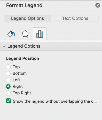
Then, set that legend position to be whichever location you want. My tendency is to put the legend at the top, because of people’s tendency to scan any new visual from top-to-bottom; that way, a reader will know what dataset corresponds to each color or marker type before they start to evaluate the information in the graph.
2. Overlay the legend atop your data.
Excel prefers not to have the legend and the plot area use the same physical space…but if you want them to overlap each other, you can make that happen.
How to do it in Excel:
That bottom option in the Format Legend pane above—the one that reads “Show the legend without overlapping the c…”—is the key item here.
If that box is checked, the legend will not overlap the plot area at all. By unchecking it, the legend will then float on top of the plot area (and any data series that happen to be there).
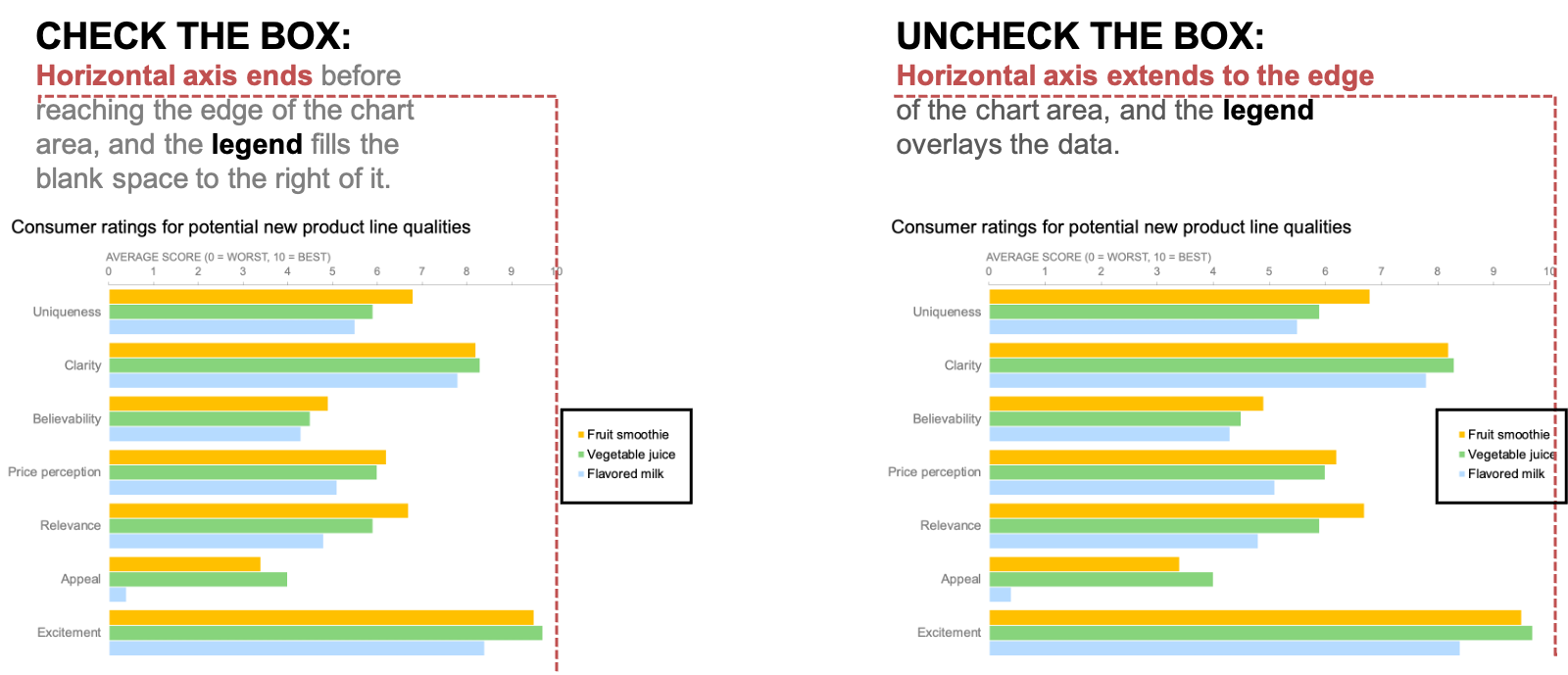
By default, the available plot area for a graph stops short of the space that Excel reserves for the legend. Unchecking one box in the “Format Legend” pane will extend your graph’s plot area all the way to the edge of your available space, and will place the legend such that it overlaps with the visual.
3. Hand-drag it to a precise location of your choice.
You’re not limited just to the options Excel’s Format Pane provides by default. You can actually put your legend anywhere you want in your chart area. For instance, I put mine slightly closer to the bars in this example:

For this view, I hand-dragged the legend as far to the left, within the available plot area, as I could without it overlapping actual data bars or feeling too crowded.
How to do it in Excel:
If you click on your legend, you’ll see it highlighted with squares at each corner and at the midpoint of each line.

Clicking on the legend directly will select it, and make these little squares (called “handles”) visible.
Once the legend is highlighted like this, click and hold your cursor down in the middle of the outlined legend (make sure your cursor looks like a plus sign with arrows on the ends—that means you’ll be able to move the legend without distorting it). Then, drag-and-drop it anywhere you want in your chart area.
4. If, for some reason, you insist on doing so: add outlines, shading, or other visual effects.
99 times out of 100, you won’t need to do this. Decorative effects such as these primarily serve only to clutter up a visual. However, since it’s impossible to predict every possible scenario in which you’ll be creating a chart, there may be a time when you’ll want to visually set off your legend from surrounding elements. In that unlikely event, it’s worth knowing that Excel offers you the ability to add fills, borders, and more to your legend.
I made mine super pretty! Look at my beautiful shaded, outlined, and glowing legend:

Just because you can put a gray background, a thick dotted border, and a purple glow around your legend, doesn’t mean you should. In fact, you probably shouldn’t…but it’s important to know how to make these kinds of changes on the VERY rare occasion that it becomes necessary to do so.
How to do it in Excel:
To reiterate: I am not encouraging you to bling out your legends on a regular basis. But if for some reason you find it’s necessary to do so…you can click on the legend in your graph, and then change the Fill, Stroke, and other options from the Format Pane:
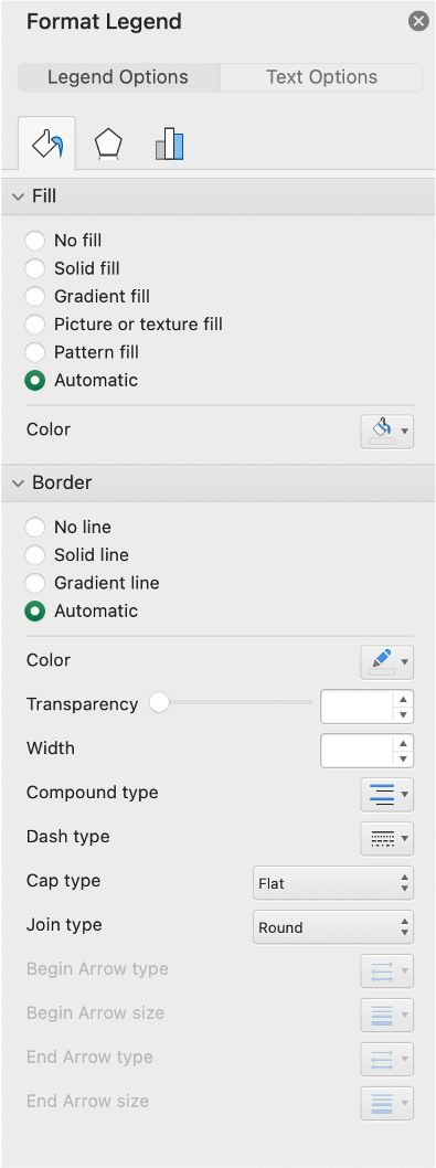
From the “Format Legend” pane, you can change the fill, border, and other appearance traits of your legend.
Please apply this knowledge with the utmost restraint. With great power comes great responsibility.
5. Resize the dimensions of the legend and the text inside it.
You can make your legend taller, wider or both. At the same time, you can increase or decrease the font size for your legend without changing the font size of the rest of the graph.

This legend is manually resized to be taller.

This legend’s font size has been increased.
How to do it in Excel:
To resize the dimensions of the legend, highlight it so that you get this outline again:
Then, click on any one of the squares (they’re called “handles”) to make the legend larger in that direction. The corner handles let you change width and height at the same time; the handles in the middle of straight lines only let you change one or the other.
Resizing the fonts in the legend is pretty straightforward: you click on your legend, then click the “Home” tab in your Excel ribbon, and change the font size, family, weight, or anything else you want just the way you’d change any other text.
6. Use the legend to change the look of a data series.
It’s not surprising that when you change the color of a data series in your chart, your legend updates to show the correct new color. What’s less well-known is that you can do this operation in reverse as well. For instance, I used the legend to reset my “Fruit smoothie” color to red.

You can use the legend itself to change the color of any or all data series in your view.
How to do it in Excel:
Click once on the legend (to get the “handles” to show up around the whole thing), and then click a second time on one specific item in the legend itself. I clicked on “Fruit smoothie,” and it looked like this:

Click on the legend once, and then again on a specific entry, to select just one part of the legend (and its related data series.)
Then, I changed the fill color of that item to red in the Format Pane, which had changed to show the header “Format Legend Entry:”

The “Format Legend Entry” pane will appear if you only select a single element within your legend.
That’s a handy thing to remember: “Format Legend” refers to everything in the entire legend, but “Format Legend Entry” refers only to the item in the legend that describes a particular data series.
7. Remove unwanted legend entries.
This would be favorable when you’re doing some creative Excel brute-forcing—perhaps there are some series you need on the back end but don’t want displayed in the legend itself. You can actively delete entries from your legend directly, without removing the data from the chart itself. As you can see here, “Flavored milk” is gone from the legend, but the data still persists in the view.

Even though “Flavored milk” has been removed from the legend, the data series it referred to is still present in the view.
How to do it in Excel:
Click once in the legend and then click a second time on the specific legend entry you’d like to remove, and then just press the “Delete” key.
8. Remove the legend entirely, and do it yourself!
This, of all the techniques we’ve covered here, is my preferred option. Although you can use Excel settings and menus to create quick-and-dirty legends, and even customize them somewhat, your communications will benefit from a bit more thoughtfulness and polish. Either delete or hide the Excel legend, and instead add some text in useful places.
You could incorporate your legend as a subheader, so your readers see it right away and know which data series goes with which color.

Using appropriately colored text as a subheader can be an elegant approach to incoporating a legend into the graph view.
How to do it in Excel:
Click on your graph, and then in your Excel ribbon, select the “Format” tab next to the “Chart Design” tab. Towards the left hand side of your ribbon, click on the icon of a text box. That will place a blank text box in your Chart Area, which you can move, edit, and format just like a regular text box.

Type out the names of your data series, format them as you see fit, and place the subheader you’ve created just below the title of your graph.
Or, you could directly label the first instance of each of your data series, either at the ends of the bars or inside the base of them:

Label the first instance of each series at the ends…

…or at the bases of the bars as another legend option.
How to do it in Excel:
You can use the same technique for this as for adding a subheader, or you could use Excel’s ability to add data labels by interacting with the bars themselves. Either of these approaches also would work for line graphs, or most any other chart type you’d use on a regular basis.
Whichever approach you choose, let your decision be based on what will best serve your audience, rather than on what your graphing tool offers you as a default setting.
More Excel how-to’s:
-
For better bar charts, adjust the gap width
-
To emphasize a specific point, add data labels
-
To depict a range of values, add a shaded band
-
To create a frame of reference, embed a vertical line
-
To show a distribution of data, create a dotplot
-
For cleaner alignment, put graph elements directly in cells
-
To have more control over data label formatting, embed labels into your graphs
-
To make a stellar line graph, add thoughtful design elements (available to premium subscribers)