17 авг. 2022 г.
читать 2 мин
В этом руководстве объясняется, как преобразовать дату в число в трех различных сценариях:
1. Преобразуйте одну дату в число
2. Преобразуйте несколько дат в числа
3. Преобразование даты в количество дней с другой даты
Давайте прыгать!
Пример 1: преобразование одной даты в число
Предположим, мы хотим преобразовать дату «10.02.2022» в число в Excel.
Для этого мы можем использовать функцию ДАТАЗНАЧ в Excel:
=DATEVALUE("2/10/2022")
По умолчанию эта функция вычисляет количество дней между заданной датой и 01.01.1900 .
На следующем снимке экрана показано, как использовать эту функцию на практике:
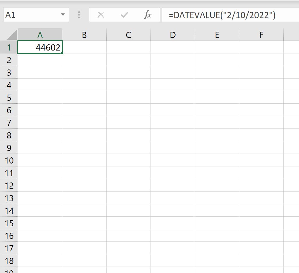
Это говорит нам о том, что между 10.02.2022 и 01.01.1900 существует разница в 44 602 дня.
Пример 2. Преобразование нескольких дат в числа
Предположим, у нас есть следующий список дат в Excel:

Чтобы преобразовать каждую из этих дат в число, мы можем выделить диапазон ячеек, содержащих даты, затем щелкнуть раскрывающееся меню «Числовой формат » на вкладке « Главная » и выбрать « Число »:

Это автоматически преобразует каждую дату в число, представляющее количество дней между каждой датой и 01.01.1900 :

Пример 3. Преобразование даты в количество дней, прошедших с другой даты
Мы можем использовать следующую формулу для преобразования даты в количество дней, прошедших с другой даты:
=DATEDIF( B2 , A2 , "d")
Эта конкретная формула вычисляет количество дней между датой в ячейке B2 и датой в ячейке A2 .
На следующем снимке экрана показано, как использовать формулу DATEDIF для расчета количества дней между датами в столбце A и 01.01.2022:

Вот как интерпретировать значения в столбце B:
- Между 01.01.2022 и 01.04.2022 есть 3 дня.
- Между 01.01.2022 и 01.01.2022 8 дней.
- Между 01.01.2022 и 15.01.2022 14 дней.
И так далее.
Дополнительные ресурсы
В следующих руководствах объясняется, как выполнять другие распространенные задачи в Excel:
Как автозаполнять даты в Excel
Как использовать СЧЁТЕСЛИМН с диапазоном дат в Excel
Как рассчитать среднее значение между двумя датами в Excel
This tutorial explains how to convert a date to a number in three different scenarios:
1. Convert One Date to Number
2. Convert Several Dates to Numbers
3. Convert Date to Number of Days Since Another Date
Let’s jump in!
Example 1: Convert One Date to Number
Suppose we would like to convert the date “2/10/2022” to a number in Excel.
We can use the DATEVALUE function in Excel to do so:
=DATEVALUE("2/10/2022")
By default, this function calculates the number of days between a given date and 1/1/1900.
The following screenshot shows how to use this function in practice:

This tells us that there is a difference of 44,602 days between 2/10/2022 and 1/1/1900.
Example 2: Convert Several Dates to Numbers
Suppose we have the following list of dates in Excel:

To convert each of these dates to a number, we can highlight the range of cells that contain the dates, then click the Number format dropdown menu on the Home tab and choose Number:

This will automatically convert each date to a number that represents the number of days between each date and 1/1/1900:

Example 3: Convert Date to Number of Days Since Another Date
We can use the following formula to convert a date to a number of days since another date:
=DATEDIF(B2, A2, "d")
This particular formula calculates the number of days between the date in cell B2 and the date in cell A2.
The following screenshot shows how to use the DATEDIF formula to calculate the number of days between the dates in column A and 1/1/2022:

Here’s how to interpret the values in column B:
- There are 3 days between 1/1/2022 and 1/4/2022.
- There are 8 days between 1/1/2022 and 1/9/2022.
- There are 14 days between 1/1/2022 and 1/15/2022.
And so on.
Additional Resources
The following tutorials explain how to perform other common tasks in Excel:
How to AutoFill Dates in Excel
How to Use COUNTIFS with a Date Range in Excel
How to Calculate Average If Between Two Dates in Excel
Excel for Microsoft 365 Excel 2021 Excel 2019 Excel 2016 Excel 2013 Excel 2010 More…Less
Dates are often a critical part of data analysis. You often ask questions such as: when was a product purchased, how long will a task in a project take, or what is the average revenue for a fiscal quarter? Entering dates correctly is essential to ensuring accurate results. But formatting dates so that they are easy to understand is equally important to ensuring correct interpretation of those results.
Important: Because the rules that govern the way that any calculation program interprets dates are complex, you should be as specific as possible about dates whenever you enter them. This will produce the highest level of accuracy in your date calculations.
Excel stores dates as sequential numbers that are called serial values. For example, in Excel for Windows, January 1, 1900 is serial number 1, and January 1, 2008 is serial number 39448 because it is 39,448 days after January 1, 1900.
Excel stores times as decimal fractions because time is considered a portion of a day. The decimal number is a value ranging from 0 (zero) to 0.99999999, representing the times from 0:00:00 (12:00:00 A.M.) to 23:59:59 (11:59:59 P.M.).
Because dates and times are values, they can be added, subtracted, and included in other calculations. You can view a date as a serial value and a time as a decimal fraction by changing the format of the cell that contains the date or time to General format.
Both Excel for Mac and Excel for Windows support the 1900 and 1904 date systems. The default date system for Excel for Windows is 1900; and the default date system for Excel for Mac is 1904.
Originally, Excel for Windows was based on the 1900 date system, because it enabled better compatibility with other spreadsheet programs that were designed to run under MS-DOS and Microsoft Windows, and therefore it became the default date system. Originally, Excel for Mac was based on the 1904 date system, because it enabled better compatibility with early Macintosh computers that did not support dates before January 2, 1904, and therefore it became the default date system.
The following table shows the first date and the last date for each date system and the serial value associated with each date.
|
Date system |
First date |
Last date |
|---|---|---|
|
1900 |
January 1, 1900 |
December 31, 9999 |
|
1904 |
January 2, 1904 |
December 31, 9999 |
Because the two date systems use different starting days, the same date is represented by different serial values in each date system. For example, July 5, 2007 can have two different serial values, depending on the date system that is used.
|
Date system |
Serial value of July 5, 2007 |
|---|---|
|
1900 |
37806 |
|
1904 |
39268 |
The difference between the two date systems is 1,462 days; that is, the serial value of a date in the 1900 date system is always 1,462 days greater than the serial value of the same date in the 1904 date system. Conversely, the serial value of a date in the 1904 date system is always 1,462 days less than the serial value of the same date in the 1900 date system. 1,462 days is equal to four years and one day (which includes one leap day).
Important: To ensure that year values are interpreted as you intended, type year values as four digits (for example, 2001, not 01). By entering four-digit years, Excel won’t interpret the century for you.
If you enter a date with a two-digit year in a text formatted cell or as a text argument in a function, such as =YEAR(«1/1/31»), Excel interprets the year as follows:
-
00 through 29 is interpreted as the years 2000 through 2029. For example, if you type the date 5/28/19, Excel assumes the date is May 28, 2019.
-
30 through 99 is interpreted as the years 1930 through 1999. For example, if you type the date 5/28/98, Excel assumes the date is May 28, 1998.
In Microsoft Windows, you can change the way two-digit years are interpreted for all Windows programs that you have installed.
Windows 10
-
In the search box on the taskbar, type control panel, and then select Control Panel.
-
Under Clock, Language and Region, click Change date, time, or number formats
-
Click Regional and Language Options.
-
In the Region dialog box, click Additional settings.
-
Click the Date tab.
-
In the When a two-digit year is entered, interpret it as a year between box, change the upper limit for the century.
As you change the upper-limit year, the lower-limit year automatically changes.
-
Click OK.
Windows 8
-
Swipe in from the right edge of the screen, tap Search (or if you’re using a mouse, point to the upper-right corner of the screen, move the mouse pointer down, and then click Search), enter Control Panel in the search box, and then tap or click Control Panel.
-
Under Clock, Language and Region, click Change date, time, or number formats.
-
In the Region dialog box, click Additional settings.
-
Click the Date tab.
-
In the When a two-digit year is entered, interpret it as a year between box, change the upper limit for the century.
As you change the upper-limit year, the lower-limit year automatically changes.
-
Click OK.
Windows 7
-
Click the Start button, and then click Control Panel.
-
Click Region and Language.
-
In the Region dialog box, click Additional settings.
-
Click the Date tab.
-
In the When a two-digit year is entered, interpret it as a year between box, change the upper limit for the century.
As you change the upper-limit year, the lower-limit year automatically changes.
-
Click OK.
By default, as you enter dates in a workbook, the dates are formatted to display two-digit years. When you change the default date format to a different format by using this procedure, the display of dates that were previously entered in your workbook will change to the new format as long as the dates haven’t been formatted by using the Format Cells dialog box (On the Home tab, in the Number group, click the Dialog Box Launcher).
Windows 10
-
In the search box on the taskbar, type control panel, and then select Control Panel.
-
Under Clock, Language and Region, click Change date, time, or number formats
-
Click Regional and Language Options.
-
In the Region dialog box, click Additional settings.
-
Click the Date tab.
-
In the Short date format list, click a format that uses four digits for the year («yyyy»).
-
Click OK.
Windows 8
-
Swipe in from the right edge of the screen, tap Search (or if you’re using a mouse, point to the upper-right corner of the screen, move the mouse pointer down, and then click Search), enter Control Panel in the search box, and then tap or click Control Panel.
-
Under Clock, Language and Region, click Change date, time, or number formats.
-
In the Region dialog box, click Additional settings.
-
Click the Date tab.
-
In the Short date format list, click a format that uses four digits for the year («yyyy»).
-
Click OK.
Windows 7
-
Click the Start button, and then click Control Panel.
-
Click Region and Language.
-
In the Region dialog box, click Additional settings.
-
Click the Date tab.
-
In the Short date format list, click a format that uses four digits for the year («yyyy»).
-
Click OK.
The date system changes automatically when you open a document from another platform. For example, if you are working in Excel and you open a document that was created in Excel for Mac, the 1904 date system check box is selected automatically.
You can change the date system by doing the following:
-
Click File > Options > Advanced.
-
Under the When calculating this workbook section, select the workbook that you want, and then select or clear the Use 1904 date system check box.
You can encounter problems when you copy and paste dates or when you create external references between workbooks based on the two different date systems. Dates can appear four years and one day earlier or later than the date that you expect. You can encounter these problems whether you are using Excel for Windows, Excel for Mac, or both.
For example, if you copy the date July 5, 2007 from a workbook that uses the 1900 date system and then paste the date into a workbook that uses the 1904 date system, the date appears as July 6, 2011, which is 1,462 days later. Alternatively, if you copy the date July 5, 2007 from a workbook that uses the 1904 date system and then paste the date into a workbook that uses the 1900 date system, the date appears as July 4, 2003, which is 1,462 days earlier. For background information, see Date systems in Excel.
Correct a copy and paste problem
-
In an empty cell, enter the value 1462.
-
Select that cell, and then on the Home tab, in the Clipboard group, click Copy.
-
Select all of the cells that contain the incorrect dates.
-
On the Home tab, in the Clipboard group, click Paste, and then click Paste Special.

-
In the Paste Special dialog box, under Paste, click Values, and then under Operation, do one of the following:
-
To set the date as four years and one day later, click Add.
-
To set the date as four years and one day earlier, click Subtract.
-

Correct an external reference problem
If you are using an external reference to a date in another workbook with a different date system, you can modify the external reference by doing one of the following:
-
To set the date as four years and one day later, add 1,462 to it. For example:
=[Book2]Sheet1!$A$1+1462
-
To set the date as four years and one day earlier, subtract 1,462 from it. For example:
=[Book1]Sheet1!$A$1-1462
Need more help?
You can always ask an expert in the Excel Tech Community or get support in the Answers community.
See Also
Format a date the way you want
Display numbers as dates or times
Enter data manually in worksheet cells
Examples of commonly used formulas
Need more help?
To change the cell format from date to number we convert the formatting into General Format in Microsoft Excel.
There are three different ways to change the formatting from date to number.
1st Shortcut Key
2nd Format Cells
3rd Command Button
Let’s take an example and understand how we can convert cell formatting from date to number or general formatting.
We have date in column D. In column E we will learn to convert the cell format from date to number through shortcut key, in column F through Format Cells and in Column G through Command button.
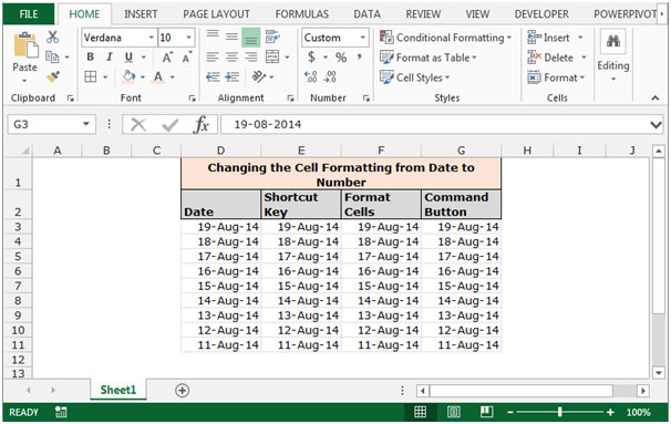
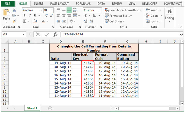
To change the cell formatting by using the Shortcut Key
Follow below given steps:-
- Select the range E3:E11.
- Press the key Ctrl+Shift+~ on your keyboard.
- Cells formatting will get convert into numbers.
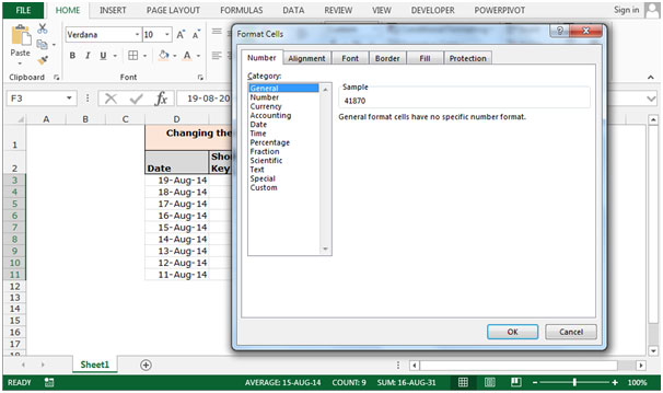
To change the cell formatting by using Format Cells
Follow below given steps:-
- Select the range F3:F11 and press the key Ctrl+1 on your keyboard.
- A format Cells dialog box will appear.
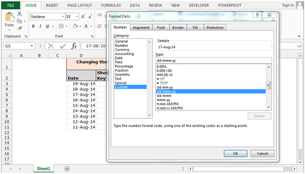
- In the Number Tab, Click on General.
- We can see the formatting in sample preview.
- The function will convert the formatting into general formatting.

To change the cell formatting by using Command Button
Follow below given steps:-
- Select the range G3:G11.
- Go to Home Tab click on General in the Number group.

- Date format will get convert in General format.
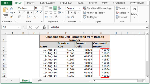
These are the ways in which we can convert the cell formatting from date to number in Microsoft Excel.
![]()
If you liked our blogs, share it with your friends on Facebook. And also you can follow us on Twitter and Facebook.
We would love to hear from you, do let us know how we can improve, complement or innovate our work and make it better for you. Write us at info@exceltip.com
Return to Excel Formulas List
Download Example Workbook
Download the example workbook
This tutorial will demonstrate how to convert a date to a serial number corresponding to that date (or vis-a-versa) in Excel and Google Sheets
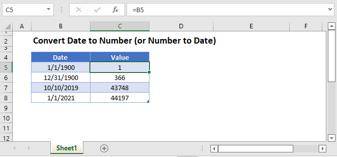
Date to Number
To convert a date to a serial number, all you need to do is change the formatting to General:
However, this won’t work if the date is stored as text.
Date Stored as Text to Number
If the date is stored as text, you can use DATEVALUE convert it to an Excel date:
=DATEVALUE(B3)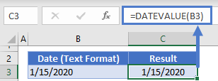
Then you can change the formatting to general to see the serial number.
Number to Date
To convert a serial number to a date, all you need to do is the change the formatting from General (or Number) to a date format (ex. Short Date):
Convert Date to Number in Google Sheets
All of the above examples work exactly the same in Google Sheets as in Excel.