Change column to number excel - Word и Excel - помощь в работе с программами

Convert numbers stored as text to numbers

Excel for Microsoft 365 Excel for Microsoft 365 for Mac Excel 2021 Excel 2021 for Mac Excel 2019 Excel 2019 for Mac Excel 2016 Excel 2016 for Mac Excel 2013 Excel Web App Excel 2010 Excel 2007 Excel for Mac 2011 Excel Starter 2010 More…Less

Numbers that are stored as text can cause unexpected results, like an uncalculated formula showing instead of a result. Most of the time, Excel will recognize this and you’ll see an alert next to the cell where numbers are being stored as text. If you see the alert, select the cells, and then click to choose a convert option.

Check out Format numbers to learn more about formatting numbers and text in Excel.

If the alert button is not available, do the following:

1. Select a column

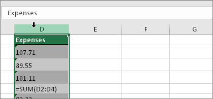
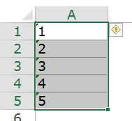
Select a column with this problem. If you don’t want to convert the whole column, you can select one or more cells instead. Just be sure the cells you select are in the same column, otherwise this process won’t work. (See «Other ways to convert» below if you have this problem in more than one column.)

2. Click this button

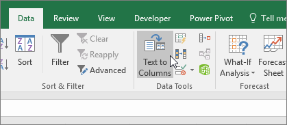
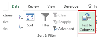
The Text to Columns button is typically used for splitting a column, but it can also be used to convert a single column of text to numbers. On the Data tab, click Text to Columns.

3. Click Apply

The rest of the Text to Columns wizard steps are best for splitting a column. Since you’re just converting text in a column, you can click Finish right away, and Excel will convert the cells.

4. Set the format

Press CTRL + 1 (or + 1 on the Mac). Then select any format.

Note: If you still see formulas that are not showing as numeric results, then you may have Show Formulas turned on. Go to the Formulas tab and make sure Show Formulas is turned off.

Other ways to convert:

You can use the VALUE function to return just the numeric value of the text.

1. Insert a new column

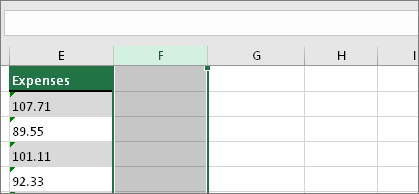
Insert a new column next to the cells with text. In this example, column E contains the text stored as numbers. Column F is the new column.

2. Use the VALUE function

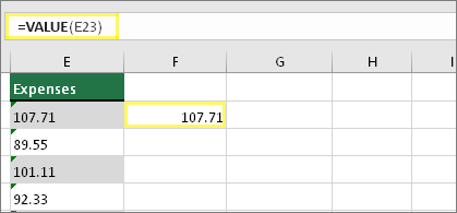
In one of the cells of the new column, type =VALUE() and inside the parentheses, type a cell reference that contains text stored as numbers. In this example it’s cell E23.

3. Rest your cursor here

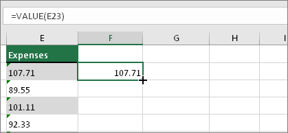
Now you’ll fill the cell’s formula down, into the other cells. If you’ve never done this before, here’s how to do it: Rest your cursor on the lower-right corner of the cell until it changes to a plus sign.

4. Click and drag down

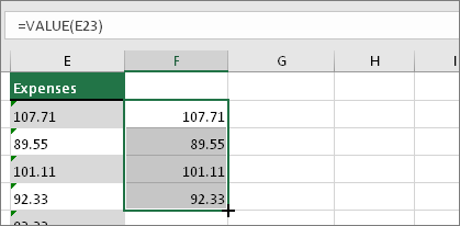
Click and drag down to fill the formula to the other cells. After that’s done, you can use this new column, or you can copy and paste these new values to the original column. Here’s how to do that: Select the cells with the new formula. Press CTRL + C. Click the first cell of the original column. Then on the Home tab, click the arrow below Paste, and then click Paste Special > Values.

If the steps above didn’t work, you can use this method, which can be used if you’re trying to convert more than one column of text.

Select a blank cell that doesn’t have this problem, type the number 1 into it, and then press Enter.
Press CTRL + C to copy the cell.
Select the cells that have numbers stored as text.
On the Home tab, click Paste > Paste Special.
Click Multiply, and then click OK. Excel multiplies each cell by 1, and in doing so, converts the text to numbers.
Press CTRL + 1 (or + 1 on the Mac). Then select any format.

How do I show column numbers in Excel?

Show column number

Click File tab > Options.
In the Excel Options dialog box, select Formulas and check R1C1 reference style.
Click OK.

How do I convert text to values in Excel?

Use the Format Cells option to convert number to text in Excel

Select the range with the numeric values you want to format as text.
Right click on them and pick the Format Cells… option from the menu list. Tip. You can display the Format Cells…
On the Format Cells window select Text under the Number tab and click OK.

How do I convert a column of numbers to column names in Excel?

To convert a column number to an Excel column letter (e.g. A, B, C, etc.) you can use a formula based on the ADDRESS and SUBSTITUTE functions. With this information, ADDRESS returns the text “A1”.

How do I change the number format in Excel?

You can use the Format Cells dialog to find the other available format codes:

Press Ctrl+1 ( +1 on the Mac) to bring up the Format Cells dialog.
Select the format you want from the Number tab.
Select the Custom option,
The format code you want is now shown in the Type box.

Why does Excel have numbers for columns?

Cause: The default cell reference style (A1), which refers to columns as letters and refers to rows as numbers, was changed. Solution: Clear the R1C1 reference style selection in Excel preferences. On the Excel menu, click Preferences.The column headings now show A, B, and C, instead of 1, 2, 3, and so on.

How do I show columns and row numbers in Excel?

On the Ribbon, click the Page Layout tab. In the Sheet Options group, under Headings, select the Print check box. , and then under Print, select the Row and column headings check box .

How do I get columns and row numbers in Excel?

It is quite easy to figure out the row number or column number if you know a cell’s address. If the cell address is NK60, it shows the row number is 60; and you can get the column with the formula of =Column(NK60). Of course you can get the row number with formula of =Row(NK60).

How do I get row numbers in Excel?

Use the ROW function to number rows

In the first cell of the range that you want to number, type =ROW(A1). The ROW function returns the number of the row that you reference. For example, =ROW(A1) returns the number 1.
Drag the fill handle. across the range that you want to fill.

How do I format numbers in Excel?

Formatting the Numbers in an Excel Text String

Right-click any cell and select Format Cell.
On the Number format tab, select the formatting you need.
Select Custom from the Category list on the left of the Number Format dialog box.
Copy the syntax found in the Type input box.

What are the different ways in formatting numbers?

How to change number formats. You can select standard number formats (General, Number, Currency, Accounting, Short Date, Long Date, Time, Percentage, Fraction, Scientific, Text) on the home tab of the ribbon using the Number Format menu. Note: As you enter data, Excel will sometimes change number formats automatically.

How do I change the column title in Excel?

Select a column, and then select Transform > Rename. You can also double-click the column header. Enter the new name.

How do I change rows and column names in Excel?

Rename columns and rows in a worksheet

Click the row or column header you want to rename.
Edit the column or row name between the last set of quotation marks. In the example above, you would overwrite the column name Gold Collection.
Press Enter. The header updates.

How do I change Excel columns from numbers to alphabets?

To change the column headings to letters, select the File tab in the toolbar at the top of the screen and then click on Options at the bottom of the menu. When the Excel Options window appears, click on the Formulas option on the left. Then uncheck the option called “R1C1 reference style” and click on the OK button.

How do I get rid of column 1 headers in Excel?

Go to Table Tools > Design on the Ribbon. In the Table Style Options group, select the Header Row check box to hide or display the table headers. If you rename the header rows and then turn off the header row, the original values you input will be retained if you turn the header row back on.

How do I change the row numbers in Excel?

Here are the steps to use Fill Series to number rows in Excel:

Enter 1 in cell A2.
Go to the Home tab.
In the Editing Group, click on the Fill drop-down.
From the drop-down, select ‘Series..’.
In the ‘Series’ dialog box, select ‘Columns’ in the ‘Series in’ options.
Specify the Stop value.
Click OK.

What is an Xlookup in Excel?

Use the XLOOKUP function to find things in a table or range by row.With XLOOKUP, you can look in one column for a search term, and return a result from the same row in another column, regardless of which side the return column is on.

Why can’t I see row numbers in Excel?

In order to show (or hide) the row and column numbers and letters go to the View ribbon. Set the check mark at “Headings”. That’s it!

How do I add a numbered list in Excel?

Click the Home tab in the Ribbon. Click the Bullets and Numbering option in the new group you created. The new group is on the far right side of the Home tab. In the Bullets and Numbering window, select the type of bulleted or numbered list you want to add to the text box and click OK.

How do I automatically number in sheets?

Use autofill to complete a series

On your computer, open a spreadsheet in Google Sheets.
In a column or row, enter text, numbers, or dates in at least two cells next to each other.
Highlight the cells. You’ll see a small blue box in the lower right corner.
Drag the blue box any number of cells down or across.

Источник

Excel COLUMN to Number (Table of Content)

Convert Column Heading to a Number
How to use the COLUMN function in Excel?
How to Change the Excel Reference Style?
What is the R1C1 Reference Style?

Excel COLUMN to Number

In Excel, column headings or labels are numbers instead of alphabets. This feature is called Excel reference style.

Convert Column Heading to a Number

Excel provides a built-in COLUMN function that falls under the Lookup/Reference function category. This function returns the column number for a given cell reference.

For Example: For finding the column number of Cell A10, we will use the formula like below:

=COLUMN (A10)

Which gives 1 as a result because column A is the first column.

Formula:

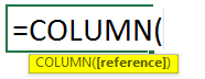
Where the passing argument reference is optional.

This function accepts only one argument, which is optional. It takes cell reference or a range of cells for which we want to find the column number. It returns the numeric value.

How to Use COLUMN Function in Excel?

Let’s take some examples to understand the usage of this function.

You can download this COLUMN to Number Excel Template here – COLUMN to Number Excel Template

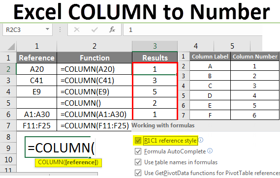
Example #1

We have a list of some cell addresses and a range of cells.

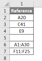
Now we will apply the COLUMN function here on the above cell address, and the Result is given below:

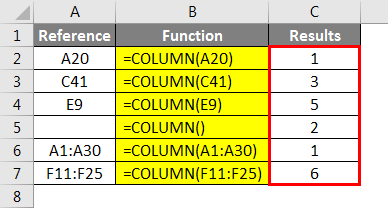
Explanation:

As we can see above, in cell B7, we have passed a blank argument inside the COLUMN function; hence it returns the number 2 as the COLUMN function itself exists in Column B.

Example #2

We have given below a list of references.

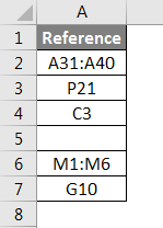
Now, after applying the COLUMN function, the final result is given below:

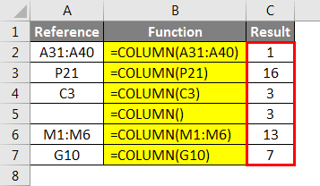
In the same way, we can find out the list of all column labels in excel. Below is the list from Column A: Column Z for your reference:

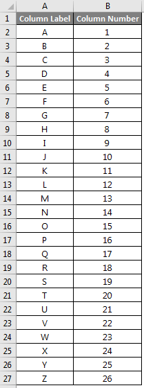
In an Excel spreadsheet named “Column A to Column ZZ”, we have provided you with the Column numbers from Column A to Column ZZ.

How to Change the Excel Reference Style?

Excel displays the column labels alphabetically, but we can change them with column numbers. This whole thing is called Excel R1C1 reference style.

For changing this reference style, please follow below steps:

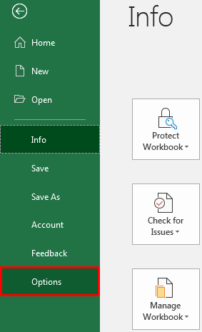
Open a Microsoft Excel spreadsheet, then go to the FILE tab and click on the Options tab in the left pane window, as shown in the below screenshot.

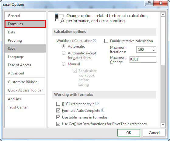
It will open an Excel options dialog box and click on the Formulas tab in the left pane window, as shown in the below screenshot.

This will display some options in the right side window, as you can see in the above image. Tick on checkbox R1C1 reference style under the Working with formulas section. Refer to the below screenshot.

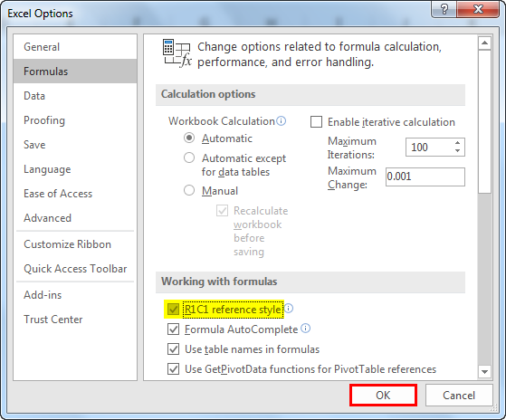
By clicking on this option, we enable the style of using numbers for both rows and columns. By default, Excel will display Column headings as Column alphabets. With this option, cells are referred to in this format: R1C1; click on OK.

As a result, Excel will convert the column labels into numbers. Refer to the below screenshot.

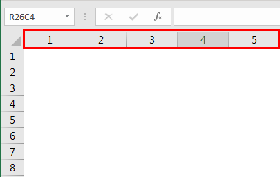
This R1C1 reference style option is disabled by default due to this Excel display column headings as alphabets.

What is the R1C1 Reference Style?

Excel, by default, uses the A1 reference style, which refers to Columns as letters. A is the column, and 1 in the row. Excel has a total of 256 columns and 65,536 rows.

i.e. 256 are the column headings, and 65,536 are the row numbers. For any cell address, we always start with a Column label followed by a Row number.

For Example, E65 refers to the cell where Column E and Row no. 65 intersect to each other.

We can convert the Column Labels into Column numbers by enabling the R1C1 reference style option under the FILE tab. This style is very useful when we are using rows and columns positions in macros.

In this R1C1 style, Excel refers to a cell position with “R” followed by a row a number and “C” followed by a column number.

Things to Remember About Excel Column to Number

Reference argument can be a single cell address or range of cells.
It is an optional argument, which means if we don’t pass any argument, it returns the column number of the cell where the column function exists.
This R1C1 reference style option is very useful when we are using row and column positions in macros.

How to change Excel column index from letter to number?

Open your spreadsheet.
Click on the orb button.
Click on Excel Options and move to the Formula tab.
Go to the Working with formulas section.
Check the R1C1 reference style. Note : Upon hovering your mouse cursor on it, you shall get all the information about this feature.
Click on OK.

Do you need more help with Excel? Check out our forum!

Источник

It’s common to find numbers stored as text in Excel. This leads to incorrect calculations when you use these cells in Excel functions such as SUM and AVERAGE (as these functions ignore cells that have text values in it). In such cases, you need to convert cells that contain numbers as text back to numbers.

Now before we move forward, let’s first look at a few reasons why you may end up with a workbook that has numbers stored as text.

Using ‘ (apostrophe) before a number.
- A lot of people enter apostrophe before a number to make it text. Sometimes, it’s also the case when you download data from a database. While this makes the numbers show up without the apostrophe, it impacts the cell by forcing it to treat the numbers as text.
Getting numbers as a result of a formula (such as LEFT, RIGHT, or MID)
- If you extract the numerical part of a text string (or even a part of a number) using the TEXT functions, the result is a number in the text format.

Now, let’s see how to tackle such cases.

Convert Text to Numbers in Excel

In this tutorial, you’ll learn how to convert text to numbers in Excel.

The method you need to use depends on how the number has been converted into text. Here are the ones that are covered in this tutorial.

Using the ‘Convert to Number’ option.
Change the format from Text to General/Number.
Using Paste Special.
Using Text to Columns.
Using a Combination of VALUE, TRIM, and CLEAN function.

Convert Text to Numbers Using ‘Convert to Number’ Option

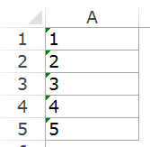
When an apostrophe is added to a number, it changes the number format to text format. In such cases, you’ll notice that there is a green triangle at the top left part of the cell.

In this case, you can easily convert numbers to text by following these steps:

Select all the cells that you want to convert from text to numbers.
Click on the yellow diamond shape icon that appears at the top right. From the menu that appears, select ‘Convert to Number’ option.

This would instantly convert all the numbers stored as text back to numbers. You would notice that the numbers get aligned to the right after the conversion (while these were aligned to the left when stored as text).

Convert Text to Numbers by Changing Cell Format

When the numbers are formatted as text, you can easily convert it back to numbers by changing the format of the cells.

Here are the steps:

Select all the cells that you want to convert from text to numbers.
Go to Home –> Number. In the Number Format drop-down, select General.

This would instantly change the format of the selected cells to General and the numbers would get aligned to the right. If you want, you can select any of the other formats (such as Number, Currency, Accounting) which will also lead to the value in cells being considered as numbers.

Also read: How to Convert Serial Numbers to Dates in Excel

Convert Text to Numbers Using Paste Special Option

To convert text to numbers using Paste Special option:

Convert Text to Numbers Using Text to Column

This method is suitable in cases where you have the data in a single column.

Here are the steps:

Select all the cells that you want to convert from text to numbers.
Go to Data –> Data Tools –> Text to Columns.
In the Text to Column Wizard:

While you may still find the resulting cells to be in the text format, and the numbers still aligned to the left, now it would work in functions such as SUM and AVERAGE.

Convert Text to Numbers Using the VALUE Function

You can use a combination of VALUE, TRIM and CLEAN function to convert text to numbers.

VALUE function converts any text that represents a number back to a number.
TRIM function removes any leading or trailing spaces.
CLEAN function removes extra spaces and non-printing characters that might sneak in if you import the data or download from a database.

Suppose you want convert cell A1 from text to numbers, here is the formula:

=VALUE(TRIM(CLEAN(A1)))

If you want to apply this to other cells as well, you can copy and use the formula.

Finally, you can convert the formula to value using paste special.

You May Also Like the Following Excel Tutorials:

Multiply in Excel Using Paste Special.
How to Convert Text to Date in Excel (8 Easy Ways)
How to Convert Numbers to Text in Excel
Convert Formula to Values Using Paste Special.
Excel Custom Number Formatting.
Convert Time to Decimal Number in Excel
Change Negative Number to Positive in Excel
How to Capitalize First Letter of a Text String in Excel
Convert Scientific Notation to Number or Text in Excel
How To Convert Date To Serial Number In Excel?

Источник

1. Select a column

2. Click this button

3. Click Apply

4. Set the format

Other ways to convert:

1. Insert a new column

2. Use the VALUE function

3. Rest your cursor here

4. Click and drag down

Related topics

Need more help?

Want more options?

How do I show column numbers in Excel?

How do I convert text to values in Excel?

How do I convert a column of numbers to column names in Excel?

How do I change the number format in Excel?

Why does Excel have numbers for columns?

How do I show columns and row numbers in Excel?

How do I get columns and row numbers in Excel?

How do I get row numbers in Excel?

How do I format numbers in Excel?

What are the different ways in formatting numbers?

How do I change the column title in Excel?

How do I change rows and column names in Excel?

How do I change Excel columns from numbers to alphabets?

How do I get rid of column 1 headers in Excel?

How do I change the row numbers in Excel?

What is an Xlookup in Excel?

Why can’t I see row numbers in Excel?

How do I add a numbered list in Excel?

How do I automatically number in sheets?

Excel COLUMN to Number

How to Use COLUMN Function in Excel?

Example #1

Example #2

How to Change the Excel Reference Style?

What is the R1C1 Reference Style?

Things to Remember About Excel Column to Number

Recommended Articles

How to change Excel column index from letter to number?

Convert Text to Numbers in Excel

Convert Text to Numbers Using ‘Convert to Number’ Option

Convert Text to Numbers by Changing Cell Format

Convert Text to Numbers Using Paste Special Option

Convert Text to Numbers Using Text to Column

Convert Text to Numbers Using the VALUE Function