Cells not formatting excel

When you fill out Excel worksheets with data, no one will succeed at once, everything is beautiful and correctly filled at the first attempt.

In the process of working with the program, you always need something: modify, edit, delete, copy or move. If the entered incorrect values in a cell, naturally, we want to correct or delete ones. But even such simple task can sometimes create difficulties.



How to set the cell format in Excel?

The contents of each Excel cell consist of three elements:

1. The meaning: text, numbers, dates and times, logical content, functions and formulas.
2. The formats: the type and color of the borders, the type and color of the fill, the way the values are displayed.
3. Comments.

All these three elements are completely independent of each other. You can specify the format of the cell and do not write anything to it, or add a note in an empty and not formatted cell.



How to change the format of cells in Excel?

To change the format of the cells, you should call the corresponding dialog box with the CTRL + 1 (or CTRL + SHIFT + F) key or from the context menu after you right-click the «Cell Format» option.

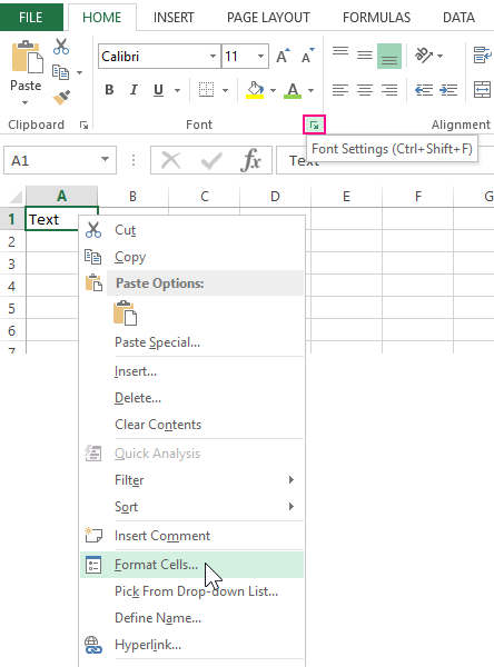
There are 6 tabs in this dialog box:

1. A number. Here you specify the way the numeric values are displayed.
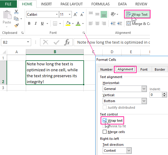
2. The alignment. On this tab you can control the position of the text. And the text can be displayed vertically or diagonally from any angle. Also pay attention to the «Display» section. Very often, the function «Wrap Text» is used.



3. Font. The specify the style design of fonts, the size and color of the text, plus the modes of modifications.
4. The border. Here you define the styles and colors of the borders. The design of all tables is better done right here.
5. The fill. The name of the bookmark speaks for itself. Available for formatting colors, patterns and methods of filling (for example, a gradient with a different direction of strokes).
6. The protection. Here, the cell protection settings are set, that are activated only after the protection of the whole sheet.

If you did not get the desired result on the first attempt, call this dialog again to fix the cell format in Excel.

What formatting is applicable to cells in Excel?

Each cell always has some format. If there were no changes, then this is the «General» format. It is also a standard Excel format, in which:

• the numbers are aligned on the right side;
• the text is aligned on the left side;
• the font Calibri with the height of 11 points;
• the cell has no borders and background fill.

The Format Removal – is the changing to the standard «General» format (without borders and fills).

It is worth noting that the format of cells, unlike values, can not be deleted with the DELETE key.

To delete the format of cells, select ones and use the «Clear Formats» tool, which is located on the «HOME» tab in the «Editing» section.

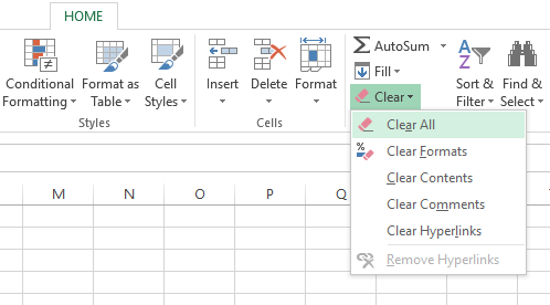
If you want to clear not only the format, but also the values, then select the «Clear All» option from the drop-down list of the tool (eraser).

As you can see, the eraser tool is functionally flexible and allows us to make a choice of what to delete in the cells:

• the content (same as the DELETE key);
• the formats;
• notes;
• the hyperlinks.

The option «Clear all» combines all these functions.

The deleting notes

Note, as well as formats, are not deleted from the cell by pressing the DELETE key. You can delete notes in two ways:

1. The eraser tool: the option «Clear notes».
2. Click on the cell with the note with the right mouse button, and from the appeared context menu select the option «Delete note».

The notation. The second way is more convenient. If you delete several notes at the same time, you must first select all of its cells.

A formatting issue in Excel may affect fonts, charts, shading, colors, borders, number formats, file formats, cell formats, hyperlink formats, and several other elements. For each of these different Excel format issues — Font Type and Size changed, Chart formatting, Conditional Formatting Rules, Text formatted to Number, Number formatted to Text or Date, Dates formatted to Numbers, etc. there are specific solutions.

A few common Excel formatting issues and how to fix them

1. Date Format issue in Excel:

The typed-in date changes to a number, text, another format of date (for example, MM/DD/YYYY may change to DD/MM/YYYY), or any other format that Excel does not recognize.

An example of Excel Date Format issue is as follows:

A user enters or types a Date — September 6 in a cell of Excel file. However, on pressing the ‘Enter’ key the value of the cell converts to a ‘Number.’

This implies that the cell’s number format is not in sync with what the user is trying to achieve. The cell is set to the Number format, which converts the input to a numerical value.

Solution: Right-click the cell containing the Date, select ‘Format Cells’, click ‘Date’ present under Number à Category and finally choose a Date format of choice (Example: DD/MM/YYYY format).

Note – This is valid for older versions of Excel.

In Excel 2007 and above versions; click a cell, next click the drop-down arrow in the Number section of the Home tab. In doing so, a list of the Number format appears, along with the data represented in each of the formats.

1. Number Format Issue and how to fix it

The Number format issue in Excel is an issue wherein a Number is formatted or changed to Text, Date, or any other format that is not recognized by Excel.

Solution: In such cases, users can use Error Checking or Paste Special as fixes.

1. Formatting issues in font type, size, color, and conditional formatting:

These generally occur in Excel if users open Excel files on a system other than where those were created, or if the new system runs an older Office/Excel version.

Solution: Users should make sure they save the Excel files in the native and widely accepted Excel 2007/2010 format, and not in the older Excel 97-2003 format. These are the options that users get while saving the Excel file using ‘Save As’ feature.

Users can also try to fix the Excel formatting issue by transferring all data from the current spreadsheet or workbook to a new and usable Excel workbook.

1. Excel XLS or XLSX file corruption:

In such situations, the Excel files need to be repaired which can be done by using either the inbuilt ‘Open or Repair’ utility or an Excel file repair software such as Stellar Repair for Excel.

The software repairs the damaged Excel (XLS or XLSX) file in 3 quick and easy steps: Select, Scan, and Save. You can save the repaired file either at the default or desired location.

Conclusion

Despite being an amazing application that allows users to create and process complex data in workbooks. Microsoft Excel is not free from concerns including the ones that arise due to formatting issues. This is true for all Excel versions, be it the latest Excel 2016 or other lower versions. Therefore, the need to employ the appropriate fixes whenever required.

In addition, the use of an advanced Excel repair tool is recommended to fix issues that appear due to Excel file corruption. An advanced software such as Stellar Repair for Excel recovers the lost formatting from corrupt Excel files. It offers an intuitive interface to repair Font formatting, Chart Formatting, Conditional formatting rules and more while preserving the data format at the time of restoring the Excel files.

Bill has a large worksheet that he can no longer format cells within. When he right-clicks on a cell and selects Format, the Format Cells dialog box never appears. Likewise, if he chooses Cells from the Format menu, the dialog box never shows up.

This, obviously, is not the way that Excel is supposed to behave. Since the problem occurs with only a single workbook, the problem is most likely not with Excel itself, but with the workbook. There are a few things you can try to track down the problem.

First, make sure that you open the workbook with macros disabled. Hold down the Shift key as you double-click the workbook in Windows Explorer, then indicate that you don’t want to enable the macros. If the problem persists, you can rule out it being rooted in a macro. If the problem goes away, then you know you need to examine the macros to see which one is causing the problem.

Second, the file (which Bill mentions is both old and large) could have so many formats defined within it that you can no longer do formatting. This problem has been covered in other issues of ExcelTips, and you can find related information, including a way to free up formats, here:

https://bettersolutions.com/excel/formatting/vba-delete-unused-custom-formats.htm

https://answers.microsoft.com/en-us/office/forum/office_2007-excel/delete-custom-formats/23d6727c-d052-e011-8dfc-68b599b31bf5?db=5

Look for the macro entitled DeleteUnusedCustomNumberFormats; it can help clean up the no-longer-used custom formats.

Another thing to try is to save the worksheet as an HTML file, get out of Excel, get back into the program, and then load the HTML file. Sometimes the «round trip» for a worksheet will clear up some quirks that may be confusing Excel.

Author Bio

With more than 50 non-fiction books and numerous magazine articles to his credit, Allen Wyatt is an internationally recognized author. He is president of Sharon Parq Associates, a computer and publishing services company. Learn more about Allen…

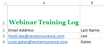
I am unable to format a column into date format unless I click into the cell then click out.

This data is exported from a third party application to .xlsx format. When I open the file in Excel and try to format what should be the date column, the date formatting will not take affect until I click into the cell as if I were going to make changes then exit/click out of the cell.

Image 1 raw data

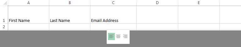
image 2 setting the formatting

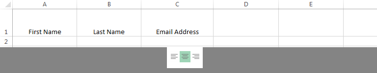
image 3, clicking into a cell.

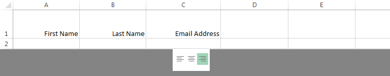
image 4, clicking out of the cell.

Notice the rest of the rows in image 4 that rows 4 and beyond have retained their original formatting, and the only ones that have the new formatting are the ones I clicked into then clicked out. Selecting a cell without going into it also keeps the original formatting. While clicking into a cell then out is not a huge problem, when you get thousands of rows this gets annoying. Any fix or workaround you can suggest?

/en/excel2013/modifying-columns-rows-and-cells/content/

Introduction

All cell content uses the same formatting by default, which can make it difficult to read a workbook with a lot of information. Basic formatting can customize the look and feel of your workbook, allowing you to draw attention to specific sections and making your content easier to view and understand. You can also apply number formatting to tell Excel exactly what type of data you’re using in the workbook, such as percentages (%), currency ($), and so on

Optional: Download our practice workbook.

To change the font:

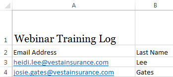
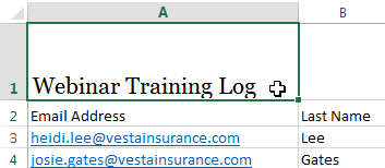
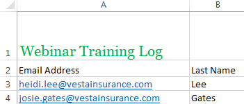
By default, the font of each new workbook is set to Calibri. However, Excel provides many other fonts you can use to customize your cell text. In the example below, we’ll format our title cell to help distinguish it from the rest of the worksheet.

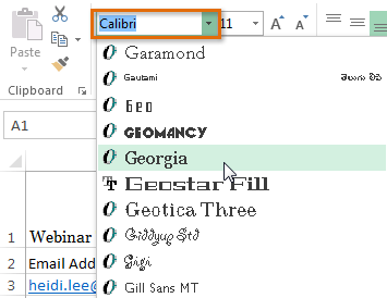
1. Select the cell(s) you want to modify.

   Selecting a cell

2. Click the drop-down arrow next to the Font command on the Home tab. The Font drop-down menu will appear.
3. Select the desired font. A live preview of the new font will appear as you hover the mouse over different options. In our example, we’ll choose Georgia.

   Choosing a font
   

4. The text will change to the selected font.

   The new font

When creating a workbook in the workplace, you’ll want to select a font that is easy to read. Along with Calibri, standard reading fonts include Cambria, Times New Roman, and Arial.

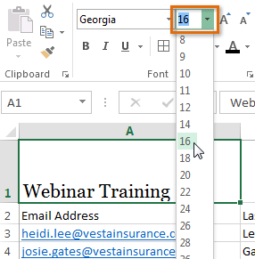
To change the font size:

1. Select the cell(s) you want to modify.

   Selecting a cell

2. Click the drop-down arrow next to the Font Size command on the Home tab. The Font Size drop-down menu will appear.
3. Select the desired font size. A live preview of the new font size will appear as you hover the mouse over different options. In our example, we will choose 16 to make the text larger.

   Choosing a new font size

4. The text will change to the selected font size.

   The new font size

You can also use the Increase Font Size and Decrease Font Size commands or enter a custom font size using your keyboard.

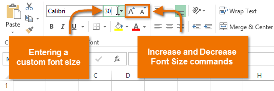Modifying the font size

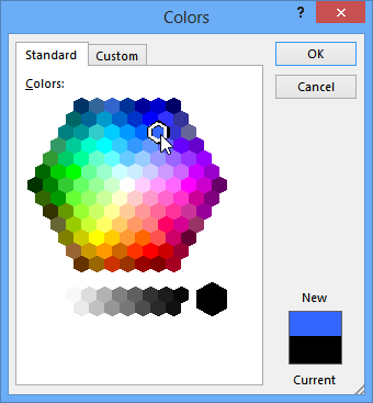
To change the font color:

1. Select the cell(s) you want to modify.

   Selecting a cell

2. Click the drop-down arrow next to the Font Color command on the Home tab. The Color menu will appear.
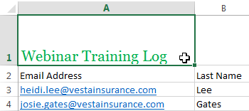
3. Select the desired font color. A live preview of the new font color will appear as you hover the mouse over different options. In our example, we’ll choose Green.

   Choosing a font color

4. The text will change to the selected font color.

   The new font color

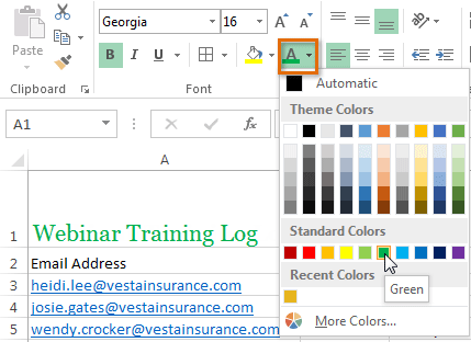
Select More Colors at the bottom of the menu to access additional color options.

Selecting more colors

To use the Bold, Italic, and Underline commands:

1. Select the cell(s) you want to modify.

   Selecting a cell

2. Click the Bold (B), Italic (I), or Underline (U) command on the Home tab. In our example, we’ll make the selected cells bold.

   Clicking the Bold command

3. The selected style will be applied to the text.

   The bold text

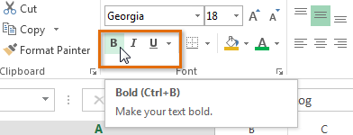
You can also press Ctrl+B on your keyboard to make selected text bold, Ctrl+I to apply italics, and Ctrl+U to apply an underline.

Text alignment

By default, any text entered into your worksheet will be aligned to the bottom-left of a cell, while any numbers will be aligned to the bottom-right. Changing the alignment of your cell content allows you to choose how the content is displayed in any cell, which can make your cell content easier to read.

Click the arrows in the slideshow below to learn more about the different text alignment options.

• 

  Left align: Aligns content to the left border of the cell

• 

  Center align: Aligns content an equal distance from the left and right borders of the cell

• 

  Right Align: Aligns content to the right border of the cell

• 

  Top Align: Aligns content to the top border of the cell

• 

  Middle Align: Aligns content an equal distance from the top and bottom borders of the cell

• 

  Bottom Align: Aligns content to the bottom border of the cell

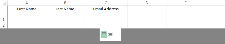
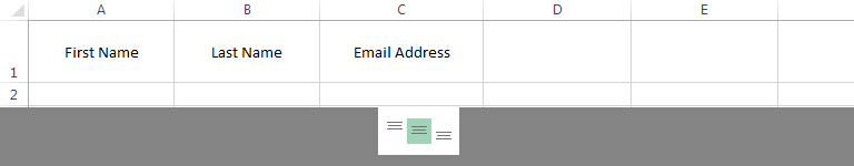
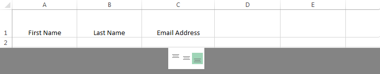
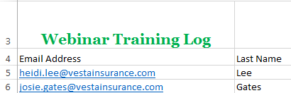
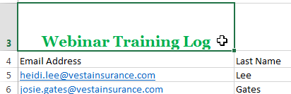
To change horizontal text alignment:

In our example below, we’ll modify the alignment of our title cell to create a more polished look and further distinguish it from the rest of the worksheet.

1. Select the cell(s) you want to modify.

   Selecting a cell

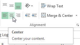
2. Select one of the three horizontal alignment commands on the Home tab. In our example, we’ll choose Center Align.

   Choosing Center Align

3. The text will realign.

   The realigned cell text

To change vertical text alignment:

1. Select the cell(s) you want to modify.

   Selecting a cell

2. Select one of the three vertical alignment commands on the Home tab. In our example, we’ll choose Middle Align.

   Choosing Middle Align

3. The text will realign.

   The realigned cell text

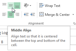
You can apply both vertical and horizontal alignment settings to any cell.

Cell borders and fill colors

Cell borders and fill colors allow you to create clear and defined boundaries for different sections of your worksheet. Below, we’ll add cell borders and fill color to our header cells to help distinguish them from the rest of the worksheet.

To add a border:

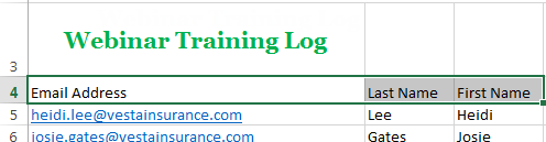
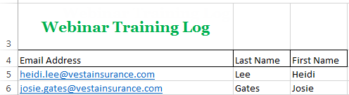
1. Select the cell(s) you want to modify.

   Selecting a cell range

2. Click the drop-down arrow next to the Borders command on the Home tab. The Borders drop-down menu will appear.
3. Select the border style you want to use. In our example, we will choose to display All Borders.

   Choosing a border style

4. The selected border style will appear.

   The added cell borders
   

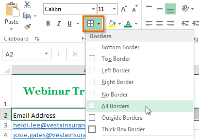
You can draw borders and change the line style and color of borders with the Draw Borders tools at the bottom of the Borders drop-down menu.

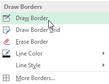Drawing custom borders

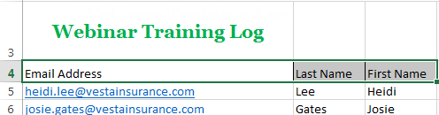
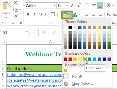
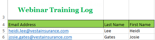
To add a fill color:

1. Select the cell(s) you want to modify.

   Selecting a cell range

2. Click the drop-down arrow next to the Fill Color command on the Home tab. The Fill Color menu will appear.
3. Select the fill color you want to use. A live preview of the new fill color will appear as you hover the mouse over different options. In our example, we’ll choose Light Green.

   Choosing a cell fill color

4. The selected fill color will appear in the selected cells.

   The new fill color

Format Painter

If you want to copy formatting from one cell to another, you can use the Format Painter command on the Home tab. When you click the Format Painter, it will copy all of the formatting from the selected cell. You can then click and drag over any cells you want to paste the formatting to.

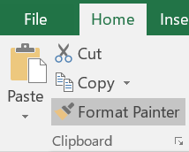
Watch the video below to learn two different ways to use the Format Painter.

Cell styles

Instead of formatting cells manually, you can use Excel’s predesigned cell styles. Cell styles are a quick way to include professional formatting for different parts of your workbook, such as titles and headers.

To apply a cell style:

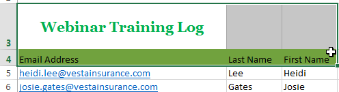
In our example, we’ll apply a new cell style to our existing title and header cells.

1. Select the cell(s) you want to modify.

   Selecting a cell range

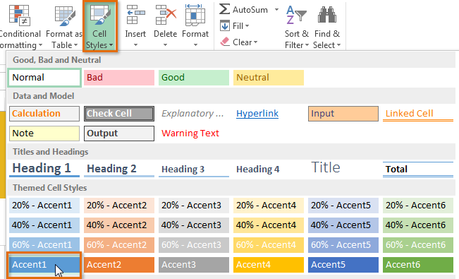
2. Click the Cell Styles command on the Home tab, then choose the desired style from the drop-down menu. In our example, we’ll choose Accent 1.

   Choosing a cell style

3. The selected cell style will appear.

   The new cell style

Applying a cell style will replace any existing cell formatting except for text alignment. You may not want to use cell styles if you’ve already added a lot of formatting to your workbook.

Formatting text and numbers

One of the most powerful tools in Excel is the ability to apply specific formatting for text and numbers. Instead of displaying all cell content in exactly the same way, you can use formatting to change the appearance of dates, times, decimals, percentages (%), currency ($), and much more.

To apply number formatting:

In our example, we’ll change the number format for several cells to modify the way dates are displayed.

1. Select the cells(s) you want to modify.

   Selecting a cell range

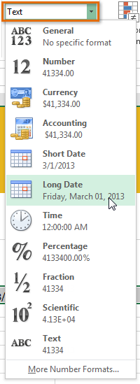
2. Click the drop-down arrow next to the Number Format command on the Home tab. The Number Formatting drop-down menu will appear.
3. Select the desired formatting option. In our example, we will change the formatting to Long Date.

   Choosing Long Date
   

4. The selected cells will change to the new formatting style. For some number formats, you can then use the Increase Decimal and Decrease Decimal commands (below the Number Format command) to change the number of decimal places that are displayed.

   The applied number formatting

Click the buttons in the interactive below to learn about different text and number formatting options.

Challenge!

1. Open an existing Excel 2013 workbook. If you want, you can use our practice workbook.
2. Select a cell and change the font style, size, and color of the text. If you are using the example, change the title in cell A3 to Verdana font style, size 16, with a font color of green.
3. Apply bold, italics, or underline to a cell. If you are using the example, bold the text in cell range A4:C4.
4. Try changing the vertical and horizontal text alignment for some cells.
5. Add a border to a cell range. If you are using the example, add a border to the header cells in in row 4.
6. Change the fill color of a cell range. If you are using the example, add a fill color to row 4.
7. Try changing the formatting of a number. If you are using the example, change the date formatting in cell range D4:H4 to Long Date.

/en/excel2013/worksheet-basics/content/