
Does your Excel cell content not visible but show in formula bar? Don’t have any idea why is the text not showing in Excel cells?
Want to know how you can solve this Excel text disappears in cell mystery?
In that case, this particular post is very important to read. As it contains complete detail on how to fix Excel cell contents not visible issues.
User’s Query:
Let’s understand this issue more clearly with these user complaints.
Issue: Content of Excel cells invisible while typing
If I’m typing text or numbers into an Excel cell, while I can see what I’m writing in the formula bar above the chart, the cell shows nothing but the vertical stroke of a cursor, and no text or numbers at all until I tab out of the cell. I find this very annoying, though not a stopper to doing work. It’s unlike any Excel I’ve used in the past.
Source: https://answers.microsoft.com/en-us/msoffice/forum/all/content-of-excel-cells-invisible-while-typing/7937a331-4b27-4790-adda-9341d2010f10?auth=1
To recover lost Excel cell contents, we recommend this tool:
This software will prevent Excel workbook data such as BI data, financial reports & other analytical information from corruption and data loss. With this software you can rebuild corrupt Excel files and restore every single visual representation & dataset to its original, intact state in 3 easy steps:
- Download Excel File Repair Tool rated Excellent by Softpedia, Softonic & CNET.
- Select the corrupt Excel file (XLS, XLSX) & click Repair to initiate the repair process.
- Preview the repaired files and click Save File to save the files at desired location.
These are the fixes that you all must try to get rid of the issue Excel cell contents not visible but show in formula bar.
1# Set The Cell Format To Text
2# Display Hidden Excel Cell Values
3# Using The Autofit Column Width Function
4# Display Cell Contents With Wrap Text Function
5# Adjust Row Height For Cell Content Visibility
6# Reposition Cell Content By Modifying The Alignment Or Rotating Text
7# Retrieve Missing Excel Cell Content
Let’s discuss all these fixes in detail….!
Fix 1# Set The Cell Format To Text
If you are facing this Excel cell contents not visible issue with a particular formula. Even after checking the formula, you haven’t found any error but still, it not showing the result.
- In that case, immediately check whether the cell format is set to text or not.
- You can also set the format of the cell to another suitable number format.
- Now you need to get into the “cell edit mode” so that Excel can easily identify the format modification. For this just make a tap on the formula bar and hit enter.
Fix 2# Display Hidden Excel Cell Values
- Choose either the range of the cell or the cells having hidden values.
Tip: you can easily cancel the cell selection, by tapping any cell present on the Excel worksheet.
- Go to the Home tab and hit the Dialog Box Launcher which is present next to the Number.

- Now from the Category box, tap to the General for application of the default number format.

Just tap on the number, date, or time, a format that you require.
Fix 3 # Using The Autofit Column Width Function
To display all the text not showing in Excel cell you can use the function Autofit Column Width.
It’s a very helpful feature to make easy adjustments in the column width of the cells. So this feature will, ultimately going to help in displaying all the hidden Excel cells content.
Here are the steps which you need to perform.
- Choose the cell having hidden excel cell content and follow this path Home> Format > AutoFit Column Width.

- After this, you will see all the cells of your worksheet will adjust their respective column width. This ultimately shows all the hidden Excel cell text.

Fix 4# Display Cell Contents With Wrap Text Function
With the Excel wrap text feature you can apply such cell formatting in which text will get wrap automatically or put a line break. After using the wrap text function your hidden excel cell content will start appearing in multiple lines.
- Choose that cell whose content is not visible and tap to the Home> Wrap Text

- After that, you will see your selected cell will be expanded with all the hidden content. Like this:

Note:
If still your Excel cell content not visible completely then maybe it’s because of the row size which is set to some specific height.
So follow the next solution of changing the row height to perfect content visibility.
Fix 5# Adjust Row Height For Cell Content Visibility
- You can choose single or multiple rows in which you want to make a row height changes.
- Go to the Home tab. Now from the Cells group choose the Format option.
- Within the Cell Size, tap to the AutoFit Row Height.
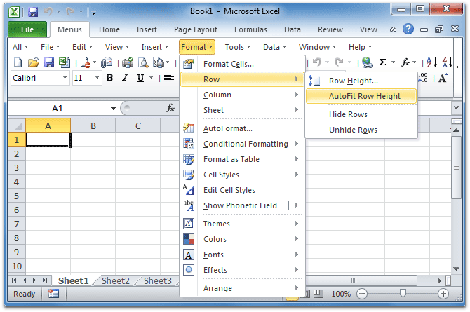
Note: for quick autofit row height of the entire worksheet cells. Just tap to the Select All button. After that make double-tap on the boundary present just below the row heading.
Fix 6# Reposition Cell Content By Modifying The Alignment Or Rotating Text
For the perfect display of data in the worksheet, you must try repositioning the text present within the cell. For this, you can make modifications in the alignment of the cell content or you can use the indentation for correct spacing. Or else display the cell content at various angles by rotating it.
1. Select the range of the cells having the data which you wish to reposition.
2. Now make a right-click over the selected rows, you will get a list of options. From which you have to choose format cells.

3. In the opened dialog box of Format Cells choose the Alignment tab and perform any of the following operations:
- Change the horizontal alignment of the cell contents
- Change the vertical alignment of the cell contents
- Indent the cell contents
- Display the cell contents vertically from top to bottom
- Rotate the text in a cell
- Restore the default alignment of selected cells

Fix 7# Retrieve Missing Excel Cell Content
Another very high possibility of having this Excel cell content not visible issue is worksheet corruption. As it is found that data from Excel sheet goes missing when Excel file or worksheet got corrupted.
So either you can try the manual fixes to recover corrupt Excel file data. Or else go with experts recommended solution for recovery i.e Excel repair software.
Have a look over some catchy features of this software:
- This supports the entire Excel version and the demo version is free.
- This is a unique tool to repair multiple Excel files at one repair cycle and recovers the entire data in a preferred location.
- This is unique software to repair multiple files at once and recover everything in the preferred location.
- It is easy to use and compatible with both Windows as well as Mac operating systems.
- With the help of this, you can fix all sorts of issues, corruption, errors in Excel workbooks.
Wrap Up:
By trying the above-mentioned fixes you can easily fix Excel cell contents not visible but show in formula bar issue. But even if the fixes fail to display hidden Excel cell content then immediately approach the software solution.
Don’t do unnecessary delay as this will lessen the possibility of complete Excel worksheet data recovery.


Priyanka is an entrepreneur & content marketing expert. She writes tech blogs and has expertise in MS Office, Excel, and other tech subjects. Her distinctive art of presenting tech information in the easy-to-understand language is very impressive. When not writing, she loves unplanned travels.
Sometimes, when you open an Excel spreadsheet, you can’t see the text you have typed in a cell.
The text may be visible on the formula bar but not in the cell itself. For instance, in the image below, the data in cell C2 is not visible but you can see it in the formula bar.
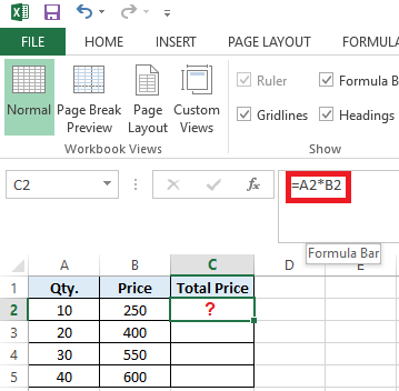
Figure 1 — Excel Not Showing Data in Cells
Also Read: Data Disappears in Excel – How to Get it Back?
Workarounds to Fix ‘Excel Not Showing Data in Cells’
Note: Before trying these workarounds, make sure that your Office program is updated.
Workaround 1 – Check for Hidden Cell Values
If cell values are hidden, you won’t be able to see data when a cell is selected. But the data will be visible in the formula bar. To display hidden cell values in a worksheet, follow these steps:
- Select a single cell or range of cells that doesn’t show the text.
- Right-click on the selected cell or range of cells and choose Format Cells.
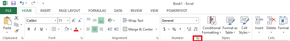
Figure 2 — Select Format Cells
- A ‘Format Cells’ window opens. On the Number tab, choose Custom and check if 3 semi-colons (;;;) appear in the Type textbox.
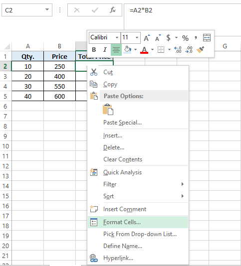
Figure 3 — Check for Semi-Colons in Type Box
- If you can see the 3 semi-colons, delete them and then click OK. If you cannot see semi-colons in the ‘Type’ textbox, skip to the next workaround.
Workaround 2 – Change the Default Font
The font of cells in your Excel worksheet may be creating the problem. So, try changing the default font of cells or ranges:
- Select a cell or cell range where the text is not showing up.
- Right-click on the selected cell or cell range and click Format Cells.
- From the pop-up window, click on the Font tab and then change the default font (usually Calibri) to any other font, like ‘Arial’ or ‘Times New Roman’. Press the OK button.
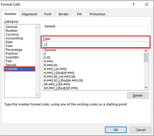
Figure 4 – Format Cells Window
If changing the default font doesn’t fix the ‘Excel data not showing in cell’ problem, proceed with the next workaround.
Workaround 3 – Disable Allow Editing Directly in Cell Option
Some users have reported that they were able to resolve the ‘Excel data not showing in cells’ issue by unchecking the ‘Allow editing directly in cells’ option. To do so, follow these steps:
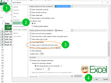
- In Excel, click on the File menu and then click on Options.
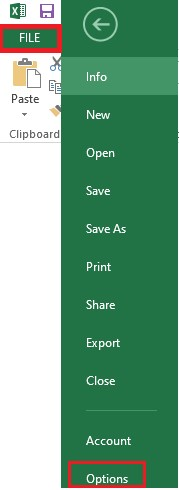
Figure 5 — Excel Options
- From the Excel Options window, choose Advanced in the left pane and then uncheck ‘Allow editing directly in cells’.
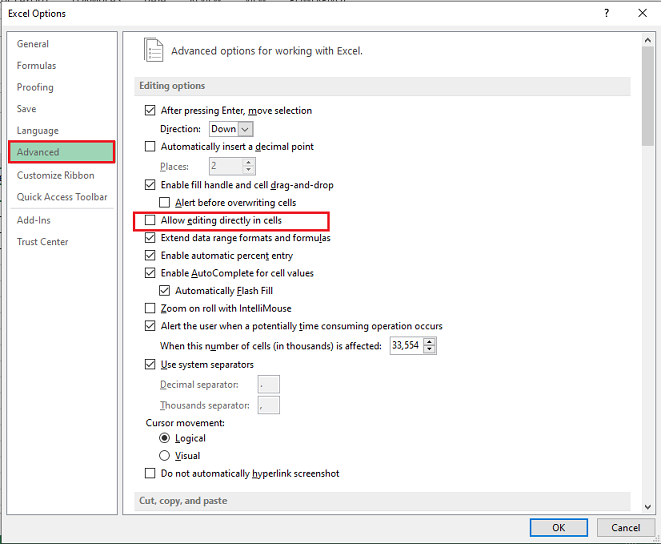
Figure 6 — Uncheck Allow Editing Directly in Cells
- Click OK.
If you are unable to view the text in Excel cells, try the next workaround.
Workaround 4 – Adjust Row Height to Make the Cell Data Visible
If you have cells with wrapped text, then try adjusting the row height of the cell or range to make the data visible. Here are the steps:
- Select a specific cell or range for adjusting the row height.
- On the Home tab, click Format from the Cells group.
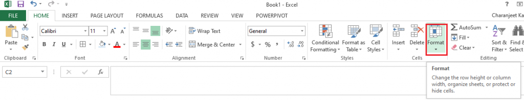
Figure 7 — Format Option in Cells Group
- Under Cell Size, perform any of these actions:
- Click AutoFit Row Height to automatically adjust the row height of your cell or cell range.
- Click Row Height to manually enter a cell’s row height. This will open a ‘Row Height’ box. In the box, enter the row height that you want.
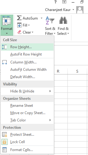
Figure 8 – Cell Size Options
Tip: You can also adjust a cell’s row height by dragging the bottom border of the row till the height when the wrapped text is visible.
Workaround 5 – Recover Missing Cell Content
Your Excel worksheet won’t display data in cells if it is corrupted. In other words, the cell values won’t display any result if the data in your Excel worksheet is damaged or corrupted. In that case, you can manually fix and recover corrupt Excel files or use an Excel repair tool, such as Stellar Repair for Excel.

Read this: How to Recover Corrupted Excel File?
Using the Excel file repair tool can help you retrieve all your worksheet data, including cell content, tables, numbers, text, rules, etc.
Wrapping Up
Oftentimes, when opening an Excel worksheet or while working on one, clicking on a cell or cell range doesn’t show any data. You may be able to see the data in the formula bar of your worksheet but not within the cells. This may prevent you from doing anything constructive in Excel. Try troubleshooting the issue by using the workarounds discussed in this article. If nothing works, chances are that corruption in the Excel file is causing it to behave oddly. Try repairing corrupt Excel file by using the built-in ‘Open and Repair’ feature or use Excel file repair software by Stellar to quickly restore your worksheet with all its data intact.
You might also be interested in reading:
[Fix] Excel formula not showing result
Easy Steps to Make Excel Hyperlinks Working
One of my customers, faced the following strange problem when he opens several Excel files: The Excel file seem to open normally, but the Excel won’t show the worksheet (Worksheet area is grayed out and the data doesn’t appear at all). As a first try, I repaired the MS Office (2007) installation but the problem still exists. Finally after some research I found the following solution to resolve the «Excel Worksheet data not showing» problem.
How to fix: Excel Data not showing – not visible – data area is grayed out.
1. Go to View Menu and ensure first that the Unhide option is inactive. (otherwise click Unhide and check if you can view the excel data).
2. Select Arrange All.

3. At the menu that comes up, check the «Windows of active workbook» checkbox and click OK.

Now you should see the contents of the Excel Workbook!
4. One last action. Save the Workbook and you ‘re done!
Additional help: If the above tip doesn’t help you, then:
A. Perform a repair at Office installation. To do that:
- Navigate to Windows Control Panel > Programs and features.
- Locate and select the MS Office application and then click Change.
- Then select the Repair option.
B. Disable the Hardware Acceleration at Excel application: To do that:
Notice: The option to disable the graphics acceleration is only available at Excel 2010 and Excel 2013.
1. From Excel’s main menu select Options.

2. At Excel Options window, choose Advanced on the left pane.

3. At the right pane, under Display options, uncheck the «Disable hardware graphics acceleration» checkbox and click OK.

That’s all folks! Did it work for you?
Please leave a comment in the comment section below or even better: like and share this blog post in the social networks to help spread the word about this solution.
If this article was useful for you, please consider supporting us by making a donation. Even $1 can a make a huge difference for us.

I have a customer which is using 2010 and having this issue on a daily basis. They are rebooting every night, but when they use the spreadsheet the following day the issue returns, but changes from day to day. The first time they showed the issue to me it was not placing borders around columns D-G when they selected a row, then the next time it’s a different set of columns. I’ve not seen it duplicate the issue for the same set of columns. Nor do the unbordered columns remain the same throughout the day. What’s odd is if the user Alt/Tab’s to a different window, then returns back to the workbook, the selected cells will display the proper borders until the active cell is changed. The workbook contains 2 worksheets, 1 macro, and one pivot table. The largest worksheet only contains approximately 150 row and makes use of 12 columns. When I bring the workbook onto my 2013 system I find no issues. Have searched the internet for a resolution but have had no luck. This thread is the closest I’ve found to others that have had a similar issue. Any ideas, thoughts, or suggestions would be appreciated. Thank you in advance for your communications.
I have a table where track data on a daily base, compare it to a daily target I have set, calculate the gap between the two and display the data on a line chart.
The data has 4 columns:
A. Date (from today until 31-12-2014
C. Actual value (only filled for past dates)
D. Target Value (all filled until 31-12-2014)
E. Gap (C-D)
I wanted the Gap (E) to be empty as long as there is no current date, and thus filled it with the formula:
=IF(ISBLANK(C10), "", C10-D10)
The future dates of Column E correctly display blank.
When I create a chart from the data (with E being on a different axis), the line is not drawn for future dates of column C since the values are blank, but they are drawn for future dates of column E with Zero.
I am assuming that the result of the formula with a «» content of the field is not considered as «blank» so that the chart assumes it to be zero.
How can I make the line of the chart in Column E disappear for dates where there is no value in Column C (and therefore also in Column E)?
This tutorial solves a problem where Excel won’t allow you to insert new rows or columns in a worksheet. When you try this, Excel displays the message “Microsoft Excel can’t insert new cells because it would push non-empty cells off the end of the worksheet. Those non-empty cells might appear empty but have blank values, some formatting or a formula. Delete enough rows or columns to make room for what you want to insert and then try again.”
5 FREE EXCEL TEMPLATES
Plus Get 30% off any Purchase in the Simple Sheets Catalogue!
METHOD 1: Clear Last Row or Column
The most probable reason you are getting this message is that in the last row or column of your worksheet, there is either formatting, data or a formula. This might not be easy to spot, but by following the instructions below you can easily clear the offending cells.
A quick way to navigate to the last column in your worksheet is to:
- Click somewhere in the first empty column in your worksheet (to the right of any data)
- Use the key combination CTRL ⇒ (CTRL and the right-arrow key)
A quick way to navigate to the last row in your worksheet is to:
- Click somewhere in the first empty row in your worksheet (below any data)
- Use the key combination CTRL ⇓ (CTRL and the down-arrow key)
If you can see either data, a formula or formatting in the last row or column, this is probably where the problem lies.
Here is a fairly reliable way to clear all cells to the right of or below your data (including the last column and row):
- Select the whole of the first empty column in your worksheet (to the right of any data). You can quickly select the whole column by clicking on the column letter that appears at the top of the worksheet
- Use the key combination CTRL SHIFT ⇒ to select all columns to the right
- On the ribbon’s Home tab, in the Editing group, click the Clear button and then Clear All
- Now select the first empty row in your worksheet (below your data). You can quickly select the whole row by clicking on the row number that appears on the left of your worksheet
- Use the key combination CTRL SHIFT ⇓ to select all rows below
- On the ribbon’s Home tab, in the Editing group, click the Clear button and then Clear All
Once you have completed these steps, try inserting a row or column. You may get a warning message titled ‘Large Operation’. The warning indicates that inserting new cells may take a significant amount of time to complete. You can ignore the warning and click on OK.
METHOD 2: Copy to a New Worksheet
If the method above does not work, try this method:
- Create a new worksheet in your workbook
- Copy and paste your data into the new worksheet
- Insert the new column or row in the copy of your data
- Copy the copy of the data that now includes a new row or column
- Navigate back to the original worksheet
- Select the top left cell of the data that you originally copied
- Paste
You will need to repeat these steps for each column or row you need to insert.
METHOD 3: Clear the ‘Used Range’
If method 1 and 2 fail, Try method 3.
Method 3 requires you to reset the ‘used range’ in your worksheet. To do this:
- Use the key combination ALT F11 to open the Visual Basic Editor (VBE)
- Use the key combination CTRL G to open the Immediate window. The Immediate window appears near the bottom of the VBE with the title ‘Immediate’
- In the Immediate window type the following code: activesheet.usedrange.select
- Press ENTER on your keyboard
- Use the key combination ALT Q to close the VBE
- Now try inserting a new column or row in your worksheet
Watch Video – How to Highlight Blank Cells in Excel
When I get a data file from a client/colleague or I download it from a database, I do some basic checks on the data. I do this to make sure there are no missing data points, errors or duplicates that may lead to issues later.
One such check is to find and highlight blank cells in Excel.
There are many reasons that can result in blank cells in a dataset:
- The data is not available.
- Data points accidentally got deleted.
- A formula returns an empty string resulting in a blank cell.
While it’s easy to spot these blank cells in a small dataset, if you have a huge one with hundreds of rows and columns, doing this manually would be highly inefficient and error prone.
In this tutorial, I will show you various ways to find and highlight blank cells in Excel.
Highlight Blank Cells Using Conditional Formatting
Conditional Formatting is a great way to highlight cells based on its value when the given condition is met.
I am going to showcase these examples with a small dataset. However, you can use these same techniques with large datasets as well.
Suppose you have a dataset as shown below:
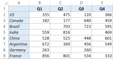
You can see there are blank cells in this dataset.
Here are the steps to highlight blank cells in Excel (using conditional formatting):
This would highlight all the blank cells in the dataset.

Note that conditional formatting is dynamic. This means that if conditional formatting is applied and you delete a data point, that cell would get highlighted automatically.
At the same time, this dynamic behavior comes with an overhead cost. Conditional Formatting is volatile, and if used on large data sets, may slow down your workbook.
Also read: Delete Blank Columns in Excel
Select and Highlight Blank Cells in Excel
If you want to quickly select and highlight cells that are blank, you can use the ‘Go to Special’ technique.
Here are the steps to select and highlight blank cells in Excel:
As mentioned, this method is useful when you want to quickly select all the blank cells and highlight it. You can also use the same steps to select all the blank cells and then fill 0 or NA or any other relevant text in it.
Note that unlike conditional formatting, this method is not dynamic. If you do it once, and then by mistake delete a data point, it will not get highlighted.
Using VBA to Highlight Blank Cells in Excel
You can also use a short VBA code to highlight blank cells in a selected dataset.
This method is more suitable when you need to often find and highlight blank cells in data sets. You can easily use the code below and create an add-in or save it in your personal macro workbook.
Here is the VBA code that will highlight blank cells in the selected dataset:
'Code by Sumit Bansal (https://trumpexcel.com)
Sub HighlightBlankCells()
Dim Dataset As Range
Set Dataset = Selection
Dataset.SpecialCells(xlCellTypeBlanks).Interior.Color = vbRed
End Sub
Here are the steps to put this VBA code in the backend and then use it to highlight blank cells in Excel:
How to Run the VBA code (Macro)?
Once you have copy pasted this macro, there are a couple of ways you can use this macro.
Using the Macro Dialog Box
Here are the steps to run this macro using the Macro dialog box:
- Select the data.
- Go to the Developer tab and click on Macros.

- In the Macro dialog box, select the ‘HighlightBlankCells’ macro and click on Run.


Using the VB Editor
Here are the steps to run this macro using the VB Editor:
- Select the data.
- Go to the Developer tab and click on Visual Basic.

- In the VB Editor, click anywhere within the code.
- Click on the Green triangle button in the toolbar (or hit the F5 key).


As I mentioned, using VBA macro to highlight blank cells is the way to go if you need to do this often.
Apart from the ways shown above to run the macro, you can also create an add-in or save the code in the Personal macro workbook.
This will allow you to access this code from any workbook in your system.
You May Also Like the Following Excel Tutorials:
- How to Find External Links and References in Excel.
- How to Quickly Find and Remove Hyperlinks in Excel.
- Highlight EVERY Other ROW in Excel.
- The Ultimate Guide to Find and Remove Duplicates in Excel.
- Using InStr Function in Excel VBA.
- How to Filter Cells with Bold Font Formatting in Excel.
- How to Compare Two Columns in Excel.
If the return cell in an Excel formula is empty, Excel by default returns 0 instead. For example cell A1 is blank and linked to by another cell. But what if you want to show the exact return value – for empty cells as well as 0 as return values? This article introduces three different options for dealing with empty return values.
Option 1: Don’t display zero values
Probably the easiest option is to just not display 0 values. You could differentiate if you want to hide all zeroes from the entire worksheet or just from selected cells.
There are three methods of hiding zero values.
- Hide zero values with conditional formatting rules.
- Blind out zeros with a custom number format.
- Hide zero values within the worksheet settings.
For details about all three methods of just hiding zeroes, please refer to this article.

One small advice on my own account: My Excel add-in “Professor Excel Tools” has a built-in Layout Manager. With this, you can apply this formatting easily to a complete Excel workbook.
Give it a try? Click here and the download starts right away.
Option 2: Change zeroes to blank cells
Unlike the first option, the second option changes the output value. No matter if the return value is 0 (zero) or originally a blank cell, the output of the formula is an empty cell. You can achieve this using the IF formula.

Say, your lookup formula looks like this: =VLOOKUP(A3,C:D,2,FALSE) (hereafter referred to by “original formula”). You want to prevent getting a zero even if the return value―found by the VLOOKUP formula in column D―is an empty value. This can be achieved using the IF formula.
The structure of such IF formula is shown in the image above (if you need assistance with the IF formula, please refer to this article). The original formula is wrapped within the IF formula. The first argument compares if the original formula returns 0. If yes―and that’s the task of the second argument―the formula returns nothing through the double quotation marks. If the orgininal formula within the first argument doesn’t return zero, the last argument returns the real value. This is achieved by the original formula again.
The complete formula looks like this.
=IF(VLOOKUP(A3,C:D,2,FALSE)=0,"",VLOOKUP(A3,C:D,2,FALSE))
Do you want to boost your productivity in Excel?
Get the Professor Excel ribbon!

Add more than 120 great features to Excel!
Option 3: Show zeroes but don’t show blank or empty return values

The previous option two didn’t differentiate between 0 and empty cells in the return cell. If you only want to show empty cells if the return cell found by your lookup formula is empty (and not if the return value really is 0) then you have to slightly alter the formula from option 2 before.
Like before, the IF formula is wrapped around the original formula. But instead of testing if the return value is 0, it tests within the first argument if the return value is blank. This is done by the double quotation marks. The rest of the formula is the as before: With the second argument you define that—if the value from the original formula is blank—the return value is empty too. If not, the last argument defines that you return the desired non-blank value.
The formula in your example from option 2 looks like this.
=IF(VLOOKUP(A3,C:D,2,FALSE)="","",VLOOKUP(A3,C:D,2,FALSE))
Option 4: Use Professor Excel Tools to insert the IF functions very quickly
To save some time, we have included a feature for showing blank cells (instead of zeros) in our Excel add-in Professor Excel Tools.
It’s very simple:
- Select the cells that are supposed to return blanks (instead of zeros).
- Click on the arrow under the “Return Blanks” button on the Professor Excel ribbon and then on either
- Return blanks for zeros and blanks or
- Return zeros for zeros and blanks for blanks.
Professor Excel then inserts the IF function as shown in options 2 and 3 above.

This function is included in our Excel Add-In ‘Professor Excel Tools’
(No sign-up, download starts directly)
Option 5: One elegant solution for not returning zero values…

… was written in the comments. Thanks, Dom! Great to get such awesome feedback from you!
It’s actually quite straight forward: Add two quotation marks in front or after the function and concatenate it with the “&”-character. So, in this case the VLOOKUP function from above would look like this:
=""&VLOOKUP(A3,C:D,2,FALSE)
But: There is a downside. This method forces the cell to a text / string value. This might cause problems in further calculations if a zero is returned. Let me give you an example:
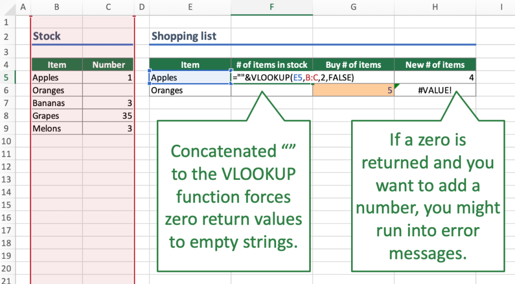
Careful: Return value is interpretated as text.Your VLOOKUP function above is concatenated to an empty string “”. If your return value is 0, the cell will be shown as an empty string. Further calculations might be difficult: For example, if you want to add a number to the return value. Referring directly to the cell, for example =F6+G6 leads to the #VALUE error message as shown above. However, using the SUM function =SUM(F6,G6) still works.
Bottom line: This is an elegant approach, but please test it well if it suits to your Excel model.
Image by Pexels from Pixabay