
Excel for Microsoft 365 Excel 2021 Excel 2019 Excel 2016 Excel 2013 Excel 2010 Excel 2007 More…Less
Unlike other Microsoft Office programs, such as Word, Excel does not provide a button that you can use to highlight all or individual portions of data in a cell.
However, you can mimic highlights on a cell in a worksheet by filling the cells with a highlighting color. For a fast way to mimic a highlight, you can create a custom cell style that you can apply to fill cells with a highlighting color. Then, after you apply that cell style to highlight cells, you can quickly copy the highlighting to other cells by using Format Painter.
If you want to make specific data in a cell stand out, you can display that data in a different font color or format.
Create a cell style to highlight cells
-
Click Home > New Cell Styles.
Notes:
-
If you don’t see Cell Style, click the More
 button next to the cell style gallery.
 -
-
-
In the Style name box, type an appropriate name for the new cell style.
Tip: For example, type Highlight.
-
Click Format.
-
In the Format Cells dialog box, on the Fill tab, select the color that you want to use for the highlight, and then click OK.
-
Click OK to close the Style dialog box.
The new style will be added under Custom in the cell styles box.
-
On the worksheet, select the cells or ranges of cells that you want to highlight. How to select cells?
-
On the Home tab, in the Styles group, click the new custom cell style you created.
Note: Custom cell styles are displayed at the top of the list of cell styles. If you see the cell styles box in the Styles group, and the new cell style is one of the first six cell styles on the list, you can click that cell style directly in the Styles group.
 button next to the cell style gallery.
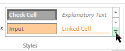
Use Format Painter to apply a highlight to other cells
-
Select a cell that is formatted with the highlight that you want to use.
-
On the Home tab, in the Clipboard group, double-click Format Painter
, and then drag the mouse pointer across as many cells or ranges of cells that you want to highlight. -
When you’re done, click Format Painter again or press ESC to turn it off.
 , and then drag the mouse pointer across as many cells or ranges of cells that you want to highlight.
Display specific data in a different font color or format
-
In a cell, select the data that you want to display in a different color or format.
How to select data in a cell
To select the contents of a cell
Do this
In the cell
Double-click the cell, and then drag across the contents of the cell that you want to select.
In the formula bar
Click the cell, and then drag across the contents of the cell that you want to select in the formula bar.
By using the keyboard
Press F2 to edit the cell, use the arrow keys to position the insertion point, and then press SHIFT+ARROW key to select the contents.
-
On the Home tab, in the Font group, do one of the following:
-
To change the text color, click the arrow next to Font Color
and then, under Theme Colors or Standard Colors, click the color that you want to use. -
To apply the most recently selected text color, click Font Color
. -
To apply a color other than the available theme colors and standard colors, click More Colors, and then define the color that you want to use on the Standard tab or Custom tab of the Colors dialog box.
-
To change the format, click Bold
, Italic , or Underline .Keyboard shortcut You can also press CTRL+B, CTRL+I, or CTRL+U.
-

 and then, under Theme Colors or Standard Colors, click the color that you want to use.
 , Italic
  , or Underline
  .
.Need more help?
Colorize your data for maximum impact
Updated on November 11, 2021
What to Know
- To highlight: Select a cell or group of cells > Home > Cell Styles, and select the color to use as the highlight.
- To highlight text: Select the text > Font Color and choose a color.
- To create a highlight style: Home > Cell Styles > New Cell Style. Enter a name, select Format > Fill, choose color > OK.
This article explains how to highlight in Excel. Additional instructions cover how to create a customized highlight style. Instructions apply to Excel 2019, 2016, and Excel for Microsoft 365.
Why Highlight?
Choosing to highlight cells in Excel can be a great way to make sure data or words stand out or increase readability within a file with a lot of information. You can select both cells and text as a highlight in Excel, and you can also customize the colors to suit your needs. Here’s how to highlight in Excel.
How to Highlight Cells in Excel
Spreadsheet cells are the boxes that contain text within a Microsoft Excel document, though many are also completely empty. Both empty and filled Excel cells can be customized in a variety of different ways, including being given a colored highlight.
-
Open the Microsoft Excel document on your device.
-
Select a cell you want to highlight.
To select a group of cells in Excel, select one, press Shift, then select another. Alternatively, you can select individual cells that are separate from each other by holding down Ctrl while you select them.
-
From the top menu, select Home, followed by Cell Styles.
-
A menu with a variety of cell color options pops up. Hover your mouse cursor over each color to see a live preview of the cell color change in the Excel file.
-
When you find a highlight color that you like, select it to apply the change.
If you change your mind, press Ctrl+Z to undo the cell highlight.
-
Repeat for any other cells that you want to apply a highlight to.
To select all of the cells in a column or row, select the numbers on the side of the document or the letters at the top.
How to Highlight Text in Excel
If you just want to highlight text in Excel instead of the entire cell, you can do that too. Here’s how to highlight in Excel when you just want to change the color of the words in the cell.
-
Open your Microsoft Excel document.
-
Double-click the cell containing text you want to format.
-
Press the left mouse button and drag it across the words you want to colorize to highlight them. A small menu appears.
-
Select the Font Color icon in the small menu to use the default color option or select the arrow next to it to choose a custom color.
You can also use this menu to apply bold or italics style options as you would in Microsoft Word and other text editor programs.
-
Select a text color from the pop-up color palette.
-
The color is applied to the selected text. Select elsewhere in the Excel document to deselect the cell.
How to Create a Microsoft Excel Highlight Style
There are a lot of default cell style options in Microsoft Excel. However, if you don’t like any of the available choices, you can create your own personal style.
-
Open a Microsoft Excel document.
-
Select Home, followed by Cell Styles.
-
Select New Cell Style.
-
Enter a name for the new cell style and then select Format.
-
Select Fill in the Format Cells window.
-
Choose a fill color from the palette. Choose the Alignment, Font or Border tabs to make other changes to the new style and then select OK to save it.
You should now see your custom cell style at the top of the Cell Styles menu.
Thanks for letting us know!
Get the Latest Tech News Delivered Every Day
Subscribe
I have a customer which is using 2010 and having this issue on a daily basis. They are rebooting every night, but when they use the spreadsheet the following day the issue returns, but changes from day to day. The first time they showed the issue to me it was not placing borders around columns D-G when they selected a row, then the next time it’s a different set of columns. I’ve not seen it duplicate the issue for the same set of columns. Nor do the unbordered columns remain the same throughout the day. What’s odd is if the user Alt/Tab’s to a different window, then returns back to the workbook, the selected cells will display the proper borders until the active cell is changed. The workbook contains 2 worksheets, 1 macro, and one pivot table. The largest worksheet only contains approximately 150 row and makes use of 12 columns. When I bring the workbook onto my 2013 system I find no issues. Have searched the internet for a resolution but have had no luck. This thread is the closest I’ve found to others that have had a similar issue. Any ideas, thoughts, or suggestions would be appreciated. Thank you in advance for your communications.
Watch Video – How to Highlight Blank Cells in Excel
When I get a data file from a client/colleague or I download it from a database, I do some basic checks on the data. I do this to make sure there are no missing data points, errors or duplicates that may lead to issues later.
One such check is to find and highlight blank cells in Excel.
There are many reasons that can result in blank cells in a dataset:
- The data is not available.
- Data points accidentally got deleted.
- A formula returns an empty string resulting in a blank cell.
While it’s easy to spot these blank cells in a small dataset, if you have a huge one with hundreds of rows and columns, doing this manually would be highly inefficient and error prone.
In this tutorial, I will show you various ways to find and highlight blank cells in Excel.
Highlight Blank Cells Using Conditional Formatting
Conditional Formatting is a great way to highlight cells based on its value when the given condition is met.
I am going to showcase these examples with a small dataset. However, you can use these same techniques with large datasets as well.
Suppose you have a dataset as shown below:
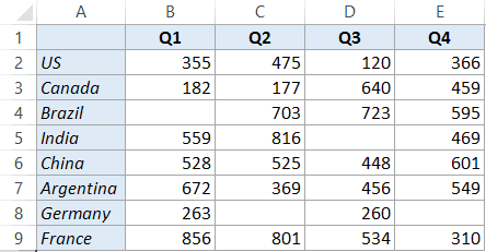
You can see there are blank cells in this dataset.
Here are the steps to highlight blank cells in Excel (using conditional formatting):
This would highlight all the blank cells in the dataset.

Note that conditional formatting is dynamic. This means that if conditional formatting is applied and you delete a data point, that cell would get highlighted automatically.
At the same time, this dynamic behavior comes with an overhead cost. Conditional Formatting is volatile, and if used on large data sets, may slow down your workbook.
Also read: Delete Blank Columns in Excel
Select and Highlight Blank Cells in Excel
If you want to quickly select and highlight cells that are blank, you can use the ‘Go to Special’ technique.
Here are the steps to select and highlight blank cells in Excel:
As mentioned, this method is useful when you want to quickly select all the blank cells and highlight it. You can also use the same steps to select all the blank cells and then fill 0 or NA or any other relevant text in it.
Note that unlike conditional formatting, this method is not dynamic. If you do it once, and then by mistake delete a data point, it will not get highlighted.
Using VBA to Highlight Blank Cells in Excel
You can also use a short VBA code to highlight blank cells in a selected dataset.
This method is more suitable when you need to often find and highlight blank cells in data sets. You can easily use the code below and create an add-in or save it in your personal macro workbook.
Here is the VBA code that will highlight blank cells in the selected dataset:
'Code by Sumit Bansal (https://trumpexcel.com)
Sub HighlightBlankCells()
Dim Dataset As Range
Set Dataset = Selection
Dataset.SpecialCells(xlCellTypeBlanks).Interior.Color = vbRed
End Sub
Here are the steps to put this VBA code in the backend and then use it to highlight blank cells in Excel:
How to Run the VBA code (Macro)?
Once you have copy pasted this macro, there are a couple of ways you can use this macro.
Using the Macro Dialog Box
Here are the steps to run this macro using the Macro dialog box:
- Select the data.
- Go to the Developer tab and click on Macros.

- In the Macro dialog box, select the ‘HighlightBlankCells’ macro and click on Run.


Using the VB Editor
Here are the steps to run this macro using the VB Editor:
- Select the data.
- Go to the Developer tab and click on Visual Basic.

- In the VB Editor, click anywhere within the code.
- Click on the Green triangle button in the toolbar (or hit the F5 key).


As I mentioned, using VBA macro to highlight blank cells is the way to go if you need to do this often.
Apart from the ways shown above to run the macro, you can also create an add-in or save the code in the Personal macro workbook.
This will allow you to access this code from any workbook in your system.
You May Also Like the Following Excel Tutorials:
- How to Find External Links and References in Excel.
- How to Quickly Find and Remove Hyperlinks in Excel.
- Highlight EVERY Other ROW in Excel.
- The Ultimate Guide to Find and Remove Duplicates in Excel.
- Using InStr Function in Excel VBA.
- How to Filter Cells with Bold Font Formatting in Excel.
- How to Compare Two Columns in Excel.
You’re probably thinking that it is no big deal or maybe you’re not, since you’re here reading this guide. But of course, when the task is to highlight blank cells amidst hundreds of rows of a dataset, no one’s laughing now. The Excel gods like your smile and have shined down some easy peasy Excel tricks to sift and highlight blank cells from your data in no time.
In this tutorial, you will learn about «how to highlight blank cells in Excel using Conditional Formatting, filters, the Go To Special feature, and VBA Macro.
Why would anyone need the blank cells highlighted? The blank cells can indicate missing or deleted data or an empty text string resulting from formulas. Blank cells need to be highlighted so they can either be filled or their pertaining data be deleted.
This brings us to an important point. Some cells appear blank but may not really be blank. Find out more below.
 1")
Difference between Blank Cells and Cells that Appear Blank
Blank cells are cells that don’t contain any data. Cells that contain a formula to return empty text (denoted by double-double quotes «» in formulas) or cells that contain a space character may appear blank but are not really blank. The problem with cells that appear blank is that some formulas and features will not treat them as blank cells. For our case, if the cells are not treated as blank, they won’t be highlighted.
The first two methods of highlighting cells in this guide will also work for cells that appear blank while the other two methods will not.
Highlight Blank Cells Using Conditional Formatting
Works for cells that are not blank but appear blank? Yes.
Conditional Formatting is a feature that formats cells according to cell values and as per the provided condition. There are various in-built conditions that you can make use of and there is also the alternative to set a custom condition. We will go with the latter route and specify our own condition to highlight the blank cells from the selected range. Find the complete steps below to highlight blank cells using Conditional Formatting:
- Select the range containing the blank cells.
- In the Home tab, select the Conditional Formatting button in the Styles section. From the menu, hover over Highlight Cells Rules to further expand the menu and select More Rules…
 2")
- The New Formatting Rule dialog box will open.
- Click on the drop-down arrow of the field reading Cell Value and select Blanks from the menu.
 3")
- The dialog box options will lessen to only formatting options. Click on the Format button to set the color fill for the highlighted cells.
 4")
- This will lead to a separate window for choosing the format. In the new Format Cells window, go to the Fill tab and select the color for highlighting the blank cells.
- Click on OK when done.
 5")
- The preview shows the selected color fill.
- Click on the OK button in the New Formatting Rule
 6")
Here are the highlighted blank cells using Conditional Formatting:
 7")
Pros: Being a dynamic feature, Conditional Formatting will automatically adjust with changes to the data. E.g. if you add a value to a blank cell, it would not remain highlighted. Likewise, if you delete a value, the cell will become blank and highlighted.
Cons: While Conditional Formatting is dynamic, it is also volatile; used on large amounts of data, it will slow the file down.
Filter & Highlight Blank Cells
Works for cells that are not blank but appear blank? Yes.
This method of filtering to highlight blank cells works best for tabular data. We will use sorting filters on the dataset. The filter will bunch the blank cells from one column together which can then be selected and highlighted. If more than one column contains blank cells, you can take turns with the columns, filtering and highlighting the blank cells but if you do have more columns, the other methods of highlighting blank cells will be quicker for you.
As mentioned, this method works for cells that appear blank. In the example below, you can see from the formula bar that the cells are not truly blank as the formula is returning an empty text string.
- Select any cell in the dataset and then go to Home tab > Editing section > Sort & Filter button > Filter command or press the Ctrl + Shift + L keys to add columnar filters to the dataset.
 8")
- Here, the filters have been added to the dataset as shown from the little arrows in the headers:
 9")
- Click on the filter of the column containing the blank cells. Uncheck the Select All checkbox and select only the Blanks checkbox.
 10")
- Click on the OK. All the blank cells in the column will group up like so:
 11")
- Select all the blank cells that have been filtered and highlight them with a color of choice from the Fill Color
 12")
- Now it should look something like this:
 13")
- Press the Ctrl + Shift + L keys again to clear the filters. All the data will snap back into place, leaving the blank cells highlighted:
 14")
Select & Highlight Blank Cells
Works for cells that are not blank but appear blank? No.
This method utilizes a mechanical selection of the blank cells so they can be highlighted together. For the mechanical selection, the Go To Special feature will automatically select the blank cells from the dataset. After that, all you have to do is highlight the cells using color fill. Below are the steps to highlight blank cells by selecting them using Go To Special:
- Select the cells with the blanks.
 15")
- Press the Ctrl + G keys or the F5 key to launch the Go To dialog box.
- Select the Special button in the dialog box to open the Go To Special dialog box. (You can also find the Go To Special option in Home tab > Editing group, > Find & Select menu.)
 16")
- Select the Blanks radio button and then the OK
 17")
- From the selection of cells made in the first step, only the blank cells will remain in selection now.
- Use the Fill Color button in the Home tab > Font group to highlight the selected blank cells.
 18")
Be careful not to click anywhere else on the active worksheet; it will change the selection of the cells.
The blank cells will be highlighted/color-filled in the chosen color:
 19")
Highlight Blank Cells Using VBA
Works for cells that are not blank but appear blank? No.
For those with VBA as their right hand, you can also highlight blank cells with a VBA code. VBA allows user-defined functions to automate tasks in Microsoft applications. The task we will assign to VBA is highlighting the blank cells from the selected cells in the color yellow. This task will be assigned via a code that will be fed as a macro using the VB editor. These are the steps to highlight blank cells using VBA:
- Select the cells including the blank cells in the dataset.
- Select the Visual Basic button from the Code section in the Developer tab if you have the tab enabled or you can press the Alt + F11.
- This will open the Visual Basic (VB) editor. Here is what you’ll see when you open the VB editor:
 20")
- Click on the Insert tab and select Module from the list to launch a Module
 21")
- Copy and paste the following code to the Module
Sub HighlightBlankCells()
Dim Dataset As Range
Set Dataset = Selection
Dataset.SpecialCells(xlCellTypeBlanks).Interior.Color = vbYellow
End Sub
This is the code we are using to highlight the blank cells in the dataset from the cells that are in selection. Like the rest of this guide, we have gone with yellow as our choice of color fill but you can edit the code to add your color preference.
 22")
- If you want to run the code right away, press the F5 key and close the VB editor and the cells will be highlighted.
OR
- For running the code later, close the VB editor now. Make sure you select the cells in the dataset before running the code. To run the code, you need to open the Macro. Click on the Macros button in the View tab’s Macro section or press the Alt + F8 keys.
 23")
- Select the relevant Macro and click on the Run command button.
 24")
The Run button will run the code (no surprises there). The blank cells from the selection of cells will be highlighted in the defined color:
 25")
Not that we’re blank on what to do next but this is the end of our tutorial. We quickly outlined and detailed easy methods of highlighting blank cells that you can come back and have a look at when you’re blank on how to highlight so many of them. There will be more teaching from us and here’s your chance to learn everything Excel at point-blank range, so you know you’re not filling all the blanks on your own. Head back when you’re drawing a blank on an Excel predicament! The End (of the tutorial and the saturation of blank puns).
Pointing blank cells in larger data might be a tricky thing to do. You may find it odious, boring, and the most unwanted thing. A blank cell is just a tiny cell in huge crowdedly filled rows and columns of cells. Just a white cell that represents missing data or formula results in an empty string and appears as a black cell.
Importing an Excel file from an external database needs you to check the data so that you can find out missing data points. Though a small datasheet easily allows you to highlight black cells in Excel. On the other side, having a huge data set leads you to find some effective solutions. Manually highlighting hundreds and thousands of rows and columns with blank cells is clearly not possible.
That’s where you need some tricks and tips to highlight blank cells in Excel. Highlighting these empty cells with any color simply makes the task uncomplicated.
How to Highlight Blank Cells in Excel
You must be wondering which method answers perfectly to how to highlight blank cells in Excel. Well, it purely depends upon you as we have come up with more than one method that can help you recognize blank cells. Each method has its significance, so you can try it all randomly.
Here we have tried and proved methods to highlight and color empty cells.
Method # 1: Highlight Blank Cells with Go To Special
With this simple method, you can highlight all blank cells in a suspected range that later on can be filled with any color.
Let’s begin with the process:
- Choose the area or range from where you want to highlight blank cells. Click the upper-left cell and press Ctrl +Shift + End to pick each cell with data. It will make the selection longer till the last used cell.
- Go to the Home tab and choose the “Editing” group. Now, click on Find & Select then Go to Special. Or else you can simply press F5 and click on Special.
- Choose Blanks in the Go To Special dialogue box and press OK.
- It will result in selecting all blank cells in the range.
- As you see all blank cells being selected, fill them with a color to make them prominent.
All done!
Note: Keep in mind that Go To Special method works where your data has truly empty cells. For instance, absolutely blank cells with nothing in them. Also, note that if your data has cells filled with spaces, empty strings, non-printing characters, carriage returns, etc. will not be highlighted because they are not considered as blank.
In either case, you can use another method called Conditional Formatting or VBA macro that we will discuss in this article later.
This is one of the best methods, as you don’t need to repeat the process in any case. Another thing to bear in mind is that any change you make later will not be highlighted or colored. So, you have to keep repeating the method until the last change you make.
Method # 2: Conditional Formatting to Highlight Blank Cells
Here is another greatly effective method to practice:
- At first, you need to choose the data table.
- Now, go to the Home tab and click on Conditional Formatting.
- Next, select the “highlight cell rules” option and click on the “more rules” option.
- From this menu, select the “Blank” option.
- Now, click on the “format” button to start formatting.
- Choose the color you want to use for highlighting from the formatting options.
- Press OK.
Do you know the best part of this method? If your data set has blank cells resulting from a formula, these cells will highlight as well. Moreover, if you are working with a pivot table rather than a normal table, you don’t need to change any step.
Method # 3: Filter Approach
The above two methods work finely with all kinds of data sets. However, if you want to find and highlight blank cells of just rows in a specific column, then you can try this approach.
For this:
- You need to choose all data using the first method’s first step.
- Now, press Ctrl + Shift + L to turn filters on.
- Continue the selection and start filtering the columns you need to represent blank values.
- Now, fill the cells with yellow color.
All Done!
Isn’t it that simple?
Method # 4: Using VBA to Highlight Blank Cells in Excel
Are you familiar with the VBA coding system?
Using a short VBA code can help you highlight empty cells in a selected range. Try this method frequently when you want to find and highlight empty cells in data sets.
Below you will find the VBA code to highlight blank cells in the selected range of the dataset:
Sub Highlight Blank Cells()
Dim Dataset As Range
Set Dataset = Selection
Dataset.Special Cells(xlCellTypeBlanks).Interior.Color = vbRed
End Sub
Now, let’s run this method practically by following some easy steps:
- Go to the Developer tab and click on the Visual Basic option. Or else you can simply press ALT + F11.
- Open the VB editor and right-click on the given sheet names in the Project Explorer. In case, if you don’t find Project Explorer, press Ctrl + R.
- Go to Insert and choose the Module option.
- In the Module code window, you need to copy and paste the VBA code.
Now, close the VB Editor.
To Sum Up
So, these were some of the most efficient methods to practice. You will find each of the above-given methods helpful. It is entirely up to you, which method you choose because each method has its worth. Conditional Formatting is my personal favorite method that I like to use always for highlighting empty cells in all data sets.
If you have come across a method of finding and highlighting blank cells in Excel other than those mentioned above, you are welcome to share with us.
Keep practicing the tricks and enjoy using different methods for the same task.
Unfortunately, this does not work.
[according to «OssieMac»]:
1. Select the cell where you want the color highlighting
2. Select desired text in the formula bar.
3. Set the color as you would for the entire cell
Step 1, fine. Step 2, fine. On Step 3, as soon as I highlight the text in
the formula bar, all cell formatting options are grayed out and inaccessible.
Once that formula bar text is highlighted, the only thing(s) i can do is
edit that text.
I don’t want to change the text color, which by following the suggested
steps only allows me to change the text color.
Am I misinterpreting your suggestion and/or doing something wrong?
OssieMac said:
Hi Ean,
Select the cell where you want the color highlighting and then in the
formula bar at the top select just that part of the text you want to color
and set the color as you would for the entire cell.Regards,
OssieMac
Found this on the net, hopefully it may help:
This article was previously published under Q320531
SYMPTOMS
When you try to change the fill color or the fill pattern in one of the programs listed in the «Applies To» section, the changes that you selected may not be visible. However, you may be able to see the changes in print preview and on a printed page.
Note Print preview and Print still work as expected. The colors are only missing on the screen.
CAUSE
This issue may occur if the Use High Contrast check box is selected.
RESOLUTION
To resolve this issue, follow these steps.
Note Because there are several versions of Microsoft Windows, the following steps may be different on your computer. If they are, see your product documentation to complete these steps. 1. Click Start, click Control Panel, and then click Accessibility Options.
2. Click the Display tab, and then click to clear the Use High Contrast check box.
3. Click OK to close the Accessibility Options dialog box.
MORE INFORMATION
High contrast color schemes make the screen easier to view by heightening screen contrast with alternative color combinations. Some of these schemes also change the font sizes for easier reading.
Was this post helpful?
thumb_up
thumb_down